A Jones matrix formalism for simulating three-dimensional polarized light imaging of brain tissue

Abstract

The neuroimaging technique three-dimensional polarized light imaging (3D-PLI) provides a high-resolution reconstruction of nerve fibres in human post-mortem brains. The orientations of the fibres are derived from birefringence measurements of histological brain sections assuming that the nerve fibres—consisting of an axon and a surrounding myelin sheath—are uniaxial birefringent and that the measured optic axis is oriented in the direction of the nerve fibres (macroscopic model). Although experimental studies support this assumption, the molecular structure of the myelin sheath suggests that the birefringence of a nerve fibre can be described more precisely by multiple optic axes oriented radially around the fibre axis (microscopic model). In this paper, we compare the use of the macroscopic and the microscopic model for simulating 3D-PLI by means of the Jones matrix formalism. The simulations show that the macroscopic model ensures a reliable estimation of the fibre orientations as long as the polarimeter does not resolve structures smaller than the diameter of single fibres. In the case of fibre bundles, polarimeters with even higher resolutions can be used without losing reliability. When taking the myelin density into account, the derived fibre orientations are considerably improved.

1. Introduction

Unravelling the architecture and connectivity of nerve fibres in the human brain is one of the greatest challenges in neuroscience. Over the past years, several methods have been developed to reconstruct the human connectome [1–3]. The neuroimaging technique three-dimensional polarized light imaging (3D-PLI) has been employed to reconstruct the three-dimensional architecture of nerve fibres in human post-mortem brains with a resolution of a few micrometres [4,5]. 3D-PLI enables the investigation of the pathways of long-range fibre bundles as well as single fibres and thus serves as a bridging technology between the macroscopic and the microscopic scale.

The spatial orientations of the nerve fibres are derived by transmitting polarized light through histological brain sections in a polarimeter and measuring their birefringence. To relate the measured signal to the fibre orientation, an effective model of birefringence is used which assumes that the fibre density is constant over the whole brain section [4] and that the measured optic axis indicates the predominant fibre orientation [5,6]. This assumption is based on various experimental studies on white matter which show that the average birefringence of parallel nerve fibres is negatively uniaxial and that the measured optic axis is oriented along the length of the fibres [7–10].

The majority of nerve fibres in the brain consist of an axon and a surrounding myelin sheath. The cytoplasm of the axon contains tubular polymers (microtubules) and neurofilaments running along the length of the axon [11,12]. The myelin sheath is formed by oligodendrocytes (glial cells) which are spirally wrapped around the axon. The cell membranes are bimolecular layers consisting of lipid molecules and membrane proteins. The membrane proteins are embedded in the bilayer or attached to the membrane surface [13–15], whereas the lipid molecules are oriented radially to the fibre axis [15–17]. The cell organelles of the axon and the protein framework of the myelin sheath lead to a weak positive birefringence with respect to the longitudinal fibre axis [7,8,10,17–20]. The anisotropic structure of the lipid molecules causes a positive birefringence with respect to the radial fibre axis [7,8,15,18,21].

The effective model of uniaxial negative birefringence that is currently used in 3D-PLI seems reasonable for sufficiently low optical resolutions. However, it might no longer be valid if the anisotropic molecular structure of the nerve fibres is resolved. In this paper, we investigated the limitations of the effective model in terms of the optical resolution of the polarimeter using numerical simulations. The simulations were performed with a modified version of SimPLI [6], a simulation method that models the birefringence of the fibres with the Jones matrix calculus and allows data to be generated from synthetic fibre constellations that is comparable to experimental data. In order to study and understand the most dominant effects that generate the birefringence signals in 3D-PLI, the anisotropic molecular structure of the nerve fibres was described by a simplified birefringence model with radial optic axes (microscopic model) and the effective model of uniaxial negative birefringence by a birefringence model with axial optic axes (macroscopic model). To investigate the limitations of the effective model, the transition between the microscopic and the macroscopic model was investigated depending on the optical resolution of the imaging system.

2. Three-dimensional polarized light imaging

The neuroimaging technique 3D-PLI determines the orientation of nerve fibres in post-mortem brains at the micrometre scale. The principles of 3D-PLI have been explained in detail by Larsen et al. [22] and Axer et al. [4,5]. This section describes the measurement and data analysis procedures that are relevant for this study.

2.1. Measurement

To determine the orientation of the nerve fibres, a post-mortem brain—obtained from a body donor in accordance with ethical requirements—is fixed in buffered formaldehyde for several months, frozen and cut with a cryotome into histological sections of 70 µm, which are measured with a polarimeter. For the 3D-PLI measurement, two state-of-the-art polarimeters with different optical resolutions and sensitivities are employed: the large-area polarimeter (LAP) has a pixel size of 64 µm and is mainly used for single-shot images of whole human brain sections. The polarizing microscope (PM) has a pixel size of 1.33 µm (i.e. down to small axonal diameters), which enables complex fibre constellations to be disentangled.

The LAP contains a pair of crossed linear polarizers and a quarter-wave retarder (with its fast axis adjusted at an angle of −45° with respect to the transmission axis of the first linear polarizer) (figure 1a). The employed light source emits incoherent, non-polarized, diffusive light with a peak wavelength of 525 nm. During the measurement, the polarizers and the quarter-wave retarder are rotated simultaneously around the stationary tissue sample. For each rotation angle ρ = 0°, 10°, … , 170°, the transmitted light intensity is recorded by a CCD camera so that a series of 18 images is acquired.

Figure 1.

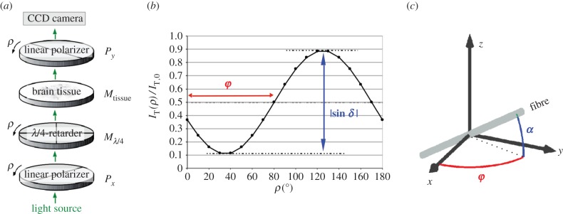
(a) Measurement set-up of 3D-PLI (for the LAP): the brain tissue is placed between a pair of crossed linear polarizers and a quarter-wave retarder, which are rotated simultaneously by 18 discrete rotation angles ρ. The transmitted light intensity is calculated with the Jones calculus, in which each optical element is represented by a Jones matrix (symbols on the right). (b) The normalized transmitted light intensity describes a sinusoidal curve for each image pixel. The phase φ corresponds to the local fibre direction angle and the peak-to-peak amplitude to the local fibre inclination angle. (c) The three-dimensional orientation of a fibre is defined by the direction angle φ and the inclination angle α. (Online version in colour.)

The imaging principle works as follows: the quarter-wave retarder transforms the linearly polarized light from the first polarizer into circularly polarized light. The birefringent brain tissue induces an additional phase shift so that the outgoing light is elliptically polarized. The fraction of light that then passes the second linear polarizer depends on the local orientation of the optic axis of the birefringent tissue, which is assumed to coincide with the local fibre orientation.

The polarimetric set-up of the PM is slightly different to the set-up of the LAP (the order of the optical elements is reversed and only the first linear polarizer is rotatable). However, the imaging principle and the signal analysis are similar [4] so that the following considerations are only described for the LAP.

2.2. Signal analysis

The measured light intensity of an individual pixel describes a sinusoidal curve across the acquired image series, which depends on the orientation of the fibres within this pixel (figure 1b). A physical description of the measured light intensity profile can be derived with the Jones matrix calculus [23,24], assuming that the light is coherent and completely polarized and that the optical elements are linear. For simplicity, the derivation is shown for a single pixel at a certain rotation angle ρ.

In the Jones matrix calculus, all optical elements in the polarimeter are represented by Jones matrices (cf. figure 1a). The Jones matrices of the crossed linear polarizers are given by [25]

2.1

The Jones matrix of a wave retarder that is rotated by an angle ψ in counterclockwise direction and induces along the fast axis a phase shift δ between the two orthogonal components of the light wave is given by [25]

2.2

In the experimental set-up, the fast axis of the quarter-wave retarder is rotated by −45° with respect to the axis of the first linear polarizer. Thus, the quarter-wave retarder can be described by the Jones matrix of a rotated wave retarder as given in equation (2.2) with a rotation angle of ψ = −45° and a phase shift of δ = 90°:

2.3

Under the assumption that the birefringence of the brain tissue can locally be described as negatively uniaxial with the optic axis indicating the predominant fibre direction (effective model), the brain tissue can locally be represented by a wave retarder that introduces a phase shift δ along the fast axis (fibre axis). During the measurement, the two polarizers and the quarter-wave retarder are rotated simultaneously around the specimen stage in counterclockwise direction by a rotation angle ρ. For simplicity, the equivalent case is considered in which the brain tissue is rotated by an angle (−ρ) in counterclockwise direction while the other optical elements are fixed. Thus, the brain tissue can be described by the Jones matrix of a rotated wave retarder as given in equation (2.2) with phase shift δ and rotation angle ψ = φ − ρ, where φ denotes the in-plane orientation of the optic axis:

2.4

When light with an electric field vector E₀ passes through the 3D-PLI set-up, the resulting output beam with electric field vector E_T can be described by multiplication of the associated Jones matrices. As the Jones matrix calculus cannot be used to describe the non-polarized light emitted by the employed light source, the Jones vector is used to describe the horizontally polarized light after the first linear polarizer (cf. figure 1a):

2.5

Using , the transmitted light intensity is calculated, yielding a sinusoidal intensity profile (figure 1b):

2.6

where corresponds to the transmitted light intensity averaged over all rotation angles (here referred to as transmittance) and to the peak-to-peak amplitude of the normalized sinusoidal intensity profile (here referred to as retardation). The phase shift δ is given by (appendix A)

2.7

where λ is the wavelength of the incident light, t the thickness of the brain section, Δn the local birefringence of the sample and α the local out-of-plane inclination angle of the fibre. Thus, the intensity profile in equation (2.6) is a direct measure of the spatial fibre orientation defined by the direction angle φ and the inclination angle α (figure 1c).

In order to compute transmittance, direction and retardation, the intensity profile is fitted by means of a discrete harmonic Fourier analysis [4,26]. The inclination angle α is calculated from the measured retardation by rearranging equation (2.7). The direction and inclination angles are combined to a unit vector indicating the local fibre orientation in three dimensions. Putting all unit vectors of several adjacent brain sections together, a three-dimensional volume of vectors is created and the fibre tracts are reconstructed with streamline algorithms.

3. Simulation of three-dimensional polarized light imaging using the Jones matrix formalism

3.1. Simulation model

3D-PLI derives the nerve fibre orientations based on the fact that the average birefringence of parallel fibres is negatively uniaxial [7–10] and assuming that the orientation of the measured optic axis corresponds to the local fibre orientation. To investigate the limitations of this effective birefringence model, a straight single fibre and a hexagonal bundle of straight parallel fibres were simulated and the birefringence of the fibres was modelled according to a microscopic and a macroscopic model for different optical resolutions of the simulated imaging system.

3.1.1. Microscopic model

The microscopic model of birefringence considers the anisotropic molecular structure of a single nerve fibre. To investigate and understand the predominant effects generating the birefringence signals in 3D-PLI, a simplified model of birefringence was chosen for the simulations. As stated in §1, the average birefringence of parallel nerve fibres is negative with respect to the longitudinal fibre axis. Therefore, the positive birefringence of the axon and the myelin proteins is weak as compared to the birefringence effects of the myelin lipids [8,9,18,20,21]. Since the exact contribution of the different birefringence effects to the overall birefringence is unknown, the birefringence effects of the nerve fibres were modelled by considering only the anisotropic radial structure of the myelin sheaths: the fibres were simulated as hollow tubes (representing the myelin sheaths) with positive birefringence and radial optic axes (cf. figure 2b(ii)). The axons were considered to be non-birefringent.

Figure 2.

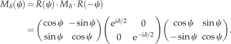
Simulation method: (a) generation of synthetic nerve fibres in a three-dimensional volume. (b) Generation of a three-dimensional vector field according to the macroscopic model (i, axial optic axes) and the microscopic model (ii, radial optic axes). (c) Generation of a synthetic 3D-PLI image series (illustrated for a large fibre in the microscopic model): the simulation volume is discretized into small volume elements (voxels). Each myelin voxel (grey) is represented by the Jones matrix of an optical retarder (M_j) whose axis is oriented in the direction of the optic axes (arrows). The polarizing filters of the 3D-PLI set-up (figure 1a) are also represented by Jones matrices. For each rotation angle of the polarimeter, all Jones matrices along the optical path (highlighted column) are multiplied. (Online version in colour.)

3.1.2. Macroscopic model

To compare the simulation results of the microscopic model with the effective model of uniaxial negative birefringence, a macroscopic model of birefringence was defined. According to the assumptions made in the effective model, a single nerve fibre was simulated as negatively birefringent with axial optic axes oriented along the length of the fibre (cf. figure 2b(i)). Dohmen et al. [6] used this simulation model to investigate the effect of crossing fibre constellations. As this study concentrates on straight parallel fibres, the macroscopic model only serves as a reference for the effective model to verify the simulations of the microscopic model. To ensure a better comparison with the microscopic model, the fibres were simulated as hollow tubes (and not as solid cylinders as in [6]).

3.2. Simulation method

The basic idea of the simulation method is to model the birefringent myelin sheaths as series of linear optical retarder elements which are represented by Jones matrices. By defining the direction of the optic axes (radial/axial), both the microscopic and the macroscopic model can be simulated. The simulation approach is based on the simulation tool SimPLI developed by Dohmen et al. [6]. For this study, the simulation tool was extended by the microscopic model and modified such that various fibre configurations with individual orientations, radii and myelin sheath thickness can be realized.

The simulation tool is based on several assumptions and simplifications: first of all, the use of the Jones matrix calculus requires linear optical elements and perfect polarizers (i.e. the outgoing light is assumed to be completely polarized). Another assumption is that the incident light can be described by parallel rays of light with straight optical pathways, i.e. the light is assumed to be non-diffusive and refraction, diffraction and scattering are neglected. For this study, a parallel and straight beam of light seems a reasonable approximation for the LAP because the imaging system has a small numerical aperture (the acceptance angle of the objective lens is less than 1°) so that the camera only captures light rays that are almost parallel to each other.

The simulation consists of several steps:

• (1) Generation of synthetic nerve fibres in a three-dimensional volume. The nerve fibres are modelled as hollow tubes representing the myelin sheaths (figure 2a). In order to approximate the geometry of the fibres, the simulation volume is discretized into small cubic volume elements (called voxels), as indicated schematically by the grid in figure 2c.

• (2) Generation of a three-dimensional vector field. For sufficiently small voxel sizes, the birefringence of the myelin sheaths can approximately be described by assigning each myelin voxel j a unit vector that indicates the direction of the optic axis (φ_j, α_j) within the myelin sheath. In the macroscopic model, the vectors are oriented parallel to the fibre axis. In the microscopic model, the vectors are oriented radially to the fibre axis (figure 2b).

• (3) Generation of a synthetic 3D-PLI image series. In order to model the birefringence effect of the myelin sheaths, each myelin voxel is represented by the Jones matrix of a rotated wave retarder. The retarder axis is aligned with the optic axis within the myelin voxel (figure 2c). The synthetic 3D-PLI image series is calculated analogously to the derivation of the sinusoidal intensity profile as given in equation (2.5), with M_tissue being replaced by the product of N matrices representing the myelin voxels along the optical path:

  3.1

  The matrix is the Jones matrix of a rotated wave retarder as given in equation (2.2) and represents the jth myelin voxel. The rotation angle depends on the in-plane direction angle φ_j of the optic axis and the phase shift δ_j on the out-of-plane inclination angle α_j. The Jones matrices of the linear polarizers and the quarter-wave retarder are given by equations (2.1) and (2.3). For each rotation angle of the polarimeter (ρ = 0°, 10°, … , 170°), all Jones matrices along the optical path are multiplied (figure 2c), yielding a series of 18 synthetic 3D-PLI images with a sinusoidal intensity profile for each image pixel.

3.3. Simulation parameters

The choice of the simulation parameters was inspired by real experimental conditions. According to typical dimensions of large nerve fibres in human white matter [16,27–29], the diameter and the myelin sheath thickness of the simulated nerve fibres were chosen to be 15 µm and 2.5 µm, respectively (figure 3a). The fibres were generated in a simulation volume with dimensions x × y × z = 64 × 64 × 70 µm³, corresponding to the pixel size of the LAP and the thickness of the brain section. The simulation volume was discretized into cubic voxels with a side length of Δx_sim. In a preliminary study (see later, §4.1), the optimal voxel size was determined to be Δx_sim = 0.1 µm, which was used for all following simulations. Note that the dimensions are given in micrometres to meet the experimental conditions. As only relative length scales matter for the qualitative simulation results, the units could be chosen arbitrarily.

Figure 3.

(a) Dimensions of the simulated fibre (cross-sectional view). (b) Simulation model for comparison with the analytical solution: a horizontal fibre is simulated with outer radius r₁ = 7.5 µm, inner radius r₂ = 5 µm, and radial optic axes. The light is incident perpendicular to the fibre axis at distance r₀. The electric field vector of the ordinary wave (E₀) is oriented parallel to the longitudinal axis of the fibre. The electric field vector of the extraordinary wave (E_e) is oriented perpendicular to the fibre axis. (Online version in colour.)

Since measuring the birefringence of the micrometre-thick brain sections is impossible with the employed set-ups and literature values are not given for the currently used preparation technique, an upper limit for the birefringence of the myelin sheaths Δn was estimated: under the assumption that a brain section that is completely filled with a homogeneous birefringent material with in-plane optic axis (α = 0°) induces a maximum possible retardation the upper limit of the birefringence was calculated by rearranging equation (2.7): Note that the choice of Δn only changes the overall magnitude of the retardation and does not affect the simulation results qualitatively. In the macroscopic (microscopic) model, the myelin voxels were simulated with axial (radial) optic axes and negative (positive) birefringence with respect to the optic axes.

The wavelength of the incident light was chosen to correspond to the peak wavelength of the LAP (λ = 525 nm). To study only the birefringence effect of the nerve fibres, the fibres were simulated without any absorption.

3.4. Simulation of the optical resolution

To investigate the effect of different optical resolutions on the measured 3D-PLI signal, the synthetic 3D-PLI image series were downsampled using the open-source image processing programme Fiji [30]: to account for the limited optical resolution of the polarimeter, the image series were first convoluted with a two-dimensional Gaussian filter with a standard deviation σ. Then, the effect of the spatial discretization of the CCD chip was modelled by resampling the resulting images with a sampling factor f_s (average when downsizing). To determine realistic parameters for σ and f_s, the imaging properties of the LAP were considered as a point of reference (appendix B).

Based on these considerations, the synthetic 3D-PLI image series were downsampled with different parameter sets (table 1), yielding images with different pixel sizes Δx. The pixel size of the downsampled images was chosen such that a multiple of the pixel size corresponds to the side length of the simulation volume (Δx = 64 µm/n, with n = 4, 8, 16, 32). The standard deviation was calculated as a linear function of the pixel size (σ = 0.714 Δx, appendix B) and the sampling factor was calculated by dividing the pixel size of the high-resolution image series by the pixel size of the downsampled image . In the following, the optical resolution of the imaging system will be given in terms of the pixel size, which defines the set of downsampling parameters (σ and f_s) in table 1. Note that the simulation results will not change qualitatively as long as the ratio between the fibre dimensions and the downsampling parameters remains the same.

Table 1.

Downsampling parameters (selected values): to obtain an image with pixel size Δx, a two-dimensional Gaussian filter with standard deviation σ = 0.714 Δx and resampling with sampling factor f_s = 0.1 µm/Δx are applied to the image.

Δx (μm)	σ (μm)	fs
2	1.43	1/20
4	2.86	1/40
8	5.71	1/80
16	11.43	1/160

3.5. Calculation of the retardation curve

The determination of the inclination angle α is challenging for 3D-PLI because the peak-to-peak amplitude of the measured intensity profile is highly sensitive to noise and—among others—influenced by the density of myelinated nerve fibres (see below).

In the standard 3D-PLI analysis, the inclination angle is calculated from the measured intensity profile assuming that the brain tissue can locally be described by the effective model of uniaxial negative birefringence. In order to investigate whether the effective model can be used to extract the correct fibre inclinations, the retardation computed from equation (2.7) was compared to the retardation values derived from simulations using the macroscopic and the microscopic model (see §3.1). For that purpose, the retardation images were calculated for different fibre inclinations and different optical resolutions, respectively. For a better comparison between the retardation values of the single fibre and the fibre bundle, only the pixel in the centre of each (downsampled) retardation image was considered for evaluation. If pixels at other locations had been chosen, the retardation values of the single fibre would have been influenced by boundary effects that do not exist for the fibre bundle or real brain tissue which are completely filled with fibres. The retardation values from the centre of each downsampled retardation image were plotted against the corresponding inclination angle, yielding a retardation curve for each downsampling step. The retardation curves were compared to the normalized retardation curve of the effective model (cf. equation (2.7)), in the following referred to as the theoretical curve: .

To be able to compare different retardation curves, the retardation was normalized for each curve with the maximum retardation value, respectively:

3.2

As only birefringent material (mainly myelin) is responsible for the phase shift in equation (2.7), t describes not the thickness of the whole brain section but rather the local myelin thickness t_m, i.e. the combined thickness of myelin sheaths along the optical path. Due to the inhomogeneity of brain tissue, the local myelin density of a brain section is less than 100% i.e. the maximum possible retardation is . If the inclination is calculated under the assumption that the maximum possible retardation equals 1, the inclination angle will be overestimated. In order to obtain a more precise estimation of the inclination angle, a so-called myelin density correction was applied to the downsampled retardation images.

In the case of the macroscopic model, in which the optic axes within one fibre have the same orientations, δ scales linearly with t_m. In the case of the microscopic model, in which the optic axes within one fibre have different inclination angles, the upper limit of δ scales linearly with t_m as long as the optic axes of neighbouring myelin voxels have similar orientations (appendix C). Thus, the dependence on the myelin density can be eliminated to the greatest possible extent by multiplying the phase shift δ with a correction factor (t/t_m):

3.3

In order to apply the myelin density correction to the downsampled retardation images, t_m was replaced by the combined thickness of myelin voxels along the optical path (after applying the Gaussian filter and resampling). The resulting retardation images were normalized according to equation (3.2), yielding .

4. Simulation results

4.1. Comparison of analytical and numerical solution

To estimate the accuracy of the simulation results for the microscopic model, a single fibre with radial optic axes and perpendicularly incident light (figure 3b) was generated for different voxel sizes (Δx_sim) and the numerically computed phase difference between extraordinary and ordinary wave (ΔΦ_num) was compared to the analytical solution (ΔΦ_ana).

Assuming that reflection and refraction effects can be neglected so that the associated extraordinary and ordinary waves follow the same pathway, Bear & Schmidt [18] derived an analytical expression for the phase difference:

4.1

where Γ is the optical path length difference between the extraordinary and ordinary waves, r₁ the radius of the whole nerve fibre (outer cylinder), r₂ the radius of the non-birefringent axon (inner cylinder) and r₀ the distance at which the light is incident perpendicular to the fibre axis (figure 3b).

In order to compute ΔΦ_num, the propagation of the ordinary and extraordinary waves was simulated separately: in the case of the ordinary wave, the light is polarized parallel to the longitudinal axis of the fibre. In the case of the extraordinary wave, the light is polarized perpendicular to the longitudinal axis of the fibre (figure 3b). The phase for both the ordinary wave (Φ_o) and the extraordinary wave (Φ_e) was calculated from the corresponding electric field vector E_T in equation (3.1):

4.2

The numerically computed phase difference ΔΦ_num = Φ_e − Φ_o was evaluated at various distances 0 < r₀ < 5 µm away from the centre of the fibre and compared to the analytical solution given in equation (4.1), with r₁ = 7.5 µm, r₂ = 5 µm, λ = 525 nm and Δn = 0.001875 (cf. §3.3). In order to study the impact of the spatial discretization on the accuracy of the numerical solution, the simulation was performed for various voxel sizes 1.50 µm > Δx_sim > 0.06 µm. As a measure of consistency between the numerical and the analytical solution, the relative phase difference was calculated: (ΔΦ_ana − ΔΦ_num)/ΔΦ_ana.

Figure 4a,b shows the relative phase difference plotted against r₀ for various voxel sizes Δx_sim. As can be seen, the numerical solution fluctuates around the analytical solution for voxel sizes of 0.5 µm and less. With smaller voxel sizes, the numerical solution approaches the analytical solution (indicated by the dashed black line). This behaviour is especially evident when considering the mean of the absolute relative phase difference for each voxel size (figure 4c): for a voxel size of Δx_sim = 1.5 µm (corresponding to one-tenth of the fibre diameter), the mean absolute relative phase difference is about 12%. For Δx_sim = 0.5 µm, it is about 6% and for Δx_sim = 0.06 µm, it is only 0.8%. This demonstrates that the simulation tool produces correct results.

Figure 4.

(a,b) Relative difference between analytically and numerically calculated phase difference (ΔΦ_ana and ΔΦ_num) for various voxel sizes Δx_sim, evaluated at different distances r₀ away from the centre of the fibre. For reasons of clarity, the results are presented in two diagrams: (a) Δx_sim = 1.50−0.21 µm, (b) Δx_sim = 0.17−0.06 µm. The dashed black lines indicate the point at which the numerical values match the analytical solution. (c) Mean absolute relative phase difference plotted against the voxel size Δx_sim. The arrow indicates the voxel size (Δx_sim = 0.1 µm) that is chosen for the fibre simulations. (Online version in colour.)

As a good compromise between computation time and accuracy, all following fibre simulations were performed with a voxel size of Δx_sim = 0.1 µm (corresponding to 1/150 of the fibre diameter). For this voxel size, the relative phase difference is no more than 4% (figure 4b) and the mean relative phase difference is about 1.3% (figure 4c).

4.2. Simulation of a single fibre

In a preliminary study, the limitations of the effective model of uniaxial negative birefringence were first studied for a straight single fibre. The fibre was simulated according to both the macroscopic and the microscopic models with different inclination angles (α = 0°, 10°, … , 90°) and different optical resolutions. The dimensions of the fibre and the other simulation parameters were chosen as described in §3.3. The retardation curves were calculated from the downsampled retardation images (without/with myelin density correction) and normalized as described in §3.5. An example of downsampled and corrected retardation images can be found in appendix D.

Figure 5 shows the dimensions of the simulated single fibre and the corresponding retardation curves (continuous lines) for both simulation models and different optical resolutions (according to table 1). The theoretical retardation curve of the effective model is indicated by a dashed black line. In the case of the macroscopic model, the uncorrected retardation curves (figure 5a) are already very similar to the theoretical curve for all investigated optical resolutions. After the myelin density correction (figure 5c), all retardation curves match the theoretical curve exactly, independently of the optical resolution. In the case of the microscopic model (figure 5b,d), the retardation curves for a pixel size much smaller than the fibre diameter (Δx < 2 µm) are inverted as compared to the theoretical curve for α < 90°, i.e. the microscopic and the macroscopic model yield totally different results. For intermediate pixel sizes (2 µm ≤ Δx ≤ 8 µm), the retardation curves are non-monotonic, i.e. the assignment of the inclination angle is ambiguous. Finally, for pixel sizes larger than the fibre diameter (Δx = 16 µm), the uncorrected retardation curve (figure 5b) is similar to the theoretical curve. After the myelin density correction (figure 5d), the retardation curve matches the theoretical curve almost exactly.

Figure 5.

(a–d) Normalized retardation curves of a straight single fibre simulated according to the macroscopic model (a,c) and the microscopic model (b,d) for different optical resolutions. Graphs (a,b) show the uncorrected retardation curves, graphs (c,d) show the retardation curves after the myelin density correction. For reasons of clarity, only selected graphs are shown. The legend indicates the pixel sizes of the retardation images from which the retardation curves have been calculated. The pixel size Δx of the downsampled retardation images determines the parameters used for simulating the optical resolution (table 1). For better comparison, Δx is also given in terms of the fibre diameter (d = 15 µm). (e) Dimensions of the simulated single fibre. (Online version in colour.)

4.3. Simulation of a fibre bundle

In brain tissue, nerve fibres are usually organized in hexagonal close-packed fibre bundles [13]. In order to investigate the effect of fibre bundles on the 3D-PLI signal, a hexagonal bundle of straight parallel fibres with an inter-fibre spacing of 1 μm was simulated (figure 6e). In order to obtain comparable results, the same dimensions and simulation parameters were chosen as for the single fibre.

Figure 6.

(a–d) Normalized retardation curves of a hexagonal fibre bundle simulated according to the macroscopic model (a,c) and the microscopic model (b,d) for different optical resolutions. Graphs (a,b) show the uncorrected retardation curves, graphs (c,d) show the retardation curves after the myelin density correction. For reasons of clarity, only selected graphs are shown. The legend indicates the pixel sizes of the retardation images from which the retardation curves have been calculated. The pixel size Δx of the downsampled retardation images determines the parameters used for simulating the optical resolution (table 1). For better comparison, Δx is also given in terms of the fibre diameter (d = 15 µm). (e) Dimensions of the simulated fibre bundle. (Online version in colour.)

Figure 6 shows the normalized retardation curves for both simulation models and different optical resolutions (according to table 1). The (downsampled) retardation images that were used to compute the corrected retardation curves of the microscopic model are shown in appendix D.

In the case of the macroscopic model, the uncorrected retardation curves (figure 6a) are very similar to the theoretical retardation curve of the effective model (dashed black line) for all investigated optical resolutions. As compared to the retardation curves of the single fibre (figure 5a), the retardation curves of the fibre bundle are closer to the theoretical curve. After the myelin density correction (figure 6c), the curves are almost identical. In the case of the microscopic model, the uncorrected retardation curves (figure 6b) are also closer to the theoretical curve as compared to the uncorrected retardation curves of the single fibre (figure 5b). The myelin density correction (figure 6d) makes only a small difference, especially for low optical resolutions. For the simulated fibre bundle, the transition between the microscopic and the macroscopic model already occurs for pixel sizes larger than the fibre radius (Δx ≥ 8 µm).

5. Discussion

In 3D-PLI, the fibre orientations are derived under the assumption that the brain tissue can (locally) be described as a homogeneous and uniaxial birefringent material with the optic axis indicating the predominant fibre direction. Furthermore, the density of myelinated fibres is assumed to be the same for the whole brain section. In this paper, the limitations of this effective birefringence model have been studied for the first time. For that purpose, a single fibre and a hexagonal fibre bundle (with diameters d) were simulated based on the Jones matrix calculus, employing a microscopic and a macroscopic model of birefringence and different optical resolutions (defined by the pixel size Δx as given in table 1).

The transition between the two models is apparent when analysing the retardation curves: for high optical resolutions the radial optic axes of the microscopic model are resolved. In this case, the optic axes are oriented perpendicular to the longitudinal fibre axis so that the retardation curves are inverted as compared to the macroscopic model and fibres with high inclination angles are interpreted as flat fibres. The zero retardation value for α = 90° is an artefact arising from the fact that the retardation is evaluated at the centre of the retardation image which—in the case of vertical fibres—contains no myelin (cf. figure 8, upper right corner). For intermediate optical resolutions (Δx < d), there is a transition zone between the microscopic and the macroscopic model so that an unambiguous assignment between retardation and inclination is not possible. For sufficiently low optical resolutions (single fibre: Δx > d; fibre bundle: Δx > d/2), the microscopic and the macroscopic model yield similar results (figures 5d and 6d) so that the effective model of uniaxial negative birefringence can be used to compute the fibre inclinations.

Thus, for the simulated fibre bundle (consisting of five fibre layers with d = 15 µm), the effective model can be used to interpret LAP measurements (Δx_LAP = 64 µm > d/2), but not to interpret PM measurements (Δx_PM = 1.33 µm < d/2). However, the diameters of the simulated fibres represent an upper estimate of typical fibre diameters in the human brain. The diameters of myelinated nerve fibres range from 0.3 to 15 µm [16,27–29] and the majority of the fibres (e.g. 80% in the corpus callosum [27]) have diameters of 1 µm or below so that the condition Δx_PM > d/2 is still fulfilled. In addition, fibre diameters much smaller than 15 µm implicate that the measured brain section (with thickness 70 µm) contains much more fibre layers than the simulated fibre bundle. A comparison between the simulated single fibre and the fibre bundle suggests that the more fibre layers located along the optical path, the smaller the minimum pixel size for which the effective model is still valid. To verify this hypothesis, the limitations of the effective model should also be studied in terms of the number of fibre layers along the optical path. However, a larger number of fibre layers also increases the probability that fibres with different spatial orientations are measured within the same volume, which poses a major challenge for 3D-PLI [6]. In future studies, the limitations of the effective model should therefore also be investigated for non-parallel fibre structures.

The simulations have shown that—in regions with parallel fibre structures—the effective model of uniaxial negative birefringence is valid for the employed optical set-ups. For imaging systems with very high optical resolutions, the effective model needs to be reconsidered. Even if the optical resolution is too high to extract the correct fibre inclinations, 3D-PLI remains a valuable neuroimaging technique as the image contrasts of transmittance and retardation still provide detailed structural information on the two-dimensional nerve fibre architecture in large histological brain sections.

The effective model that is currently used for the data analysis in 3D-PLI does not only assume parallel fibre structures, but also a uniform myelin density. The simulations have shown that the retardation signal is considerably influenced by the myelin density, which impairs the reconstructed fibre orientations. It could be demonstrated that the estimation of the fibre inclination is considerably improved by the myelin density correction which incorporates the local myelin thickness of the examined tissue into the calculation of the inclination angle. While the correction has a large effect on the retardation curves of the single fibre, the effect is smaller for the fibre bundle which is much more homogeneous than the single fibre. Thus, the myelin density correction is especially useful for regions with an inhomogeneous density of myelinated nerve fibres (e.g. for transition zones between white and grey matter). In the case of the microscopic model, the correction does not work as well as for the macroscopic model because the retardation also depends on the direction of the radially oriented optic axes in the myelin sheath, but it is still a considerable improvement. In order to incorporate the myelin density correction into the 3D-PLI signal analysis, the local myelin thickness t_m of the sample needs to be determined. The intensity values of the transmittance image seem to be a good measure of the local myelin thickness in brain tissue [5].

The purpose of this study was to explore and understand the most dominant effects that generate the birefringence signals in 3D-PLI. To fully understand the physical processes behind 3D-PLI and to improve the interpretation of the reconstructed fibre orientations, a direct comparison between simulation and experiment is required. The long-term aim should be to develop a simulation tool of 3D-PLI that considers all relevant effects needed for reproducing the experimental results. To this end, the simulation model should be extended step by step and the relevant effects should be identified.

Although the simulations show that the simplified microscopic model can already be used to explain the effective negative birefringence of parallel nerve fibres, future studies should include the positive birefringence of the axon and investigate how this modification changes the transition between the microscopic and the macroscopic model.

So far, only straight and parallel fibres have been investigated. To provide more realistic fibre models, the fibres should be simulated with varying fibre diameters, myelin sheath thickness and spatial orientations. As fibres with different spatial orientations pose a major challenge for 3D-PLI [6], future studies should focus on investigating inhomogeneous, non-parallel fibre structures. To enable a direct comparison with the experiment, the simulated fibre configurations should be based on experimentally determined fibre structures.

In addition to a more realistic fibre model, the propagation of light should also be simulated more realistically. In this study, the incident light was described by a parallel beam of light. However, in the experiment, the employed light source emits diffusive light, i.e. the sample is illuminated by light with slightly different angles of incidence. As the measured birefringence signals depend on the angle between the light wave and the nerve fibres, a non-zero angle of incidence changes the retardation curves. For the LAP, which has a small numerical aperture, the effect can presumably be neglected. However, for systems with higher optical resolutions and higher numerical apertures, the effect of a Gaussian distribution of incident angles should be investigated further.

Moreover, the simulations were based on the Jones matrix calculus which is only applicable to completely polarized and coherent light. As the light source emits incoherent light and the polarizers are not perfect, the Jones matrices should be replaced by Müller matrices [31], which enable partially polarized and incoherent light to be studied.

Finally, the assumption of a linear optical pathway is a great simplification. The refractive index of the myelin sheath is higher than the refractive indices of the inner axon and the surrounding tissue [9,32,33], which will cause refraction/reflection at the interfaces and scattering of light. In future studies, the effects of refraction and scattering on the measured birefringence signal should be investigated in more detail. As the used simulation tool (SimPLI) is based on a matrix calculus, other simulation approaches will be required to investigate such nonlinear pathways.

6. Conclusion

In this study, we laid a theoretical foundation for 3D-PLI. The effective model of uniaxial negative birefringence, which is currently used to compute the nerve fibre orientations from experimental data, has been validated for the first time. Using simulations based on the Jones matrix calculus, we have shown that the effective model can be used for the employed optical set-ups, i.e. as long as the polarimeter does not resolve structures smaller than the diameter of single nerve fibres. The developed Jones matrix formalism for simulating 3D-PLI has proved to be a powerful tool to gain a deeper theoretical understanding of the physical processes behind 3D-PLI and to better interpret the experimental data. The simulations enable not only validation of the computational model of the fibre reconstruction, but also optimization of the experimental set-up and the measurement method.

Appendix A. Derivation of the phase shift

When polarized light passes through the birefringent brain section, it is split into an ordinary and an extraordinary wave which both experience different refractive indices. The refractive index n_e that the extraordinary wave experiences when passing through the birefringent tissue under an angle θ with respect to the optic axis, is given by [34]:

A 1

A 2

where n_o is the ordinary refractive index and the principal extraordinary refractive index of the brain tissue.

The birefringence of biological tissue ( [35]) is small as compared to the values of the refractive indices n_o and n_E (n = 1.3–1.5 [33]). Therefore, a Taylor expansion can be applied to the function

A 3

in Δn = 0:

A 4

The same expansion can be done for in . With these Taylor expansions, equation (A 2) can be written as

A 5

Choosing a coordinate system in which the light propagates in the z-direction and the brain tissue lies in the xy-plane, the optic axis (oriented in the direction of the nerve fibres) makes an angle θ with the z-axis, i.e. the out-of-plane inclination angle of the fibre is α = 90°−θ. With this definition follows: .

Thus, when the light passes through a brain section of thickness t, the extraordinary wave experiences a phase shift with respect to the ordinary wave which depends on the inclination angle of the optic axis:

A 6

This is the formula of the phase shift as given in equation (2.7).

Appendix B. Derivation of the downsampling parameters

In previous measurements, the optical resolution of the LAP was investigated by employing a USAF test chart which contains line pairs (lp) with different spacings [36]. From the measured line intensity profiles, the Michelson contrast was computed as

B 1

where I_max corresponds to the mean intensity of the maxima and I_min to the mean intensity of the (local) minima in the line intensity profile (cf. figure 7b). The largest number of line pairs per millimetre that can just be resolved (according to the Rayleigh criterion) was determined to be 5.66 lp mm⁻¹, which corresponds to a width per line pair of l_LAP = 176.7 µm and a contrast of . A width per line pair of 157.5 µm yields a Michelson contrast of 11.2%.

Figure 7.

(a) Downsampling of a test image (grey values: black = 0, white = 1): a Gaussian filter with standard deviation σ_LAP and resampling with sampling factor f_s,LAP are applied to the test image. (b) Line profile of the downsampled test image: the determined contrast matches approximately the contrast obtained from experimental measurements. (Online version in colour.)

According to these measurement results, a test image with three lines (pixel size: 0.1 µm) and a line width of 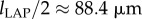was created, and the downsampling procedure (Gaussian filter and resampling) was applied to the test image (figure 7a). The sampling factor was calculated by dividing the pixel size of the test image by the pixel size of the LAP: f_s,LAP = 0.1 µm/64 µm. To reproduce the measured contrast of the line intensity profile (figure 7b), a Gaussian filter with a standard deviation of σ_PM = 45.7 µm was applied. To avoid boundary effects and ensure a symmetric line intensity profile, the dimensions of the image (1216 × 1216 µm) were chosen such that the downsampled image consists of an odd number of pixels (19 × 19 px).

Based on the determined parameters for the LAP (Δx_LAP, σ_LAP, f_s,LAP), downsampling parameters for imaging systems with other optical resolutions (table 1) were derived: the ratio between the pixel size of the LAP image and the determined standard deviation of the two-dimensional Gaussian filter is Analogous measurements of the PM yield a similar ratio between pixel size and standard deviation [36]. Assuming that this ratio is the same for all simulated imaging systems, the standard deviation of the two-simensional Gaussian filter was calculated from the pixel size Δx of the resulting downsampled image:

B 2

After applying the Gaussian filter, the synthetic image series (with pixel size Δx_sim) was resampled with a sampling factor of

B 3

yielding a downsampled image series with pixel size Δx.

Appendix C. Dependence of the phase shift on the local myelin thickness

Each myelin voxel of a simulated nerve fibre is represented by the Jones matrix of a rotated wave retarder as defined in equation (2.2). Depending on what kind of model is used (macroscopic or microscopic), the retarder axis is either oriented parallel or radially to the fibre axis (figure 2b).

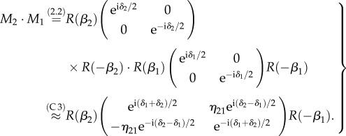
In the macroscopic model, the optic axes of the myelin voxels are all oriented in the fibre direction (φ, α) so that the voxels can be described by the same Jones matrix M_δ(β) with phase shift δ and . When the light propagates through N voxels of myelin, the multiplication of the N corresponding Jones matrices yields (using equation (2.2) and R(β)R(−β) = ):

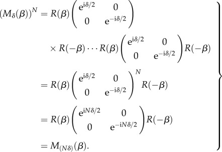C 1

Thus, the N myelin voxels with thickness Δt (along the optical path) and phase shift δ can be replaced by one myelin voxel with side length and phase shift:

C 2

In other words, the phase shift δ (and for small δ also the retardation ) scales linearly with the combined thickness of myelin voxels (NΔt), i.e. with the local myelin thickness t_m.

In the microscopic model, the optic axes of the myelin voxels along the optical path all have different orientations (φ_j, α_j) (figure 2c). If the optic axes of neighbouring myelin voxels have a similar direction ( and ), the multiplication of the N Jones matrices of the voxels can be simplified. For , one can define 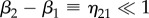and the multiplication of a pair of rotation matrices yields:

C 3

using a first-order approximation in η₂₁.

The multiplication of two Jones matrices yields (with ):

C 4

The multiplication of four Jones matrices yields (ignoring terms in the order of ):

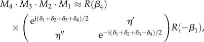C 5

where the elements of the secondary diagonal are given by

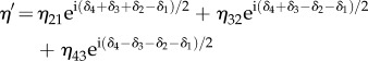C 6

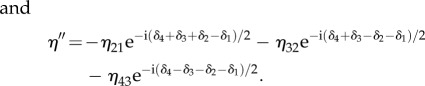C 7

If the number of myelin voxels (i.e. the number of matrices M_j) is small, the elements of the secondary diagonal in the resulting matrix can be neglected for . If the number of myelin voxels is large, the arguments of the exponential functions in the secondary diagonal will take all possible values and cancel each other for . In both cases, the multiplication of N Jones matrices yields:

C 8

Thus, the N myelin voxels with thickness Δt and phase shift δ_j can be replaced by one myelin voxel with thickness (NΔt = t_m) and phase shift:

C 9

given that the optic axes of neighbouring myelin voxels have similar directions.

The analytical considerations have shown that the phase shifts of individual voxels add together in both simulation models: in the macroscopic model, the phase shift scales linearly with the local myelin thickness t_m. In the microscopic model, this is only true for the upper limit of the phase shift. The dependence on the local myelin thickness is taken into account in the myelin density correction (see §3.5).

Appendix D. Retardation images of the fibre bundle

Figure 8.

Figure 8.

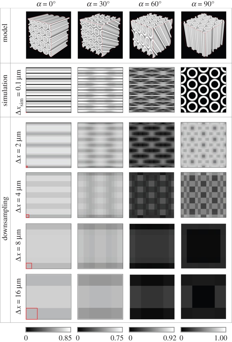
Retardation images of the hexagonal fibre bundle for selected fibre inclination angles α, simulated according to the microscopic model. The retardation values have been computed from (downsampled) image series with different pixel sizes Δx (according to table 1) after the myelin density correction. The pixel sizes are indicated by a square in the left bottom corner of the retardation images. To enhance the image contrast, a different scale bar is used for each inclination angle (the minimum value of the high-resolution retardation image is encoded in black, the maximum value in white). (Online version in colour.)

Authors' contributions

M.M. substantially contributed to the conception and design of the study as well as to the acquisition, analysis and interpretation of the simulated data. She carried out the simulations as well as the analytical calculations and drafted the manuscript. K.M. participated in the design of the study, contributed to theoretical considerations and to the interpretation of the simulated data, and helped draft the manuscript. H.D.R. contributed to the interpretation of the simulated data, to the theoretical considerations and to the revision of the manuscript. J.R. conducted experimental measurements, helped transfer the measurement results to the simulation and revised the manuscript. K.A. contributed to the anatomical content of the study and to the revision of the manuscript. M.A. coordinated the study, participated in the conception and design, contributed to the analysis and interpretation of the simulated data, and helped draft the manuscript. All authors read the final manuscript and gave final approval for publication.

Competing interests

We declare we have no competing interests.

Funding

This work was supported by the Helmholtz Association portfolio theme ‘Supercomputing and Modeling for the Human Brain’ and by the European Union Seventh Framework Programme (FP7/2007-2013) under grant agreement no. 604102 (Human Brain Project).

References

- 1.Behrens TEJ, Sporns O. 2012. Human connectomics. Curr. Opin. Neurobiol. 22, 144–153. ( 10.1016/j.conb.2011.08.005) [DOI] [PMC free article] [PubMed] [Google Scholar]
- 2.Sporns O, Tononi G, Kötter R. 2005. The human connectome: a structural description of the human brain. PLoS Comput. Biol. 1, 245–251. ( 10.1371/journal.pcbi.0010042) [DOI] [PMC free article] [PubMed] [Google Scholar]
- 3.Sporns O. 2009. The human connectome: linking structure and function in the human brain. In Diffusion MRI: from quantitative measurement to in vivo neuroanatomy (eds H Johansen-Berg, TEJ Behrens), pp. 309–332, 1st edn. Amsterdam, The Netherlands: Academic Press. [Google Scholar]
- 4.Axer M, Amunts K, Grässel D, Palm C, Dammers J, Axer H, Pietrzyk U, Zilles K. 2011. A novel approach to the human connectome: ultra-high resolution mapping of fiber tracts in the brain. NeuroImage 54, 1091–1101. ( 10.1016/j.neuroimage.2010.08.075) [DOI] [PubMed] [Google Scholar]
- 5.Axer M, et al. 2011. High-resolution fiber tract reconstruction in the human brain by means of three dimensional polarized light imaging. Front. Neuroinform. 5, 1–13. ( 10.3389/fninf.2011.00034) [DOI] [PMC free article] [PubMed] [Google Scholar]
- 6.Dohmen M, Menzel M, Wiese H, Reckfort J, Hanke F, Pietrzyk U, Zilles K, Amunts K, Axer M. 2015. Understanding fiber mixture by simulation in 3D polarized light imaging. NeuroImage 111, 464–475. ( 10.1016/j.neuroimage.2015.02.020) [DOI] [PubMed] [Google Scholar]
- 7.Göthlin GF. 1913. Die doppelbrechenden Eigenschaften des Nervengewebes—ihre Ursachen und ihre biologischen Konsequenzen. Kungl. Svenska Vet. Akad. Handlingar. 51, 1–91. [Google Scholar]
- 8.Schmitt FO, Bear RS. 1939. The ultrastructure of the nerve axon sheath. Biol. Rev. Camb. Phil. Soc. 14, 27–50. ( 10.1111/j.1469-185X.1939.tb00922.x) [DOI] [Google Scholar]
- 9.de Campos Vidal B, Silveira Mello ML, Caiseiro-Filho AC, Godo C. 1980. Anisotropic properties of the myelin sheath. Acta Histochem. 66, 32–39. ( 10.1016/S0065-1281(80)80079-1) [DOI] [PubMed] [Google Scholar]
- 10.Ambronn H. 1890. Das optische Verhalten markhaltiger und markloser Nervenfasern. Ber. K. Sächs. Ges. Wiss. Leipzi. Math-phys. Cl. 42, 419–429. [Google Scholar]
- 11.Darnell JE, Lodish HF, Baltimore D. 1990. Molecular cell biology. New York, NY: Scientific American Medicine. [Google Scholar]
- 12.Yuan A, Rao MV, Nixon V, Nixon RA. 2012. Neurofilaments at a glance. J. Cell Sci. 125, 3257–3263. ( 10.1242/jcs.104729) [DOI] [PMC free article] [PubMed] [Google Scholar]
- 13.Quarles RH, Macklin WB, Morell P. 2006. Myelin formation, structure and biochemistry. In Basic neurochemistry: molecular, cellular and medical aspects, (eds G Siegel, RW Albers, S Brady, D Price), pp. 51–71, 7th edn. Burlington, MA: Elsevier Academic Press. [Google Scholar]
- 14.Aggarwal S, Yurlova L, Simons M. 2011. Central nervous system myelin: structure, synthesis and assembly. Trends Cell Biol. 21, 585–593. ( 10.1016/j.tcb.2011.06.004) [DOI] [PubMed] [Google Scholar]
- 15.Martenson RE. 1992. Myelin: biology and chemistry. Boca Raton, FL: CRC Press. [Google Scholar]
- 16.Morell P, Quarles RH, Norton WT. 1989. Formation, structure, and biochemistry of myelin. In Basic neurochemistry—molecular, cellular, and medical aspects (ed. Siegel GJ.), pp. 109–136, 4th edn New York, NY: Raven Press. [Google Scholar]
- 17.Bear RS. 1971. The structure of the myelin sheath. Optical studies. Neurosci. Res. Program Bull. 9, 507–510. [PubMed] [Google Scholar]
- 18.Bear RS, Schmitt FO. 1936. The optics of nerve myelin. J. Opt. Soc. Am. 26, 206–212. ( 10.1364/JOSA.26.000206) [DOI] [Google Scholar]
- 19.Huang X-R, Knighton RW. 2005. Microtubules contribute to the birefringence of the retinal nerve fiber layer. IOVS 46, 4588–4593. ( 10.1167/iovs.05-0532) [DOI] [PubMed] [Google Scholar]
- 20.Oldenbourg R, Salmon ED, Tran PT. 1998. Birefringence of single and bundled microtubules. Biophys. J. 74, 645–654. ( 10.1016/S0006-3495(98)77824-5) [DOI] [PMC free article] [PubMed] [Google Scholar]
- 21.Koike-Tani M, Tani T, Mehta SB, Verma A, Oldenbourg R. 2013. Polarized light microscopy in reproductive and developmental biology. Mol. Reprod. Dev. 82, 548–562. ( 10.1002/mrd.22221) [DOI] [PMC free article] [PubMed] [Google Scholar]
- 22.Larsen L, Griffin LD, Grässel D, Witte OW, Axer H. 2007. Polarized light imaging of white matter architecture. Microsc. Res. Tech. 70, 851–863. ( 10.1002/jemt.20488) [DOI] [PubMed] [Google Scholar]
- 23.Jones RC. 1941. A new calculus for the treatment of optical systems. J. Opt. Soc. Am. 31, 488–503. ( 10.1364/JOSA.31.000488) [DOI] [Google Scholar]
- 24.Jones RC. 1942. A new calculus for the treatment of optical systems. J. Opt. Soc. Am. 32, 486–493. ( 10.1364/JOSA.32.000486) [DOI] [Google Scholar]
- 25.Collett E. 2005. Field guide to polarization. Washington, DC: SPIE—The International Society for Optical Engineering. [Google Scholar]
- 26.Glazer AM, Lewis JG, Kaminsky W. 1996. An automatic optical imaging system for birefringent media. Proc. R. Soc. Lond. A 452, 2751–2765. ( 10.1098/rspa.1996.0145) [DOI] [Google Scholar]
- 27.Aboitiz F, Scheibel AB, Fisher RS, Zaidel E. 1992. Fiber composition of the human corpus callosum. Brain Res. 598, 143–153. ( 10.1016/0006-8993(92)90178-C) [DOI] [PubMed] [Google Scholar]
- 28.Longstaff A. 2000. Neuroscience. New York, NY: Springer. [Google Scholar]
- 29.Hildebrand C, Remahl S, Persson H, Bjartmar C. 1993. Myelinated nerve fibers in the CNS. Prog. Neurobiol. 40, 319–384. ( 10.1016/0301-0082(93)90015-K) [DOI] [PubMed] [Google Scholar]
- 30.Schindelin J, et al. 2012. Fiji: an open-source platform for biological-image analysis. Nat. Methods 9, 676–682. ( 10.1038/nmeth.2019) [DOI] [PMC free article] [PubMed] [Google Scholar]
- 31.Müller H. 1943. Memorandum on the polarization optics of the photoelastic shutter. Report No. 2 of the OSRD project OEMsr-576.
- 32.Duck FA. 1990. Physical properties of tissue: a comprehensive reference book. New York, NY: Academic Press. [Google Scholar]
- 33.Beuthan J, Minet O, Helfmann J, Herrig M, Müller G. 1996. The spatial variation of the refractive index in biological cells. Phys. Med. Biol. 41, 369–382. ( 10.1088/0031-9155/41/3/002) [DOI] [PubMed] [Google Scholar]
- 34.Born M, Wolf E. 2011. Principles of optics—electromagnetic theory of propagation, interference and diffraction of light, 7th edn Cambridge, UK: Cambridge University Press. [Google Scholar]
- 35.Ghosh N, Vitkin IA. 2011. Tissue polarimetry: concepts, challenges, applications, and outlook. J. Biomed. Opt. 16, 110801 ( 10.1117/1.3652896) [DOI] [PubMed] [Google Scholar]
- 36.Reckfort J, Wiese H, Dohmen M, Grässel D, Pietrzyk U, Zilles K, Amunts K, Axer M. 2013. Extracting the inclination angle of nerve fibers within the human brain with 3D-PLI independent of system properties. In SPIE pro., polarization science and remote sensing VI, vol. 8873 (eds Shaw JA, LeMaster DA). San Diego, CA: SPIE–The International Society for Optical Engineering. ( 10.1117/12.2023198) [DOI] [Google Scholar]