Computational Calorimetry: High-Precision Calculation of Host–Guest Binding Thermodynamics

Abstract

We present a strategy for carrying out high-precision calculations of binding free energy and binding enthalpy values from molecular dynamics simulations with explicit solvent. The approach is used to calculate the thermodynamic profiles for binding of nine small molecule guests to either the cucurbit[7]uril (CB7) or β-cyclodextrin (βCD) host. For these systems, calculations using commodity hardware can yield binding free energy and binding enthalpy values with a precision of ∼0.5 kcal/mol (95% CI) in a matter of days. Crucially, the self-consistency of the approach is established by calculating the binding enthalpy directly, via end point potential energy calculations, and indirectly, via the temperature dependence of the binding free energy, i.e., by the van’t Hoff equation. Excellent agreement between the direct and van’t Hoff methods is demonstrated for both host–guest systems and an ion-pair model system for which particularly well-converged results are attainable. Additionally, we find that hydrogen mass repartitioning allows marked acceleration of the calculations with no discernible cost in precision or accuracy. Finally, we provide guidance for accurately assessing numerical uncertainty of the results in settings where complex correlations in the time series can pose challenges to statistical analysis. The routine nature and high precision of these binding calculations opens the possibility of including measured binding thermodynamics as target data in force field optimization so that simulations may be used to reliably interpret experimental data and guide molecular design.

1. Introduction

The rational design of high-affinity ligands, in applications like drug discovery and supramolecular chemistry, depends on an understanding of how interactions involving the ligand, receptor, and solvent contribute to the overall observed affinity. Calorimetric studies, which break down the binding affinity into enthalpic and entropic components, have been helpful in this respect and have led to discussions of entropy–enthalpy compensation¹⁻⁸ and the role of entropy and enthalpy in ligand design.⁹⁻¹⁵ Molecular simulations offer additional insight, as they link atomistic detail and binding thermodynamics, but, although decompositions of computed binding free energies into enthalpic and entropic terms are sometimes performed,¹⁶⁻¹⁹ this practice is not common, perhaps because these terms are regarded as being more difficult to compute. Importantly, simulations often allow the thermodynamic components themselves to be further subdivided to provide rich detail regarding the driving forces of the binding interaction, as we recently demonstrated for the binding enthalpies of a series of host–guest systems.²⁰

Here, we extend our previous work to describe what may be termed computational calorimetry, in which both a binding free energy and a binding enthalpy are obtained self-consistently from the same set of simulations. We focus on host–guest systems (Figure 1) for which ample experimental data are available²¹⁻³⁰ and extensive sampling can be achieved via GPU-enabled simulations.³¹ For these systems, just a few days of computing on commodity hardware yields numerical precision as good as or better than the corresponding reported experimental uncertainties. This precision is enabled, in part, by enhancements to the attach–pull–release (APR) free energy framework, which include the addition of orientational and conformational restraints that facilitate efficient simulations. As the centerpiece of this study, we validate the self-consistency of this approach by demonstrating excellent agreement between binding enthalpies computed directly, via end-state mean potential energies,^{16−20,32−34} and indirectly, via a van’t Hoff fit of the binding free energy.^16−19,35 Furthermore, we compare the numerical efficiency of these direct versus van’t Hoff approaches, determine whether hydrogen mass repartitioning (HMR) simulations³⁶⁻³⁸ can be used to speed the calculations without impacting their fidelity, and compare the results from two widely used approaches to estimate the statistical uncertainty of mean quantities from simulations with correlated data sets: statistical inefficiency analysis³⁹ and blocking analysis.⁴⁰

Figure 1.

Structures of the host (left) and guest (right) molecules studied in this work. The protonation state used in this study is shown for each guest and reflects the dominant species under experimental conditions. Binding thermodynamic values were calculated for cucurbit[7]uril (CB7) with all guests except Hex and for β-cyclodextrin (βCD) with Hex.

Comparison of our results with experiment reveals significant deviation. The extensive sampling and uncertainty analysis we perform, coupled with the relative simplicity of host guest systems, rules out sampling error as a major contributor to the deviation. Rather, to build rational explanations of binding, further testing and improvement of simulation force fields will be necessary. The computational calorimetry framework we describe will be helpful in performing such validation and development studies.

2. Methods

2.1. Binding Systems

The model host–guest systems we chose for this work, cucurbit[7]uril (CB7) and β-cyclodextrin (βCD), exemplify key features of protein–ligand binding, but they are far more computationally tractable due to their small size. The two hosts differ in their conformational properties and binding characteristics. CB7 systems feature high binding affinities^24,27,41 and thus require a rigorous approach to deal with the steep energy landscape encountered when removing the guest. Additionally, binding enthalpies have been previously calculated²⁰ for these systems using the same force field parameters but with a different simulation box setup, thus providing a convenient comparison to study the influence of the choice in setup, as detailed below. Cyclodextrin host–guest systems are attractive due to the wealth of experimental data available.²¹⁻²³ Although their binding affinities tend to be more modest than those of CB7 systems, their flexibility and large number of hydrogen-bond donors and acceptors offer a potentially more realistic representation of protein–ligand binding. A complicating issue with cyclodextrins is that many guest molecules can bind in two orientations that do not exchange on the microsecond time scale of the present simulations. For example, hexanoate can bind to βCD with the carboxylate group near the primary hydroxyl face (primary binding mode) or at the secondary hydroxyl face (secondary binding mode). Thus, binding calculations must be performed for both orientations and combined to yield a single value (see Section 2.2.3). Finally, we study an extremely simple model of binding, an ion-pair, to validate our computational procedures at high precision.

The following subsections describe the parametrization and system building protocol. Each set of simulations is named according to the binding pair; the subscript Temp indicates a temperature series used for van’t Hoff binding enthalpy calculations, and the subscript HMR indicates calculations using hydrogen mass repartitioning. Refer to Figure 1 and Table 1 for illustrative and technical summaries, respectively, of the simulation sets discussed below.

Table 1. Simulation Sets Studied in This Work.

simulation set	setup detailsa	values calculated	total time (ns)b
CB7-All8	I	ΔG: 8 guests at 300 K	35265
		ΔH: 8 guests at 300 K	16000
CB7-B2Temp	I	ΔG: 282, 288, 294, 300, 306, 312, 318 K	111090
		ΔH: 300 K	3000
CB7-B2HMR	I	ΔG: 300 K	13094
		ΔH: 300 K	4000
βCD-HexTemp	I	ΔG: 280, 290, 300, 310, 320 Kc	174536
		ΔH: 300 Kc	33849
βCD-HexHMR	I	ΔG: 298 Kc	16 955
		ΔH: 298 Kc	16955
βCD-HexAlt	I	ΔG: 300 Kd	13 958
		ΔH: 300 Kd	2000
K-ClSimple	II	ΔG: 300 K	4000
		ΔH: 300 K	2000
K-ClTemp	III	ΔG: 280, 290, 300, 310, 320 K	69563
		ΔH: 300 K	2312

^aSimulation setup types are as following: I = Rectangular box with a 3 anchor particle restraint setup; II = Truncated octahedron box with 1 distance restraint; III = Rectangular box with a two anchor particle restraint setup.

^bAggregate simulation time over the entire simulation set is indicated for direct calculations of the binding free energy and binding enthalpy. Note that the binding free energy total time includes the binding enthalpy simulation time since the latter can be included with the former.

^cFree energies and enthalpies were determined for the guest in two orientations inside the βCD host, requiring twice as many simulations. Additionally, the total time listed for the ΔH includes the two free energy calculations required to appropriately weight the contributions from the two binding orientations.

^dCalculations were performed only on the primary orientation, as these simulations served as a consistency check.

2.1.1. Cucurbituril Host and Eight Guests

All CB7 simulation sets used the same parameters as those described by Fenley et al.²⁰ in order to maintain consistency with that publication. Briefly, parameters for the CB7 host and the guests were assigned by the program Antechamber:⁴² partial charges used the AM1-BCC method,^43,44 whereas bonded and nonbonded parameters came from GAFF.⁴⁵ All simulations (both bound and unbound) were solvated in an orthorhombic box of 2210 TIP3P waters with dimensions of approximately 36 × 36 × 52 ų, with the exception of the larger B11 guest, for which 2500 waters were used in a box of dimensions 36 × 36 × 60 ų. The simulation with the MVN guest also included one molecule of protonated Tris buffer in order to match experiment. Included in each simulation box were three noninteracting anchor particles, which, in conjunction with several restraints, aligned the host–guest system with the long axis of the box. Hydrogen mass repartitioning was tested for the association of CB7 with B2. For these CB7-B2_HMR simulations, the parameter/topology file was modified with the Parmed.py program (distributed with AMBER) to reallocate the solute atom masses in accordance with previously described hydrogen mass repartitioning schemes.³⁶⁻³⁸ Solvent molecules were not modified.

2.1.2. β-Cyclodextrin Host and Hexanoate Guest

Cyclodextrin parameters were taken from Cézard et al.,⁴⁶ and hexanoate parameters used RESP⁴⁷ partial charges from the R.E.D. Server program^48,49 and other bonded/nonbonded parameters from GAFF.⁴⁵ In an attempt to closely match typical experiments, which include 10–20 mM phosphate buffer, we included two molecules each of H₂PO₄^– and HPO₃^2– and neutralized with an appropriate number of sodium ions. To our knowledge, there are no established parameters for inorganic phosphate ions in the AMBER community, so we began with parameters for existing bio-organic phosphates. Partial charges for each species were determined with a RESP fit while Lennard-Jones terms and bonded parameters were taken from GAFF. Because we observed nonphysical aggregation of phosphate and sodium ions in the initial simulations, we increased the Lennard-Jones radius parameters for the phosphate oxygen atoms from their default values by 0.29 and 0.33 Å for H₂PO₄^– and HPO₃^2–, respectively, in accordance with conclusions from Steinbrecher et al.⁵⁰ This change eliminated the aggregation, but we do not regard these parameters as optimal, and we note the caution from Steinbrecher et al. in regards to the uncertainty of their suitability. The entire system was solvated with 2210 TIP3P waters in an orthorhombic box whose dimensions were approximately 36 × 36 × 52 ų. As for the CB7 simulations, anchor particles were used to orient the system along the long axis of the box. Calculations were done with (βCD-Hex_HMR) and without (βCD-Hex_Temp, βCD-Hex_Alt) hydrogen mass repartitioning of the solute.

2.1.3. Ion-Pair Test Case

As a toy system that would allow unambiguous numerical convergence, and thus rigorously test our computational setups, we studied the binding of two monatomic ions in aqueous solution. We used a single K⁺ and Cl^– ion pair, with cation parameters from Åqvist⁵¹ and anion parameters from Dang,⁵² but we modified the ion parameters to create a diatomic system with favorable enough affinity to bind together during simulation. In particular, although this combination is known to produce unphysical ion pairing,⁵³ the binding was not sufficiently tight to mimic a host–guest-like system, so we increased the binding affinity by artificially changing the charges on each ion from ±1.0 to ±1.3. This led to a fairly stable ion pair, which persisted during simulation. The K-Cl_Simple simulation set, which did not include orienting anchor particles (see Section 2.5), was solvated with 2000 TIP3P waters in an isotropic truncated octahedron. In contrast, the K-Cl_Temp simulations, which did use orienting anchor particles, were solvated with 1000 TIP3P waters in an orthorhombic box with dimensions of approximately 25 × 25 × 50 ų, where the long dimension of the box corresponds to the guest pulling axis.

2.2. Binding Free Energy Calculations

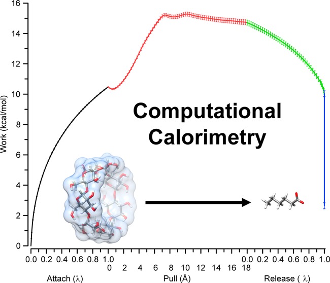
Our general approach to free energy calculations extends the theoretical framework described by Velez-Vega and Gilson,⁵⁴ in which the binding free energy is computed in terms of the sum of the work, W, required to attach restraints to the complex, pull the ligand from the binding site and then release the attached restraints (see schematic summary in the left-hand panel of Figure 2):

1

Here, rather than performing a single dynamic pulling calculation, we break the calculation into a series of independent simulation windows. The collection of independent simulations can still be viewed as spanning an attach–pull–release (APR) process, although, due to their independent nature, the process could be equally viewed as unrelease–push–unattach. Breaking the free energy path into independent simulations has two advantages: (1) because each simulation is independently built and equilibrated, little or no memory effect is encountered from one point on the path to the next; (2) the entire calculation can be distributed across a large, heterogeneous computational cluster, in order to improve turnaround. In the following subsections, we provide more detail on the binding free energy calculations performed in this work, starting with a thermodynamic integration (TI) approach for calculating the binding free energy from the APR simulation data.

Figure 2.

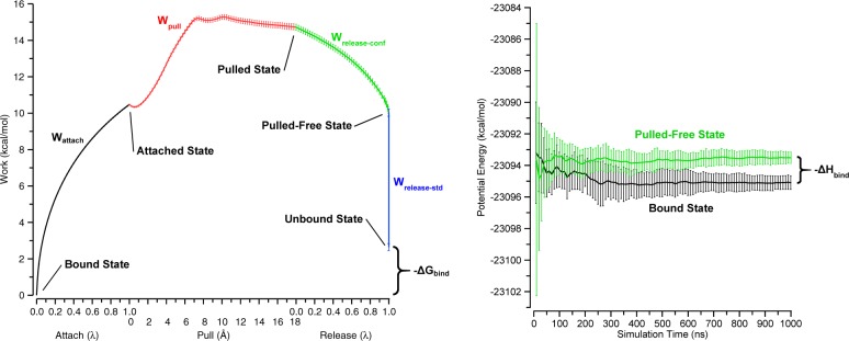
Depiction of the attach–pull–release (APR) binding free energy calculation (left) and the direct binding enthalpy calculation (right). The data shown was obtained from the primary orientation of the βCD-Hex_Temp simulation set at 300 K. Error bars are 95% CI.

2.2.1. Thermodynamic Integration Approach

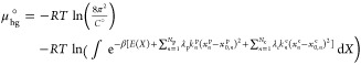
Following the approach detailed by Velez-Vega et al.,⁵⁴ we first define the chemical potential of the restrained host–guest system in the following manner

2

where β ≡ 1/RT, R is the gas constant, T is the absolute temperature, C° is the standard concentration (1 M or 1 particle/1660 ų), and E(X) is the potential energy as a function of atomic coordinates, X, defined in the reference frame of the host. The equation includes two nonphysical summation terms that define harmonic restraint potentials on the rotational and translational coordinates, or pose, of the guest relative to the host, x_n^p, and on a set of conformational coordinates internal to the host and/or the guest, x_n. The N_p/N_c number of harmonic restraints are described with force constants, k_p/k_c (which implicitly include a factor of 1/2, according to the convention in AMBER), and target values, x_0,n^p/x_0,n, along with scaling coefficients λ_p/λ_c, which are varied from 0 to 1 in order to turn the restraints on and off in the course of the free energy calculations. In addition, E(X) implicitly includes a set of energy terms that restrain the overall translational and rotational coordinates of the host within the lab frame, without influencing its conformational distribution. These restraints remain in place and unchanged during the entire APR process. Most simply, a single atom of the host may be restrained to a lab-frame position. More generally, it may be convenient to keep the host positioned in and aligned with the long axis of a rectangular simulation box via restraints tied to a set of artificial particles anchored in the lab frame (black restraints in the Figure S1A example).

In the following sections, we will refer to five host–guest states, which depend on the status of the variable restraints: bound, attached, pulled, pulled-free, and unbound. These states are illustrated in Figures 2 (left panel) and S1. The bound state has the guest bound to the host but with no added restraints. The attached state is the same, except that restraints have been turned on. In the pulled state, the restraints are still on, but the equilibrium value of the restraint that sets the host–guest distance has been adjusted to keep the guest far from the host. In the pulled-free state, the conformational restraints have been turned off, but the pose restraints are still in force. In the unbound state, the pose restraints are removed and the guest is considered to be at the standard state concentration. The following sections explain the process for moving the host–guest system through each of these states.

2.2.1.1. Attachment Phase

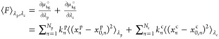
This phase begins with the system in the bound state. The bound state does not include rotational or translational restraints on the guest or conformational restraints on either the host or the guest. Therefore, using the definition in eq 2, the bound state corresponds to λ_p = 0 and λ_c = 0. With λ_p = 1 and λ_c = 1, the chemical potential is defined as the attached state, as it now includes restraints necessary to extract the guest (depicted in gray in the Figure S1B example). The force of attaching these restraints is λ-dependent and can be found by taking the partial derivative of μ_hg^° with respect to λ_p and λ_c (intermediate steps given in Supporting Information).

3

Note that the angle brackets indicate the mean value from the simulation at a given value of λ_p/λ_c. Also, the scaling of λ_p/λ_c should be performed simultaneously for the above equation to be valid. To compute the work, we estimate the integral over the force curve (Figure 2, left)

4

from a series of simulations with discrete λ steps from 0 to 1, as detailed in the Appendix.

2.2.1.2. Pulling Phase

The geometry of the host molecule and our restraint setup (Figure S1B) allows us to vary the target value of a single distance restraint parameter, designated x_0,1^p in our general equations below, in order to pull the guest away from the host while the other restraints remain constant. At this point, all of the restraints are fully turned on (λ_p = λ_c = 1), and we compute the work of increasing x_0,1 from its initial to its final value, which is the pulled state (Figures 3 and S1C). First, we write the mean force as the partial derivative of the chemical potential with respect to the varying parameter, x_0,1^p (see intermediate steps in Supporting Information):

5

Note that, during the pulling phase, usually x_0,1^p > ⟨x₁⟩, so the present expression will generally yield a positive work for pulling the guest from the host, as expected for favorable binding. To find the work, we integrate the force over the change in equilibrium restraint length from the initial attached distance to a final pulled distance at which the host and guest can be considered to be noninteracting.

6

As in the attachment phase, in practice the integration is estimated from simulations at discrete steps in x_0,1^p.

Figure 3.

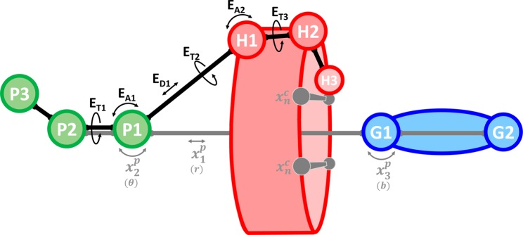
Restraint scheme demonstrating the use of anchor particles for attach–pull–release (APR) free energy calculations. P1–3 are anchor particles, H1–3 are host atoms, and G1–2 are guest atoms. The E_D1, E_A1–2, and E_T1–3 labels indicate distance, angle, and torsion restraints, respectively, which modify only the host translational and rotational degrees of freedom and are included implicitly in the potential energy function, E(X), as described in the main text. These restraints are held constant throughout all simulation windows and do not perturb the host’s conformational degrees of freedom. Indicated in gray with labels x₁^p, x₂, x₃^p, and x_n are restraints that are attached over a series of simulation windows and are subsequently used to pull the guest out of the host cavity. In this example, x₁^p is a distance restraint, x₂ and x₃^p are angle restraints, and x_n represents host conformational restraints (of any harmonic form). In parentheses, the corresponding spherical coordinate or Euler angle is indicated for each translational/rotational pose restraint, as defined in the main text. See Figure S1 for a full illustration of the APR process.

2.2.1.3. Release Phase

In the release phase, all of the restraints added during the attachment phase must be removed either by numerical integration or analytically. Those restraints that perturbed the conformational distribution of the system, either host or guest, are removed in precisely the same manner as the attachment phase, except that now the guest is held far from the host. In this case, only λ_c is varied, while the scaling factor for the translational and rotational pose of the guest relative to the host, λ_p, is held constant. The λ-dependent force curve is integrated and multiplied by −1 to find the work of releasing the N_c conformational restraints.

7

After removal of the conformational restraints, the system is in the pulled-free state (Figure S1D). Note that, in cases where conformation-perturbing restraints are not used, there is no distinction between the pulled and pulled-free states.

Finally, since the guest’s rotational and translational degrees of freedom are still restrained relative to the frame of reference of the host, we calculate the work to release these restraints and place the guest at standard concentration (the unbound state, depicted in Figure S1E). This work is the difference between the chemical potential of the pulled-free state and the sum of the chemical potentials of the separate host and guest at standard concentration:

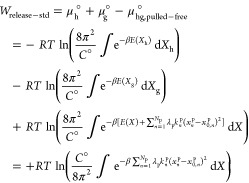8

Here, X_h and X_g represent the coordinates of the host and guest respectively, so that X = (X_h,X_g). The cancellation of the energy potential term is dependent on the assumption that the host and guest are far enough apart to be noninteracting so that E(X) = E(X_h) + E(X_g). For evaluation of the W_{release–std} term, it is helpful to reconsider the guest’s translational degrees of freedom in the spherical coordinate system (r, θ, φ) and its orientation in terms of Euler angles (a, b, c). Here, we rewrite eq 8 with appropriate Jacobian terms and, in accordance with our example figures, identify the two translational restraints as r and θ and one rotational restraint as b:

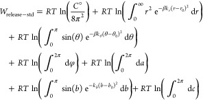9

This equation can be evaluated semianalytically, without the use of molecular simulations. Note that it may readily be generalized to a calculation in which restraints are also applied to φ, a, and/or c.

2.2.2. Multistate Bennett Acceptance Ratio Approach

One may use the same set of dynamics trajectories to compute W_attach, W_pull, and W_{release–conf} values by the MBAR estimator approach.⁵⁵ (W_{release–std} is still computed semianalytically, as noted above.) This is done by postprocessing the simulation trajectories to obtain the restraint potential energy of each simulation frame in the restraint potential of each simulation window. The freely available Pymbar implementation of the MBAR estimator⁵⁵ can then be used to determine the relative free energy along the entire free energy path.

2.2.3. Multiple Non-exchanging Bound States

For some host–guest complexes, the guest can adopt multiple, distinct orientations that do not readily convert without unbinding. For example, an asymmetric guest may bind to β-cyclodextrin head-in or head-out. In such cases, the overall binding free energy can be computed from N_b separate binding free energies of the N_b noninterconverting configurations:

10

Note that eq 10 places greater weight on results of lower free energy, so errors in the component free energies propagate nonlinearly. Therefore, we estimate both the mean and the uncertainty of ΔG_bind,all^° by numerically sampling from a Gaussian distribution based on the values of ΔG_bind,n and their respective uncertainties (see Appendix).

2.3. Binding Enthalpy Calculations

The enthalpy calculations in this article are performed in one of two ways, termed the direct and van’t Hoff methods,¹⁶⁻¹⁹ as now detailed.

2.3.1. Direct Method

The binding enthalpy is the difference between the partial molar enthalpies of the complex and the free molecules. In the direct approach, this quantity is obtained from differences in mean potential energy between simulations of the bound and free states. (Note that the pressure–volume contribution to the binding enthalpy is negligible for binding in solution.) Previously, Fenley et al.²⁰ implemented this method by a multi-box approach, which uses four separate simulations of the free host, the free guest, the host–guest complex, and any additional pure solvent needed to exactly balance the stoichiometry of the bound and unbound simulations. Here, we instead use a single-box approach, which involves simply subtracting the mean energy of the host–guest system in the pulled-free state from that of the bound complex (Figure 2, right)

11

where U is defined as the potential energy without any restraining potentials included. It should be emphasized that, in these bound and pulled-free states, the restraining potentials have no influence on the internal coordinates of the molecules. In the pulled-free state, they only hold the host and guest far apart, along an axis aligned with the long axis of the rectangular simulation box. The two states considered here correspond to simulations in the first (Figure S1A) and last (Figure S1D) simulation windows of the APR binding free energy approach. As shown in Results, this single-box method gives excellent agreement with the prior multi-box approach.

When N_b noninterchangeable binding orientations exist, as for the present βCD systems, where N_b = 2, the binding enthalpy of the various orientations must be weighted by their respective free energies to yield the overall binding enthalpy:

12

Again, this combination step is carried out using resampling from Gaussian distributions based on the mean and SEM of each input value.

2.3.2. van’t Hoff Method

This approach involves using the van’t Hoff equation or related forms to extract the binding enthalpy and entropy from calculations of the binding free energy (described above) at multiple temperatures. If one makes the approximation that enthalpy and entropy are invariant with temperature, then both values can be obtained by fitting to the familiar integrated form of the equation

13

via linear regression analysis on a plot of ln(K_eq) versus 1/T. Here, however, we allowed for temperature dependence by explicitly including a fitted change in the heat capacity, ΔC_p, using the following equation, where the thermodynamic parameters were fitted with nonlinear curve fitting tools:³⁵

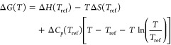14

Here the ref subscripts indicate the reference temperature for which the parameters are fitted. We used simulations to compute ΔG(T_i) at either five or seven different temperatures, T_i, at uniform temperature intervals and with a central temperature (i = 3 or i = 4, respectively) of 300 K; chose T_ref = 300 K; and used the values of ΔG(T_i) at all five or seven temperatures to fit the values of ΔH(T_ref), ΔS(T_ref), and ΔC_p(T_ref) via nonlinear fitting. It is worth remarking that this approach yielded a value of ΔH(T_ref) that was statistically indistinguishable from that obtained by using eq 13 as mentioned above. On the other hand, a pure finite difference method, in which the entropy or enthalpy is computed from just two free energy values at nearby temperatures, results in very large uncertainties, as may be appreciated by inspection of the data in the top panels of Figure 7. Thus, numerical uncertainty is substantially decreased by using free energies computed at multiple temperatures, as done here.

Figure 7.

Demonstration of the temperature dependence of the binding free energy (top) and the convergence of the van’t Hoff and direct binding enthalpy calculations at 300 K (bottom). Data is shown for the CB7-B2_Temp (left) and βCD-Hex_Temp (right) simulation sets. Error bars are 95% CI.

2.4. Quantifying Statistical Uncertainty

We use numerical molecular simulations to estimate the mean quantities in the equations above, so the reported binding enthalpies and free energies are estimates associated with statistical uncertainties, in the sense that replicating the simulations with slightly different starting conditions or random number seeds would yield somewhat different means, given finite sampling. It is possible to estimate the uncertainty of the mean without actually running time-consuming replicates so long as time correlation within the simulation data is accounted for properly.⁵⁶ We investigated two approaches. First, the blocking method⁴⁰ iteratively averages a time course data series (e.g., the potential energy, in an enthalpy calculation) into successively larger blocks and calculates the SEM of the block averages at each block size. The resulting plot of block size versus SEM will, ideally, display a plateau feature in the curve. The SEM value of the plateau region is an error estimate that accounts for correlation in the data. However, it is not straightforward to automate detection of a plateau, and, in some cases, there is no clear plateau, as detailed in Section 3.5. Therefore, in order to automate the usage of this method, we conservatively chose to use the maximum SEM value obtained by the blocking analysis, even if it comes from the noisy region of very large block sizes at the far right of the graph rather than from a plateau region. Second, the statistical inefficiency³⁹ (StIn) method involves estimating the autocorrelation function of the data series. The effective number of uncorrelated data points is then found by dividing the total number of correlated data points by the StIn value. The usual formula for the SEM of an uncorrelated data series can then be used. Following what has been presented in the literature, we couple the TI free energy calculations with the blocking method and the MBAR calculations with the StIn method (although any combination could be used). A comparison of these approaches is presented in the Results. Further description of the error propagation in each value calculated is given in the Appendix.

2.5. Restraint Setup

In order to perform the binding free energy calculations described in this work, restraints must be used to guide the host and guest apart along a free energy path. In one case (K-Cl_Simple), we used a single distance restraint between the ions, primarily as a reference benchmark for more complicated but efficient restraint schemes that control the position and orientation of the pulling axis. We discuss the restraint setup details for each simulation set (Table 1) in the following text.

2.5.1. Orientation with Anchor Particles

Many of the simulations we present include 2 or 3 noninteracting anchor particles, which are positionally restrained to fixed Cartesian coordinates. The anchor particles have zero charge, zero Lennard-Jones radius and well-depth, and a mass of 220 Da. To these anchor particles we attach harmonic distance, angle, and torsion restraints that position and orient the host and guest. Figures 3, S1, and S2 diagram a typical anchor particle restraint setup for a host–guest system and an ion-pair toy model. For the ion-pair simulations, we use two restraints per ion: a distance restraint and an angle restraint set to 180°. This combination effectively locks all three translational degrees of freedom. Six restraints are required to control the three translational and three rotational degrees of freedom of the polyatomic hosts. These include one distance restraint, two angle restraints, and three torsional restraints; similar restraint sequences have been described previously.⁵⁷ It is critical to note that, in order for the binding free energy results to be valid, these six restraints must be designed so that they do not perturb the conformational distribution of the host molecule; see, e.g., Figure S1A. These host restraints are present during the entire APR process, from the beginning to the end; thus, they are not imposed during the attach phase or detached during the release phase. In all cases with anchor particles, except the βCD-Hex_HMR simulation set, the host translational and rotational restraints had the following force constants: distance restraints used a 10.0 kcal/mol·Å² force constant, whereas angle and torsional restraints used 100 kcal/mol·rad². A weaker distance restraint force constant of 5.0 kcal/mol·Å² was tested for the βCD-Hex_HMR simulation set, whereas the other force constants were identical, but no difference was observed. The target equilibrium values of these host restraints were set equal to the initial values of the input structure, which was manually oriented in UCSF Chimera.⁵⁸

2.5.2. Host Conformational Restraints

In all simulations involving CB7 and βCD, restraints were added during the attachment phase to adjust and restrain the host conformation in a manner that would facilitate sampling during the pulling phase. This approach is conceptually similar to the confine-and-release method that has been described for alchemical free energy calculations of protein–ligand complexes.⁵⁹ The CB7 host, which is a very stiff molecule with narrow entry portals, poses a high energetic barrier to removing guests from its cavity. We used 14 distance restraints, seven spanning each of the cavity portals, to enlarge the cavity opening and reduce the energy barrier for guest removal (Figure S3). The work of adding these restraints is relatively easy to converge, and opening the portal in this manner avoids sampling problems that would otherwise occur during the pulling phase, as the guest pops like a cork from the restrictive portal.^54,60 In contrast to the CB7 molecule, βCD is very flexible and can get dragged into distorted conformational substates for many nanoseconds as it clings to the guest during the pulling-phase simulations; the associated fluctuations and conformational trapping can make convergence difficult. To alleviate this problem, 14 torsional restraints (two per glucopyranoside monomer) were added to the β-cyclodextrin backbone during the attachment phase of the free energy calculation. The effect of these restraints is to maintain the symmetrical, canonical shape of the βCD molecule. The work of adding these restraints is easy to converge, as the host’s conformation does not fluctuate much in the presence of the bound guest. Overall, the present restraint schemes significantly improve the reproducibility of the calculated binding free energies for the systems we have tested.

Additionally, the work of releasing such conformational restraints must be included in the release phase, with the guest now far from the binding site. We accomplished this by performing the exact same simulations as the attachment phase except the guest is either held at a constant remote distance (in the case of the CB7-B2_Temp, CB7-B2_HMR, and βCD-Hex_Alt simulation sets) or removed entirely from the simulation (all other CB7 and βCD simulation sets). In the latter cases, we added a single simulation window of the guest in the pulled-free state with host conformational restraints released (Figure S1D) in order to compute the direct enthalpy.

2.5.3. Guest Restraints

Fewer restraints were required to orient the guest molecules on the pulling axis. Control of the necessary degrees of freedom was achieved with just two or three restraints for the ion-pair and host–guest systems, respectively, due to convenient properties of 180° angle restraints. We note here that it was necessary to include constant flatwell restraints during the attachment phase for the weaker affinity systems in order to prevent occasional dissociation of the bound complex. An arbitrary choice must be made about where to place the boundary of the bound state in these cases.

The details of the guest restraints and chosen number of windows for each calculation are given in the Supporting Information. Some of the details vary from one simulation set to another as we optimized our protocol during the course of this investigation. However, none of the changes were made due to concerns about the quality of a previously collected simulation set; rather, we optimized our overly conservative initial approach for the sake of greater computational efficiency.

2.6. Molecular Dynamics Simulation Details

All simulations were performed using the pmemd, pmemd.MPI, and pmemd.cuda programs from AMBER 14.⁶¹ Production simulations were run in the NPT ensemble, with temperature control using a Langevin thermostat⁶² with collision frequency 1.0 ps^–1 and pressure control provided by the Monte Carlo barostat⁶³ for all simulation sets except the CB7-B2_Temp, which used the Berendsen barostat⁶⁴ to check consistency with previous work²⁰ (note that we have not observed differences between the two barostats). Direct space nonbonded interactions were truncated with a 9.0 Å cutoff, whereas long-range electrostatics were handled with the PME method^65,66 using default AMBER settings. SHAKE constraints^67,68 were applied to bonds involving hydrogen, and the simulation time step was set to 2 fs, with the exception of HMR simulations, which used a 4 fs time step. Anchor particles, when present, were maintained at the desired coordinates using 100 kcal/mol·Å² positional restraints, except for the CB7-All8 and βCD-Hex_HMR sets, which used 50 kcal/mol·Å². The equilibration process consisted of the following steps: (1) minimization of the initial system with positional restraints maintained on the anchor particles, host, and guest, (2) 50 ps of NPT simulation at 50 K with the same positional restraints as the minimization, (3) 1.0 ns of NPT simulation with smooth heating from 50 K to the desired final temperature without positional restraints on the host or guest, and (4) 2.0 ns of NPT equilibration at the final temperature without positional restraints. Two strategies were employed to determine the length of the production simulations. For the CB7-B2_Temp set, we chose a fixed simulation length for each window involved in the APR path. For all other simulation sets, we chose a variable simulation length for each window that depended on either reaching a specified error value in the forces or reaching a maximum simulation time, whichever came first. The simulation windows for the bound and pulled-free states were then extended to at least 1 μs when the direct enthalpy calculation was required. For the HMR simulations, which have previously been reported,³⁶⁻³⁸ AMBER’s parmed.py program was used to edit the standard parameter/topology file in order to increase hydrogen masses to 3.024 Da and reduce the mass of neighboring heavy atoms accordingly. The water molecules were not altered.

3. Results

3.1. Computational Calorimetry

Computational calorimetry simulations were performed on nine host–guest systems for which experimental data are available (Table 2), using the attach–pull–release (APR) method for the free energy and the direct, single-box method for the binding enthalpy. The calculated binding thermodynamics display a strong tendency to overestimate the measured favorability of the binding free energy, the binding enthalpy, and the binding entropy (Table 2 and Figure 4). The RMSD values of these thermodynamic quantities, relative to experiment, are all greater than 4 kcal/mol, with the largest RMSD, ∼8 kcal/mol, observed for the binding free energies due to overestimation of both the enthalpic and entropic contributions. On the other hand, the computed binding free energy and enthalpy correlate well with experiment, with R² values of 0.92 ± 0.09 and 0.87 ± 0.17, which suggests that there may be a systematic cause for the large absolute deviations from experiment.

Table 2. Comparison of Experimental and Calculated Binding Data^a.

		ΔGbind		ΔHbind		–TΔSbind
simulation set	host, guest	experiment	calculated	experiment	calculated	experiment	calculated
CB7-All8	CB7, A1	–14.1 ± 0.2	–23.74 ± 0.29	–19.0 ± 0.5	–24.89 ± 0.43	4.9 ± 0.5	1.15 ± 0.52
CB7-All8	CB7, A2	–19.4 ± 0.1	–27.41 ± 0.27	–19.3 ± 0.5	–22.64 ± 0.60	–0.1 ± 0.6	–4.78 ± 0.66
CB7-All8	CB7, B2	–13.4 ± 0.1	–21.25 ± 0.22	–15.8 ± 0.2	–21.59 ± 0.41	2.4 ± 0.2	0.34 ± 0.47
CB7-All8	CB7, B5	–19.5 ± 0.2	–27.12 ± 0.36	–15.6 ± 0.5	–18.27 ± 0.48	–3.9 ± 0.6	–8.86 ± 0.60
CB7-All8	CB7, B11	–20.6 ± 0.5	–30.41 ± 0.81	–16.3 ± 0.5	–17.71 ± 0.48	–4.3 ± 0.6	–12.70 ± 0.94
CB7-All8	CB7, G8	–6.12 ± 0.12	–13.89 ± 0.29	–8.5 ± 0.6	–6.26 ± 0.48	2.4 ± 0.6	–7.63 ± 0.56
CB7-All8	CB7, G9	–7.43 ± 0.14	–18.49 ± 0.59	–3.8 ± 0.2	–11.68 ± 0.54	–3.6 ± 0.3	–6.81 ± 0.80
CB7-All8	CB7, MVN	–7.08 ± 0.14	–11.07 ± 0.68	–3.2 ± 0.2	–2.34 ± 0.53	–3.9 ± 0.1	–8.73 ± 0.86
βCD-HexTemp	βCD, Hex	–2.28 ± 0.07	–3.86 ± 0.17	1.31 ± 0.08	–1.13 ± 0.66	–3.59 ± 0.03	–2.73 ± 0.68
	RMSD	7.95 ± 1.50		4.19 ± 1.55		5.40 ± 1.92
	MSE	–7.48 ± 1.84		–2.92 ± 2.02		–4.56 ± 2.00
	MUE	7.48 ± 1.84		3.61 ± 1.47		4.75 ± 1.80
	R2	0.92 ± 0.09		0.87 ± 0.17		0.51 ± 0.49

^aExperiments were all ITC measurements. A1, A2, B2, B5, and B11²⁷ were at 298.15 K, G8 and G9⁴¹ were at 300 K, and MVN²⁴ was at 298 K. Data for MVN is an averaged obtained from the published value and two additional measurements via personal communication. All simulations were performed at 300 K. The calculated binding enthalpy was via the direct method. Calculated −TΔS was determined by subtracting the binding enthalpy from the binding free energy, and the uncertainty was determined by addition of the respective errors in quadrature. Uncertainty values for the thermodynamic data given as 95% CI calculated with the TI/blocking approach. The uncertainty in the error statistics are also 95% CI, determined by resampling the data with replacement.

Figure 4.

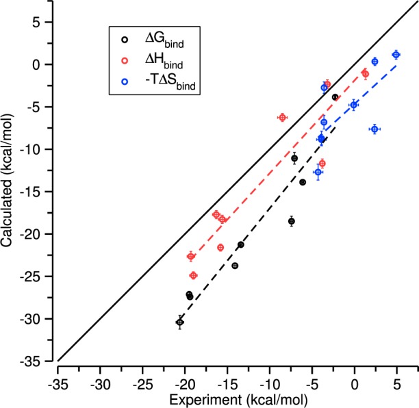
Comparison of the experimental and calculated binding values for the systems in Table 2. Error bars are 95% CI.

The statistical uncertainties of both the computed and the measured thermodynamic quantities are on the order of 0.5 kcal/mol (Table 2). As a consequence, the deviations of the calculations from experiment cannot be attributed to inadequate sampling during the molecular dynamics simulations. This view is supported by the highly stable convergence graphs shown in Figure 5; indeed, the binding free energies and enthalpies obtained with 100% of the simulation data in all cases remain within the confidence intervals obtained with only 10% of the data. Finally, inspection of the simulation trajectories suggests that good conformational sampling has been achieved. This is demonstrated in Figure 6, where we overlay the time-averaged structure for the bound state of every host–guest system reported in Table 2. Due to averaging of the guest’s orientation within the host, the extensive sampling results in a stick-like appearance of the guests inside the host; the averaging also gives the host a regular, symmetric appearance. In the case of CB7 with the aromatic guests, this differs substantially from the elliptical distortion characteristic of a typical instantaneous bound conformation. Likewise, the time-averaged βCD structure displays a uniform conformation for each glucopyranoside monomer, which contrasts with a typical instantaneous binding pose in which each monomer flexibly adopts its own conformation, producing an asymmetrical appearance. The thorough convergence and small statistical uncertainties of these results highlight the feasibility of performing numerically precise computational calorimetry studies on host–guest systems.

Figure 5.

Convergence plot of the binding free energy and binding enthalpy for the systems in Table 2. The guests are indicated in the legend at right. CB7 was the host molecule for all guests except Hex, which bound to βCD. Convergence is indicated by percentage of total data due to the varying trajectory length of the simulation windows considered in the ΔG_bind or ΔH_bind calculations. Error bars are 95% CI.

Figure 6.

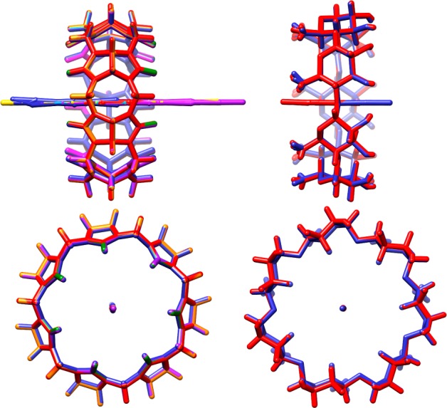
Time-average structures for the bound state of the host–guest systems presented in Table 2. (Left) Superposition of each CB7-All8 host–guest system. (Right) Superposition of the βCD-Hex_Temp host–guest system at 300 K in both the primary and secondary orientations.

One potential concern with the present single-box direct approach to computing binding enthalpies is that the guest in its pulled-free state might not really be far enough from the host to be considered noninteracting. We addressed this issue by comparing the present results with those from our prior multi-box direct enthalpy calculations,²⁰ in which the noninteracting state is represented by two separate simulations, one for the host and one for the guest, so that host–guest interaction is eliminated in the unbound state. Figure S4 confirms that the present single-box results are indistinguishable from those of the multi-box approach and thus supports our choice of separation distance as being adequate. Additionally, to confirm that the calculated thermodynamic values did not depend on our specific choice of atoms for the restraint scheme, we performed an additional set of calculations, labeled βCD-Hex_Alt, in which an alternate set of atoms was chosen as the restraint points. The results showed excellent agreement with the βCD-Hex_Temp values (see Table S2).

3.2. Direct and van’t Hoff Binding Enthalpy

The binding enthalpy can be computed directly, i.e., from potential energies, or via the van’t Hoff equation, which exploits the temperature dependence of the binding free energy.³⁵ Since we can now calculate both binding free energies and direct binding enthalpies at high precision, we have the opportunity to test for self-consistency by comparing binding enthalpies obtained directly with those obtained from binding free energy calculations at several temperatures. We explored this in the CB7-B2_Temp and βCD-Hex_Temp simulation sets, wherein binding free energies were calculated at seven and five temperatures, respectively, centered at 300 K (Figure 7, top). The consistency between the direct and van’t Hoff binding enthalpy results, shown in Table 3, supports the validity of both the binding free energies and the direct enthalpies. It is also of interest that convergence plots of the binding enthalpies from both approaches (Figure 7, bottom) show that the van’t Hoff approach is much more sensitive to extending the simulation time and hence is significantly more difficult to converge than the direct approach. Also, for both systems tested, the final statistical uncertainty is much larger for the van’t Hoff approach (Table 3) and comes at a much higher computational cost in terms of simulation time (Tables S1 and S2).

Table 3. Thermodynamic Binding Values for Validation and Internal Consistency^a.

		ΔGbind at 300 K		direct ΔHbind at 300 K		van’t Hoff ΔHbind at 300 K
simulation set	host, guest	TI/Block	MBAR/StIn	Block	StIn	TI/Block	MBAR/StIn
CB7-All8	CB7, B2	–21.25 ± 0.22	–21.22 ± 0.26	–21.59 ± 0.41	–21.59 ± 0.36
CB7-B2Temp	CB7, B2	–21.32 ± 0.13	–21.36 ± 0.07	–21.65 ± 0.47	–21.65 ± 0.28	–20.78 ± 1.09	–20.66 ± 0.67
CB7-B2HMR	CB7, B2	–21.27 ± 0.41	–21.33 ± 0.12	–21.78 ± 0.44	–21.78 ± 0.31
βCD-HexTemp	βCD, Hex	–3.86 ± 0.17	–3.86 ± 0.09	–1.13 ± 0.66	–1.11 ± 0.41	–0.81 ± 1.72	–0.38 ± 0.89
βCD-HexHMR	βCD, Hex	–3.98 ± 0.21	–3.92 ± 0.09	–0.27 ± 0.64	–0.26 ± 0.39
K-ClTemp	K, Cl	–1.94 ± 0.06	–1.94 ± 0.04	3.68 ± 0.28	3.68 ± 0.23	3.35 ± 0.55	3.58 ± 0.42
K-ClSimple	K, Cl	–1.92 ± 0.14	–1.86 ± 0.10	3.45 ± 0.39	3.45 ± 0.35

^aUncertainty values are 95% CI.

Careful inspection of Table 3 shows that the uncertainty values produced by the blocking method are consistently larger than those from the StIn method. Although our automated implementation of the blocking method is expected to produce slightly larger values than an investigator-performed analysis in which the SEM would be assigned based on a plateau in the SEM as a function of block size, the large difference between the two uncertainty estimates was surprising. This difference could lead to alternate interpretations of the data. For example, when comparing the direct and van’t Hoff binding enthalpies of CB7-B2_Temp, a two-sample t-test for equal means (α = 0.05) would not indicate a significant difference based on the blocking uncertainty values, but it would indicate a significant difference when using the StIn uncertainties. This concern led us to develop a toy model that would allow an even more precise validation of our computational calorimetry methods (see Section 3.3) and a deeper investigation into the uncertainty estimation procedures (see Section 3.5).

3.3. Modified Ion-Pair Test Case

Although the agreement between the direct and van’t Hoff binding enthalpies for the two host–guest systems was strongly encouraging, we wanted to test the comparison to even finer precision in order to detect any potential subtle pathologies. Using a modified K-Cl ion pair, which was tuned to exhibit favorable binding during simulation, we performed several further simulation studies to validate the present approach, as follows.

First, we established that the use of noninteracting anchor particles to align the pulling coordinate did not influence the results. The K-Cl_Simple simulation set, which used a single distance restraint in a large water box, produced binding values statistically indistinguishable from the anchor particle aligned K-Cl_Temp simulation set (see Table 3 for results, and see Figure S2 for the anchor particle approach with ions). Additionally, comparison between the K-Cl_Simple and K-Cl_Temp results suggests that use of a smaller rectangular simulation box aligned to the pulling axis does not introduce error into the binding results (Table 3). The binding free energies and direct enthalpies showed excellent agreement to high precision, with confidence intervals of less than 0.15 and 0.40 kcal/mol, respectively. Our modified K-Cl system could be considered particularly challenging due to the rather large charges that we placed on the ions (±1.3). Thus, it is reassuring that the optimized rectangular box (with alignment via anchor particles) did not incorrectly treat the electrostatics of the system.

Finally, we also observed excellent agreement between the direct and van’t Hoff binding enthalpy for this simple test case (Table 3). The small uncertainties in the van’t Hoff binding enthalpies, relative to those for the full host–guest systems, can be attributed to the better behaved temperature dependence of the binding free energy (Figure S5, top), and the convergence behavior of both binding enthalpy methods is correspondingly smooth (Figure S5, bottom).

Interestingly, we noticed that, although the MBAR/StIn uncertainties are consistently smaller than the TI/blocking uncertainties for the K-Cl data, the ratio between the two values is smaller than the ratio observed for the host–guest values (Table 3). Although a slight overestimation of the error is expected by our implementation of the blocking method, the variability of the ratio between the two uncertainty estimates suggests the difference might be influenced by the nature of the system being simulated. Here, the simplicity of the K-Cl systems possibly minimizes the apparent difference in the uncertainty.

Taken together, the results of the K-Cl simulations strongly suggest that the theory and implementation of the APR computational calorimetry framework is valid and numerically sound. As a consequence, it seems likely that the modest deviations between the direct and van’t Hoff binding enthalpies for the host–guest systems arise from statistical, rather than methodological, error. Curiously, however, there is still a systematic tendency for the blocking estimate of error to exceed the StIn estimate. We investigate this further in a subsequent section (see Section 3.5).

3.4. Accelerating Computational Calorimetry with Hydrogen Mass Repartitioning

The HMR technique is appealing because it allows one to double the simulation time for a given elapsed wall-clock time, by going from a 2 fs to a 4 fs MD time step without inducing numerical instabilities.³⁶ It should be noted that, because we are working within the classical approximation of statistical thermodynamics, the quantities that we aim to compute are independent of the atomic masses. Therefore, any error introduced by HMR would derive from changes in the numerical properties of the simulations. In particular, increasing the time step can increase error by increasing the mean spatial excursion the atoms make in one time step; conversely, increasing the masses of the fastest atoms, i.e., the hydrogens, reduces their mean velocities and hence their mean excursions, for a given temperature, and thus compensates, at least partially, for the increased time step. The net effect could be to influence the values that the computed quantities approach, in the limit of a long simulation. In addition, changing the masses and time step influences the dynamics of the simulations³⁸ and hence can influence the rate of convergence. The net effect of HMR on accuracy and precision is hard to predict.

Therefore, we carried out an empirical evaluation of the feasibility of speeding thermodynamic calculations, while maintaining reliable results, by performing several binding free energy and binding enthalpy calculations with HMR and a 4 fs time step. The results for the CB7-B2_HMR and βCD-Hex_HMR simulations sets, given in Table 3, indicate generally excellent agreement between the standard approach and HMR. (We did not carry out van’t Hoff binding enthalpy measurements, given the excellent agreement between HMR and the traditional approach for the free energy calculations at 300 K.) The one potential outlier is the comparison of the direct binding enthalpy for βCD-Hex. Although a t-test (α = 0.05) would not indicate a significant difference between the binding enthalpy means for βCD-Hex_Temp and βCD-Hex_HMR when using blocking uncertainties, the StIn uncertainties are smaller and thus indicate that the difference in the means is potentially significant. In the following section, we investigate this difference further, show that the difference is due to random statistical chance, and offer evidence that the StIn uncertainty estimate can sometimes be deceptively small.

As noted by others,³⁶ the speedup from HMR does not always double the effective sampling rate due to alterations in the viscosity of the system. Possible evidence of this effect can be found in our data. For example, with a traditional 2 fs time step, the blocking uncertainty values in the βCD-Hex_Temp direct binding enthalpy for the primary and secondary guest orientations are 0.56 and 0.52 kcal/mol, respectively (Table S2). With HMR and the same simulation time (ns), and double the number of data points due to reducing the interval between data writing by one-half, the blocking uncertainty increases to 0.60 and 0.64 kcal/mol. (Note, however, that the real time expenditure of GPU hours for HMR was roughly 60% of the traditional approach.) This suggests that HMR may influence the effective sampling rate to some degree, but the result could be due to random chance and thus requires further study to make a definitive conclusion. The same trend is not always evident for similar comparisons elsewhere in our data, possibly because the effect is clouded by our evolving methodology for performing the calculations.

Overall, HMR does seem to offer an effective increase in sampling rate without impacting the fidelity of the calculations, but the effective speed up is not always straightforward to determine.

3.5. Comparison of Uncertainty Measures

As discussed in prior subsections, the two approaches we employ to estimate uncertainty, blocking analysis and StIn, can give very similar estimates for the SEM of a time-averaged quantity obtained from MD simulations, especially for simple systems, such as our K-Cl model (Figure 8, top). However, we noticed that the two approaches can disagree substantially for more complicated systems, such as a host–guest complex (Figure 8, bottom). In the latter case, it appears that the StIn approach may register relatively fast fluctuations while missing the consequences of slower processes, leading to underestimates of the SEM.

Figure 8.

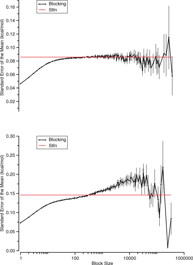
Typical blocking curves for the potential energy of the bound state for a K-Cl_Temp simulation (top) and a βCD-Hex_Temp simulation (bottom). Error bars are an estimate of the uncertainty in the SEM; see Flyvbjerg et al.⁴⁰ for further details. The SEM predicted by the statistical inefficiency method (StIn) is indicated with a red line.

In the present context, it was of particular concern that comparison of the direct binding enthalpy values obtained from the βCD-Hex_Temp and βCD-Hex_HMR simulation sets (Table 3) shows a discrepancy in the uncertainty values, which could impact the conclusions drawn about the difference in the means, as noted above. We traced the primary difference between the two binding enthalpy values to a single source: the average potential energy value of the bound state in the secondary orientation. There were no structural indications to suggest that the sampling had been biased, so we reran one replicate of this particular simulation for each simulation set. The mean of the βCD-Hex_HMR replicate was less than 0.1 kcal/mol from the original value, whereas the βCD-Hex_Temp replicate differed from the original by 0.6 kcal/mol, and four additional βCD-Hex_Temp replicates differed from the original by 0.3–0.7 kcal/mol. Thus, it appeared that the original βCD-Hex_Temp mean value was simply a low probability, but reasonable, value from the tail of the expected normal distribution of mean values. Using the βCD-Hex_Temp replicates, we compared the observed SEM value with the average blocking SEM value and average StIn SEM value. The observed SEM for the six calculations (i.e., the standard deviation of the means for the one original value and five additional replicates) was 0.24 kcal/mol, the average blocking SEM was 0.20 kcal/mol, and the average StIn SEM was 0.14 kcal/mol. The results show closer agreement between the blocking SEM and the observed SEM and suggest that there is no statistical difference between the βCD-Hex_Temp and βCD-Hex_HMR direct binding enthalpy values (according to the t-test), whereas the StIn uncertainty values would indicate a statistical difference.

In order to test more systematically whether the StIn method underestimates the uncertainty in some cases, we developed a Python script (Figure S6) that generates artificial simulation data containing a short-correlation/large-variance process, mixed with several long-correlation/small-variance processes. The resulting time-series data (Figure S7, top) yield blocking analysis graphs (Figure S7, bottom) similar to those from real host–guest data (Figure 8, bottom). By using this method to generate 500 distinct, artificial simulation data sets, we were able to calculate the actual SEM as a function of simulation time and use this to test the ability of the blocking and StIn methods to estimate this observed SEM. In order to generate a summary comparison, we averaged the results from blocking analysis and StIn over the same 500 artificial time series (Figure 9). Early in these runs (<10% of the simulation length), both SEM estimators underestimate the observed SEM. However, for the remainder of the data collection, the blocking method closely tracks (and slightly overestimates by 10–15%) the observed SEM, whereas the StIn method underestimates the SEM by roughly 50%.

Figure 9.

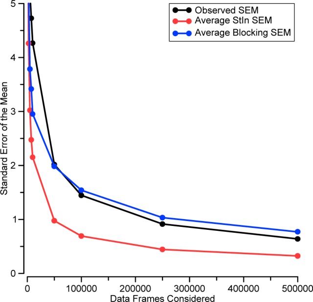
Comparison of the observed SEM (black) with the average StIn SEM (red) and average blocking SEM (blue) for a data set consisting of 500 artificial simulations, each containing 500 000 correlated data points. The artificial simulations contain similar correlation patterns to those observed for real host–guest data (compare Figure 8, bottom, with Figure S7).

A possible explanation for the underestimate by the StIn method can be traced to its approach for computing the integrated correlation time. As detailed previously,³⁹ the tail of the correlation function is generally dominated by noise, which, if included in the integration, tends to make the computed correlation time inaccurate. Following prior practice,³⁹ we addressed this issue by truncating the correlation function when it first crosses zero. To check whether this approach misses useful long-range correlation signals, we performed several tests on the artificial data sets in which the correlation function was not truncated. In each case, however, the estimated uncertainty was even smaller than that obtained with the truncation approach, which itself underestimated the observed uncertainty. Therefore, regardless of whether or not truncation is used, the StIn method appears to be unreliable for the data sets that we studied in this work. We suspect that better reliability of the blocking method can be attributed to two features: (1) the blocking method seems to be sensitive to long-correlation/small-variance signals even when they are obscured by short-correlation/large-variance signals, whereas the StIn method seems to recognize only the latter in the same situation; (2) our automated implementation does not search for a plateau, as in the canonical approach, but reports the largest estimated SEM from the entire blocking curve. The second feature is likely responsible for occasional overestimation of the SEM, but it seems to be the simplest and most conservative method for automation.

4. Discussion

4.1. Computational Calorimetry

Examples of binding affinity calculations are numerous in the literature since they are typically the most sought after value in lead optimization studies. Our computational calorimetry approach provides additional insight simply by extending the end point simulation windows of the APR binding free energy calculation and extracting the binding enthalpy from the difference in mean potential energies. As detailed previously,²⁰ binding enthalpies obtained by the direct method may also be easily decomposed to provide information on the force field terms and/or structural elements that drive binding. As a larger set of host–guest analyses is collected, a more detailed understanding of the role each chemical moiety plays can be established.

Comparison of the calculated and experimental binding free energies, enthalpies, and entropies shows good correlations but large systematic deviations. Given the correlations, one might wonder whether the systematic deviations should be regarded as problematic since, at least in the field of computational ligand design, predicting a correct ranking of ligand affinities is nearly as useful as predicting absolute affinities. However, it is difficult to escape the conclusion that errors of up to ∼10 kcal/mol point to significant problems with the force field that require corrective action, especially given the high precision of the results. Moreover, the types of errors observed here could generate serious practical problems in the more complex setting of protein–ligand binding. In particular, there is no reason to expect that chemically varied ligand moieties interacting with varied subpockets of a protein binding site will be uniformly scaled by whatever factor is generating the systematic bias seen here. As a consequence, there is no assurance of obtaining a good correlation with experiment in such complex systems. Moreover, despite their simplicity, the host–guest systems studied in this work share key attributes of protein–ligand systems, including deep binding cavities with the potential to generate structured water, steric barriers to entry and exit, conformational fluctuations with long time scale correlations, and multiple binding poses. We would argue, therefore, that careful force field optimization to improve the agreement of absolute binding thermodynamics for host–guest systems, in combination with more traditional target data, is a useful path to improve the reliability of protein–ligand modeling for drug discovery.

4.2. Self-consistent Calculations of Binding Thermodynamics

The demonstration of good agreement between the direct and van’t Hoff binding enthalpies for host–guest systems, and of even greater precision for the ion model systems, offers more than a consistency check. Given that robust agreement between the direct and van’t Hoff methods has seemed to be elusive for not only computational investigations¹⁸ but also experimental studies,⁶⁹ there is value in a clear demonstration that rigorous consistency can, in fact, be achieved. Second, consistency between the direct and van’t Hoff binding enthalpy calculations arguably provides strong support for the validity of the binding free energy method employed. This suggests that, as an alternative to assessing error by performing multiple free energy simulations which close a thermodynamic cycle, as is frequently done for alchemical transformations,⁷⁰ one could instead compare direct and van’t Hoff binding enthalpies along a single path. Whether this approach is advantageous will depend on the specifics of the system and the free energy calculation.

The present study also sheds light on the relative merits of the direct versus van’t Hoff binding enthalpy methods. Our data clearly indicate that, for small host–guest systems, the direct binding enthalpy requires less net simulation time to reach a given level of statistical uncertainty. In addition, the direct approach is far simpler to implement than the van’t Hoff approach, at least when the system does not have multiple noninterconverting configurations. The van’t Hoff approach may still be numerically favorable for larger systems, where the potential energy fluctuations are so large that reducing the uncertainty of the mean to a useful level requires extremely long simulations. On the other hand, the challenge of achieving binding free energies that are sufficiently tightly converged to yield meaningful temperature derivatives is not trivial; and the mere technical simplicity of the direct enthalpy approach, which does not require a pathway or lambda windows, is itself a powerful argument in its favor.

4.3. Automation, Sampling, and Timing

With over 438 μs of total sampling across 4434 independent simulations, automation in nearly every aspect of this project was necessary. This included generating the initial coordinates for each simulation along the APR path, solvating the systems with precisely the desired number of water molecules (a feature that is not currently available in AMBER’s LEaP program), determining the correct target values for restraints, and writing all of the input files necessary to perform the simulations. Additionally, our heterogeneous set of computational resources (desktop machines, local clusters, and national clusters) motivated us to develop execution/queuing scripts that simultaneously optimized usage of each resource while maintaining compatibility with the generalized input scripts. Of particular importance was implementation of an automated scheme to determine whether an individual free energy simulation window had reached a predetermined uncertainty threshold in the force uncertainty. Our initial simulation set (CB7-B2_Temp) did not use this feature and, because all windows used the same amount of sampling time, likely oversampled many of the easy-to-converge windows near the pulled-free state. Implementation of our adaptive scheme, which involved iteratively running a short 5 ns simulation followed by checking the uncertainty value of the mean force, improved the sampling efficiency of our other simulation sets. We also note here that the free energy simulation times listed in Tables S1–S3 all include the entire direct binding enthalpy simulations in which the two end point simulations were extended to at least 1 μs each. If one were interested in only computing the binding free energy, then this extra sampling at the end points would not be required, so the aggregate simulation time for a free energy calculation would be lower. Nonetheless, in the cases presented here, removing the additional sampling from the binding free energy simulations would not tilt the balance in favor of the van’t Hoff binding enthalpy approach. For example, Table 1 shows that the extended end point sampling in the CB7-B2_Temp simulation set contributed only, at most, 2.7% of the total sampling time for the van’t Hoff calculations.

This study was feasible in large part to the availability of GPUs, both the commodity and research-grade varieties. Typical simulation speeds for the systems studied here ranged between 150 and 200 ns/day without HMR and up to 350 ns/day with HMR, depending on which generation of hardware was used. With a small cluster of GPUs, both binding enthalpy and free energy values can be computed within a matter of days to highly precise values, with 95% confidence intervals in the range of 0.5 kcal/mol.

As noted in the Methods section, each host studied here posed a distinct challenge to the calculation of well-converged binding free energies. For rigid CB7, the constrictive portal can generate a cork popping problem, whereas flexible βCD can catch on the exiting guest and be pulled into long-lasting distorted conformations. We solved these problems by imposing restraints during the attach phase and lifting them during the release phase, but a variety of enhanced sampling technologies⁷¹⁻⁸⁴ might also have been brought to bear. Indeed, given broad current interest in binding free energy calculations, the computational tractability of these host–guest systems, and the fact that each host examined here exemplifies a different type of sampling challenges, these could be valuable test cases for testing and improving enhanced sampling algorithms.

4.4. Directions

Broader use of the methods laid out here should be facilitated by the fact that our implementation of the APR binding free energy method, and the associated direct calculation of binding enthalpy, is naturally suited to run with nearly all simulation packages that support restraints. No specialized code is required. Automation of the simulation setup still remains a challenge, as it is difficult to foresee a generalized approach for determining the ideal pulling pathway and implementing it with an appropriate restraint setup. However, in most cases, automation for a given host or protein will require setup only for an initial guest or ligand, which can then be used as a template for subsequent compounds.

As noted above, we expect a primary application of computational calorimetry to be force field validation and development. In anticipation of this, we are currently generating a larger data set of calculated host–guest binding values, with multiple force field and water model variants. We anticipate that this approach will be informative since most force fields are not optimized against experimental binding data, even though the calculation of binding affinities, in the context of computer-aided drug design, is one of their most important and prevalent uses. Moreover, the fact that a relatively advanced force field can yield serious errors in binding thermodynamics, as clearly demonstrated here, means that the experimental data traditionally used to adjust force field parameters, such as the hydration free energies of small molecules and the properties of neat liquids, do not suffice when one’s goal is to compute the thermodynamics of noncovalent association. We anticipate that the use of binding data as a force field optimization target, in combination with more traditional targets such as ab initio quantum data, neat liquid properties, and hydration free energies, will be a powerful new tool to improved simulation accuracy.

5. Appendix

The uncertainties in the values obtained directly from simulation (such as mean potential energies and mean forces) are propagated into the thermodynamic values we report. Our approach to this propagation is described below.

5.1. Uncertainty in Thermodynamic Integration Work

We use N_i samples to evaluate the uncertainty of the work terms that yield the binding free energy. For each sample, i, we draw a value of the force in every simulation window from a Gaussian distribution whose average is the mean force and whose standard deviation is the SEM of the mean force (see Section 2.4). We then compute a spline function across the windows, F_i^spl(λ_p,λ_c), and integrate the spline to obtain the ith values of the work. Note that although the scaling factor for the pose restraints and the conformational restraints could be varied independently we scale them simultaneously during the attachment phase. The mean and SEM of the work are computed from the N_i iterations of this procedure. The value of N_i was set to a value, here 10 000, at which added samples did not generate changes in the results to within the precision desired. For the attachment phase:

A1

A2

A3

For the pulling phase, the equilibrium length of the host-guest distance restraint, x_0,1^p is varied, and the spline is fit over discrete windows of this variable:

A4

A5

A6

For releasing conformational restraints

A7

A8

A9

Note that the release of guest translational and rotational restraints is performed analytically and therefore is not associated with a statistical uncertainty.

5.2. Uncertainty in MBAR Work

As noted earlier, we couple the StIn uncertainty approach with the MBAR free energy calculations. The StIn value is calculated for the restraint potential energy time series at each simulation window along the free energy path. The data series is then subsampled according to the StIn value, as previously described,³⁹ and the putatively uncorrelated data points are passed to the MBAR algorithm. The estimated work to move between states, as well as an estimate of the uncertainty, is obtained directly from the MBAR analysis.⁵⁵ Although a single MBAR calculation could be performed for the entire APR pathway, for consistency with the TI approach, we calculated a mean work and SEM for each APR phase.

5.3. Uncertainty in Binding Free Energy

The binding free energy is found by summing the APR work terms, as in eq 1:

A10

Because variances are additive, the SEM uncertainties add in quadrature:

A11

Note that this assumes the variances are not correlated, which is valid for our data given that each simulation window is independent. The work of releasing the guest to standard concentration (W_release-std) does not contribute any uncertainty because it is an analytical calculation.

In cases where multiple distinct binding poses are possible, the combined binding free energy mean and SEM are computed as follows:

A12

A13

Here, N_i is the number of evaluations (we used 1 000 000), N_b is the number of poses (βCD with hexanoate has two), and ΔG_i,j is a random binding free energy selected from a normal distribution defined by the mean and SEM of the value for jth pose and included in the ith evaluation of the equation.

5.4. Uncertainty in Direct Binding Enthalpy

The mean and uncertainty in the direct binding enthalpy calculation is straightforward. The mean is simply the difference between the means of the bound and unbound potential energies.

A14

The uncertainty of the mean is obtained by adding in quadrature the uncertainties of the individual values:

A15

The combined binding enthalpy for multiple poses is determined in a similar fashion to the free energy except that the form of the equation requires random sampling of both the enthalpy and free energy for each pose. The number of evaluations, N_i, and number of poses, N_b, was the same.

A16

A17

5.5. Uncertainty in van’t Hoff Binding Enthalpy

The mean and SEM of the van’t Hoff binding enthalpy were calculated from N_i iterations (we used 100 000) of fitting to eq 14, which we denote ΔH_i^nonlim:

A18

A19

Supporting Information Available

The Supporting Information is available free of charge on the ACS Publications website at DOI: 10.1021/acs.jctc.5b00405.

• Restraint details for each simulation set; detailed force equations; tables with data for all thermodynamic calculations in this work; detailed attach–pull–release restraint figures; snapshot of CB7 with conformational restraints; comparison of one-box versus multi-box binding enthalpies; plots of K-Cl_Temp van’t Hoff binding enthalpy data; Python code for generation of artificially correlated data sets; comparison of uncertainty measurements for the artificially correlated data (PDF)

• A compressed archive file with Mol2 and parameter files necessary for building the hosts and guests in this work (ZIP)

This work used computational resources from both the Triton Shared Computing Cluster at UCSD and the Extreme Science and Engineering Discovery Environment (XSEDE), which is supported by National Science Foundation grant no. ACI-1053575. M.K.G. acknowledges funding from National Institute of General Medical Sciences (GM61300).

The authors declare the following competing financial interest(s): M.K.G. has an equity interest in and is a cofounder and scientific advisor of VeraChem LLC.

References

- Lumry R.; Rajender S. Enthalpy–entropy Compensation Phenomena in Water Solutions of Proteins and Small Molecules: A Ubiquitous Properly of Water. Biopolymers 1970, 9 (10), 1125–1227. 10.1002/bip.1970.360091002. [DOI] [PubMed] [Google Scholar]
- Krug R. R.; Hunter W. G.; Grieger R. A. Statistical Interpretation of Enthalpy–entropy Compensation. Nature 1976, 261 (5561), 566–567. 10.1038/261566a0. [DOI] [Google Scholar]
- Sharp K. Entropy-Enthalpy Compensation: Fact or Artifact?. Protein Sci. 2001, 10 (3), 661–667. 10.1110/ps.37801. [DOI] [PMC free article] [PubMed] [Google Scholar]
- Dunitz J. D. Win Some, Lose Some: Enthalpy-Entropy Compensation in Weak Intermolecular Interactions. Chem. Biol. 1995, 2 (11), 709–712. 10.1016/1074-5521(95)90097-7. [DOI] [PubMed] [Google Scholar]
- Olsson T. S. G.; Ladbury J. E.; Pitt W. R.; Williams M. A. Extent of Enthalpy–entropy Compensation in Protein–ligand Interactions. Protein Sci. 2011, 20 (9), 1607–1618. 10.1002/pro.692. [DOI] [PMC free article] [PubMed] [Google Scholar]
- Reynolds C. H.; Holloway M. K. Thermodynamics of Ligand Binding and Efficiency. ACS Med. Chem. Lett. 2011, 2 (6), 433–437. 10.1021/ml200010k. [DOI] [PMC free article] [PubMed] [Google Scholar]
- Fenley A. T.; Muddana H. S.; Gilson M. K. Entropy–Enthalpy Transduction Caused by Conformational Shifts Can Obscure the Forces Driving Protein–ligand Binding. Proc. Natl. Acad. Sci. U. S. A. 2012, 109 (49), 20006–20011. 10.1073/pnas.1213180109. [DOI] [PMC free article] [PubMed] [Google Scholar]
- Chodera J. D.; Mobley D. L. Entropy-Enthalpy Compensation: Role and Ramifications in Biomolecular Ligand Recognition and Design. Annu. Rev. Biophys. 2013, 42 (1), 121–142. 10.1146/annurev-biophys-083012-130318. [DOI] [PMC free article] [PubMed] [Google Scholar]
- Whitesides G. M.; Krishnamurthy V. M. Designing Ligands to Bind Proteins. Q. Rev. Biophys. 2005, 38 (04), 385–395. 10.1017/S0033583506004240. [DOI] [PMC free article] [PubMed] [Google Scholar]
- Velázquez Campoy A.; Freire E. ITC in the Post-Genomic Era···? Priceless. Biophys. Chem. 2005, 115 (2–3), 115–124. 10.1016/j.bpc.2004.12.015. [DOI] [PubMed] [Google Scholar]
- Freire E. Do Enthalpy and Entropy Distinguish First in Class from Best in Class?. Drug Discovery Today 2008, 13 (19–20), 869–874. 10.1016/j.drudis.2008.07.005. [DOI] [PMC free article] [PubMed] [Google Scholar]
- Scott A. D.; Phillips C.; Alex A.; Flocco M.; Bent A.; Randall A.; O’Brien R.; Damian L.; Jones L. H. Thermodynamic Optimisation in Drug Discovery: A Case Study Using Carbonic Anhydrase Inhibitors. ChemMedChem 2009, 4 (12), 1985–1989. 10.1002/cmdc.200900386. [DOI] [PubMed] [Google Scholar]
- Benfield A. P.; Teresk M. G.; Plake H. R.; DeLorbe J. E.; Millspaugh L. E.; Martin S. F. Ligand Preorganization May Be Accompanied by Entropic Penalties in Protein–Ligand Interactions. Angew. Chem., Int. Ed. 2006, 45 (41), 6830–6835. 10.1002/anie.200600844. [DOI] [PubMed] [Google Scholar]
- DeLorbe J. E.; Clements J. H.; Teresk M. G.; Benfield A. P.; Plake H. R.; Millspaugh L. E.; Martin S. F. Thermodynamic and Structural Effects of Conformational Constraints in Protein–Ligand Interactions. Entropic Paradoxy Associated with Ligand Preorganization. J. Am. Chem. Soc. 2009, 131 (46), 16758–16770. 10.1021/ja904698q. [DOI] [PubMed] [Google Scholar]
- Ladbury J. E.; Klebe G.; Freire E. Adding Calorimetric Data to Decision Making in Lead Discovery: A Hot Tip. Nat. Rev. Drug Discovery 2010, 9 (1), 23–27. 10.1038/nrd3054. [DOI] [PubMed] [Google Scholar]
- Levy R. M.; Gallicchio E. Computer Simulations with Explicit Solvent: Recent Progress in the Thermodynamic Decomposition of Free Energies and in Modeling Electrostatic Effects. Annu. Rev. Phys. Chem. 1998, 49 (1), 531–567. 10.1146/annurev.physchem.49.1.531. [DOI] [PubMed] [Google Scholar]
- Lu N.; Kofke D. A.; Woolf T. B. Staging Is More Important than Perturbation Method for Computation of Enthalpy and Entropy Changes in Complex Systems. J. Phys. Chem. B 2003, 107 (23), 5598–5611. 10.1021/jp027627j. [DOI] [Google Scholar]
- Wyczalkowski M. A.; Vitalis A.; Pappu R. V. New Estimators for Calculating Solvation Entropy and Enthalpy and Comparative Assessments of Their Accuracy and Precision. J. Phys. Chem. B 2010, 114 (24), 8166–8180. 10.1021/jp103050u. [DOI] [PubMed] [Google Scholar]
- Lai B.; Oostenbrink C. Binding Free Energy, Energy and Entropy Calculations Using Simple Model Systems. Theor. Chem. Acc. 2012, 131 (10), 1–13. 10.1007/s00214-012-1272-1. [DOI] [Google Scholar]
- Fenley A. T.; Henriksen N. M.; Muddana H. S.; Gilson M. K. Bridging Calorimetry and Simulation through Precise Calculations of Cucurbituril–Guest Binding Enthalpies. J. Chem. Theory Comput. 2014, 10 (9), 4069–4078. 10.1021/ct5004109. [DOI] [PMC free article] [PubMed] [Google Scholar]
- Rekharsky M. V.; Mayhew M. P.; Goldberg R. N.; Ross P. D.; Yamashoji Y.; Inoue Y. Thermodynamic and Nuclear Magnetic Resonance Study of the Reactions of A- and B-Cyclodextrin with Acids, Aliphatic Amines, and Cyclic Alcohols. J. Phys. Chem. B 1997, 101 (1), 87–100. 10.1021/jp962715n. [DOI] [Google Scholar]
- Rekharsky M. V.; Inoue Y. Complexation Thermodynamics of Cyclodextrins. Chem. Rev. 1998, 98 (5), 1875–1918. 10.1021/cr970015o. [DOI] [PubMed] [Google Scholar]
- Rekharsky M.; Inoue Y. Chiral Recognition Thermodynamics of B-Cyclodextrin: The Thermodynamic Origin of Enantioselectivity and the Enthalpy–Entropy Compensation Effect. J. Am. Chem. Soc. 2000, 122 (18), 4418–4435. 10.1021/ja9921118. [DOI] [Google Scholar]
- Kim H.-J.; Jeon W. S.; Ko Y. H.; Kim K. Inclusion of Methylviologen in cucurbit[7]uril. Proc. Natl. Acad. Sci. U. S. A. 2002, 99 (8), 5007–5011. 10.1073/pnas.062656699. [DOI] [PMC free article] [PubMed] [Google Scholar]
- Liu S.; Ruspic C.; Mukhopadhyay P.; Chakrabarti S.; Zavalij P. Y.; Isaacs L. The Cucurbit[n]uril Family: Prime Components for Self-Sorting Systems. J. Am. Chem. Soc. 2005, 127 (45), 15959–15967. 10.1021/ja055013x. [DOI] [PubMed] [Google Scholar]
- Logsdon L. A.; Schardon C. L.; Ramalingam V.; Kwee S. K.; Urbach A. R. Nanomolar Binding of Peptides Containing Noncanonical Amino Acids by a Synthetic Receptor. J. Am. Chem. Soc. 2011, 133 (42), 17087–17092. 10.1021/ja207825y. [DOI] [PubMed] [Google Scholar]
- Moghaddam S.; Yang C.; Rekharsky M.; Ko Y. H.; Kim K.; Inoue Y.; Gilson M. K. New Ultrahigh Affinity Host–Guest Complexes of Cucurbit[7]uril with Bicyclo[2.2.2]octane and Adamantane Guests: Thermodynamic Analysis and Evaluation of M2 Affinity Calculations. J. Am. Chem. Soc. 2011, 133 (10), 3570–3581. 10.1021/ja109904u. [DOI] [PMC free article] [PubMed] [Google Scholar]
- Wang Y.; King J. R.; Wu P.; Pelzman D. L.; Beratan D. N.; Toone E. J. Enthalpic Signature of Methonium Desolvation Revealed in a Synthetic Host–Guest System Based on Cucurbit[7]uril. J. Am. Chem. Soc. 2013, 135 (16), 6084–6091. 10.1021/ja311327v. [DOI] [PubMed] [Google Scholar]
- Miskolczy Z.; Harangozó J. G.; Biczók L.; Wintgens V.; Lorthioir C.; Amiel C. Effect of Torsional Isomerization and Inclusion Complex Formation with cucurbit[7]uril on the Fluorescence of 6-Methoxy-1-Methylquinolinium. Photochem. Photobiol. Sci. 2014, 13 (3), 499–508. 10.1039/C3PP50307K. [DOI] [PubMed] [Google Scholar]
- Lee J. W.; Lee H. H. L.; Ko Y. H.; Kim K.; Kim H. I. Deciphering the Specific High-Affinity Binding of Cucurbit[7]uril to Amino Acids in Water. J. Phys. Chem. B 2015, 119 (13), 4628–4636. 10.1021/acs.jpcb.5b00743. [DOI] [PubMed] [Google Scholar]
- Salomon-Ferrer R.; Götz A. W.; Poole D.; Le Grand S.; Walker R. C. Routine Microsecond Molecular Dynamics Simulations with AMBER on GPUs. 2. Explicit Solvent Particle Mesh Ewald. J. Chem. Theory Comput. 2013, 9 (9), 3878–3888. 10.1021/ct400314y. [DOI] [PubMed] [Google Scholar]
- Sellner B.; Zifferer G.; Kornherr A.; Krois D.; Brinker U. H. Molecular Dynamics Simulations of B-Cyclodextrin–Aziadamantane Complexes in Water. J. Phys. Chem. B 2008, 112 (3), 710–714. 10.1021/jp075493+. [DOI] [PubMed] [Google Scholar]
- Roy A.; Hua D. P.; Ward J. M.; Post C. B. Relative Binding Enthalpies from Molecular Dynamics Simulations Using a Direct Method. J. Chem. Theory Comput. 2014, 10 (7), 2759–2768. 10.1021/ct500200n. [DOI] [PMC free article] [PubMed] [Google Scholar]
- Henriksen N. M.; Hayatshahi H. S.; Davis D. R.; Cheatham T. E. Structural and Energetic Analysis of 2-Aminobenzimidazole Inhibitors in Complex with the Hepatitis C Virus IRES RNA Using Molecular Dynamics Simulations. J. Chem. Inf. Model. 2014, 54 (6), 1758–1772. 10.1021/ci500132c. [DOI] [PMC free article] [PubMed] [Google Scholar]
- LiCata V. J.; Liu C.-C. Analysis of Free Energy versus Temperature Curves in Protein Folding and Macromolecular Interactions. Methods Enzymol. 2011, 488, 219–238. 10.1016/B978-0-12-381268-1.00009-4. [DOI] [PubMed] [Google Scholar]
- Feenstra K. A.; Hess B.; Berendsen H. J. C. Improving Efficiency of Large Time-Scale Molecular Dynamics Simulations of Hydrogen-Rich Systems. J. Comput. Chem. 1999, 20 (8), 786–798. 10.1002/(SICI)1096-987X(199906)20:8<786::AID-JCC5>3.3.CO;2-2. [DOI] [PubMed] [Google Scholar]
- Harvey M. J.; Giupponi G.; Fabritiis G. D. ACEMD: Accelerating Biomolecular Dynamics in the Microsecond Time Scale. J. Chem. Theory Comput. 2009, 5 (6), 1632–1639. 10.1021/ct9000685. [DOI] [PubMed] [Google Scholar]
- Hopkins C. W.; Le Grand S.; Walker R. C.; Roitberg A. E. Long-Time-Step Molecular Dynamics through Hydrogen Mass Repartitioning. J. Chem. Theory Comput. 2015, 11, 1864–1874. 10.1021/ct5010406. [DOI] [PubMed] [Google Scholar]
- Chodera J. D.; Swope W. C.; Pitera J. W.; Seok C.; Dill K. A. Use of the Weighted Histogram Analysis Method for the Analysis of Simulated and Parallel Tempering Simulations. J. Chem. Theory Comput. 2007, 3 (1), 26–41. 10.1021/ct0502864. [DOI] [PubMed] [Google Scholar]
- Flyvbjerg H.; Petersen H. G. Error Estimates on Averages of Correlated Data. J. Chem. Phys. 1989, 91 (1), 461–466. 10.1063/1.457480. [DOI] [Google Scholar]
- Muddana H. S.; Varnado C. D.; Bielawski C. W.; Urbach A. R.; Isaacs L.; Geballe M. T.; Gilson M. K. Blind Prediction of Host–guest Binding Affinities: A New SAMPL3 Challenge. J. Comput.-Aided Mol. Des. 2012, 26 (5), 475–487. 10.1007/s10822-012-9554-1. [DOI] [PMC free article] [PubMed] [Google Scholar]
- Wang J.; Wang W.; Kollman P. A.; Case D. A. Automatic Atom Type and Bond Type Perception in Molecular Mechanical Calculations. J. Mol. Graphics Modell. 2006, 25 (2), 247–260. 10.1016/j.jmgm.2005.12.005. [DOI] [PubMed] [Google Scholar]
- Jakalian A.; Bush B. L.; Jack D. B.; Bayly C. I. Fast, Efficient Generation of High-Quality Atomic Charges. AM1-BCC Model: I. Method. J. Comput. Chem. 2000, 21 (2), 132–146. 10.1002/(SICI)1096-987X(20000130)21:2<132::AID-JCC5>3.0.CO;2-P. [DOI] [PubMed] [Google Scholar]
- Jakalian A.; Jack D. B.; Bayly C. I. Fast, Efficient Generation of High-Quality Atomic Charges. AM1-BCC Model: II. Parameterization and Validation. J. Comput. Chem. 2002, 23 (16), 1623–1641. 10.1002/jcc.10128. [DOI] [PubMed] [Google Scholar]
- Wang J.; Wolf R. M.; Caldwell J. W.; Kollman P. A.; Case D. A. Development and Testing of a General Amber Force Field. J. Comput. Chem. 2004, 25 (9), 1157–1174. 10.1002/jcc.20035. [DOI] [PubMed] [Google Scholar]
- Cézard C.; Trivelli X.; Aubry F.; Djedaïni-Pilard F.; Dupradeau F.-Y. Molecular Dynamics Studies of Native and Substituted Cyclodextrins in Different Media: 1. Charge Derivation and Force Field Performances. Phys. Chem. Chem. Phys. 2011, 13 (33), 15103–15121. 10.1039/c1cp20854c. [DOI] [PubMed] [Google Scholar]
- Bayly C. I.; Cieplak P.; Cornell W.; Kollman P. A. A Well-Behaved Electrostatic Potential Based Method Using Charge Restraints for Deriving Atomic Charges: The RESP Model. J. Phys. Chem. 1993, 97 (40), 10269–10280. 10.1021/j100142a004. [DOI] [Google Scholar]
- Dupradeau F.-Y.; Pigache A.; Zaffran T.; Savineau C.; Lelong R.; Grivel N.; Lelong D.; Rosanski W.; Cieplak P. The R.E.D. Tools: Advances in RESP and ESP Charge Derivation and Force Field Library Building. Phys. Chem. Chem. Phys. 2010, 12 (28), 7821–7839. 10.1039/c0cp00111b. [DOI] [PMC free article] [PubMed] [Google Scholar]
- Vanquelef E.; Simon S.; Marquant G.; Garcia E.; Klimerak G.; Delepine J. C.; Cieplak P.; Dupradeau F.-Y. R.E.D. R.E.D. Server: A Web Service for Deriving RESP and ESP Charges and Building Force Field Libraries for New Molecules and Molecular Fragments. Nucleic Acids Res. 2011, 39, W511–W517. 10.1093/nar/gkr288. [DOI] [PMC free article] [PubMed] [Google Scholar]
- Steinbrecher T.; Latzer J.; Case D. A. Revised AMBER Parameters for Bioorganic Phosphates. J. Chem. Theory Comput. 2012, 8 (11), 4405–4412. 10.1021/ct300613v. [DOI] [PMC free article] [PubMed] [Google Scholar]
- Åqvist J. Ion-Water Interaction Potentials Derived from Free Energy Perturbation Simulations. J. Phys. Chem. 1990, 94 (21), 8021–8024. 10.1021/j100384a009. [DOI] [Google Scholar]
- Dang L. X. Mechanism and Thermodynamics of Ion Selectivity in Aqueous Solutions of 18-Crown-6 Ether: A Molecular Dynamics Study. J. Am. Chem. Soc. 1995, 117 (26), 6954–6960. 10.1021/ja00131a018. [DOI] [Google Scholar]
- Auffinger P.; Cheatham T. E.; Vaiana A. C. Spontaneous Formation of KCl Aggregates in Biomolecular Simulations: A Force Field Issue?. J. Chem. Theory Comput. 2007, 3 (5), 1851–1859. 10.1021/ct700143s. [DOI] [PubMed] [Google Scholar]
- Velez-Vega C.; Gilson M. K. Overcoming Dissipation in the Calculation of Standard Binding Free Energies by Ligand Extraction. J. Comput. Chem. 2013, 34 (27), 2360–2371. 10.1002/jcc.23398. [DOI] [PMC free article] [PubMed] [Google Scholar]
- Shirts M. R.; Chodera J. D. Statistically Optimal Analysis of Samples from Multiple Equilibrium States. J. Chem. Phys. 2008, 129 (12), 124105. 10.1063/1.2978177. [DOI] [PMC free article] [PubMed] [Google Scholar]
- Swope W. C.; Andersen H. C.; Berens P. H.; Wilson K. R. A Computer Simulation Method for the Calculation of Equilibrium Constants for the Formation of Physical Clusters of Molecules: Application to Small Water Clusters. J. Chem. Phys. 1982, 76 (1), 637–649. 10.1063/1.442716. [DOI] [Google Scholar]
- Woo H.-J.; Roux B. Calculation of Absolute Protein–ligand Binding Free Energy from Computer Simulations. Proc. Natl. Acad. Sci. U. S. A. 2005, 102 (19), 6825–6830. 10.1073/pnas.0409005102. [DOI] [PMC free article] [PubMed] [Google Scholar]
- Pettersen E. F.; Goddard T. D.; Huang C. C.; Couch G. S.; Greenblatt D. M.; Meng E. C.; Ferrin T. E. UCSF Chimera—A Visualization System for Exploratory Research and Analysis. J. Comput. Chem. 2004, 25 (13), 1605–1612. 10.1002/jcc.20084. [DOI] [PubMed] [Google Scholar]
- Mobley D. L.; Chodera J. D.; Dill K. A. Confine-and-Release Method: Obtaining Correct Binding Free Energies in the Presence of Protein Conformational Change. J. Chem. Theory Comput. 2007, 3 (4), 1231–1235. 10.1021/ct700032n. [DOI] [PMC free article] [PubMed] [Google Scholar]
- Fenley A. T.; Muddana H. S.; Gilson M. K. Calculation and Visualization of Atomistic Mechanical Stresses in Nanomaterials and Biomolecules. PLoS One 2014, 9 (12), e113119. 10.1371/journal.pone.0113119. [DOI] [PMC free article] [PubMed] [Google Scholar]
- Case D. A.; Babin V.; Berryman J. T.; Betz R. M.; Cai Q.; Cerutti D.S.; Cheatham T. E. III; Darden T. A.; Duke R. E.; Gohlke H.; Goetz A. W.; Gusarov S.; Homeyer N.; Janowski P.; Kaus J.; Kolossváry I.; Kovalenko A.; Lee T. S.; LeGrand S.; Luchko T.; Luo R.; Madej B.; Merz K. M.; Paesani F.; Roe D. R.; Roitberg A.; Sagui C.; Salomen-Ferrer R.; Seabra G.; Simmerling C. L.; Smith W.; Swails J.; Walker R. C.; Wang J.; Wolf R. M.; Wu X.; Kollman P. A.. Amber 14; University of California, San Francisco: San Francisco, CA, 2014.
- Loncharich R. J.; Brooks B. R.; Pastor R. W. Langevin Dynamics of Peptides: The Frictional Dependence of Isomerization Rates of N-Acetylalanyl-N′-Methylamide. Biopolymers 1992, 32 (5), 523–535. 10.1002/bip.360320508. [DOI] [PubMed] [Google Scholar]
- Åqvist J.; Wennerström P.; Nervall M.; Bjelic S.; Brandsdal B. O. Molecular Dynamics Simulations of Water and Biomolecules with a Monte Carlo Constant Pressure Algorithm. Chem. Phys. Lett. 2004, 384 (4–6), 288–294. 10.1016/j.cplett.2003.12.039. [DOI] [Google Scholar]
- Berendsen H. J. C.; Postma J. P. M.; van Gunsteren W. F.; DiNola A.; Haak J. R. Molecular Dynamics with Coupling to an External Bath. J. Chem. Phys. 1984, 81 (8), 3684–3690. 10.1063/1.448118. [DOI] [Google Scholar]
- Darden T.; York D.; Pedersen L. Particle Mesh Ewald: An N·log(N) Method for Ewald Sums in Large Systems. J. Chem. Phys. 1993, 98 (12), 10089–10092. 10.1063/1.464397. [DOI] [Google Scholar]
- Essmann U.; Perera L.; Berkowitz M. L.; Darden T.; Lee H.; Pedersen L. G. A Smooth Particle Mesh Ewald Method. J. Chem. Phys. 1995, 103 (19), 8577–8593. 10.1063/1.470117. [DOI] [Google Scholar]
- Ryckaert J.-P.; Ciccotti G.; Berendsen H. J. C. Numerical Integration of the Cartesian Equations of Motion of a System with Constraints: Molecular Dynamics of N-Alkanes. J. Comput. Phys. 1977, 23 (3), 327–341. 10.1016/0021-9991(77)90098-5. [DOI] [Google Scholar]
- Miyamoto S.; Kollman P. A. Settle: An Analytical Version of the SHAKE and RATTLE Algorithm for Rigid Water Models. J. Comput. Chem. 1992, 13 (8), 952–962. 10.1002/jcc.540130805. [DOI] [Google Scholar]
- Horn J. R.; Russell D.; Lewis E. A.; Murphy K. P. Van’t Hoff and Calorimetric Enthalpies from Isothermal Titration Calorimetry: Are There Significant Discrepancies?†. Biochemistry 2001, 40 (6), 1774–1778. 10.1021/bi002408e. [DOI] [PubMed] [Google Scholar]
- Liu S.; Wu Y.; Lin T.; Abel R.; Redmann J. P.; Summa C. M.; Jaber V. R.; Lim N. M.; Mobley D. L. Lead Optimization Mapper: Automating Free Energy Calculations for Lead Optimization. J. Comput.-Aided Mol. Des. 2013, 27 (9), 755–770. 10.1007/s10822-013-9678-y. [DOI] [PMC free article] [PubMed] [Google Scholar]
- Hamelberg D.; Mongan J.; McCammon J. A. Accelerated Molecular Dynamics: A Promising and Efficient Simulation Method for Biomolecules. J. Chem. Phys. 2004, 120 (24), 11919–11929. 10.1063/1.1755656. [DOI] [PubMed] [Google Scholar]
- Fukunishi H.; Watanabe O.; Takada S. On the Hamiltonian Replica Exchange Method for Efficient Sampling of Biomolecular Systems: Application to Protein Structure Prediction. J. Chem. Phys. 2002, 116 (20), 9058–9067. 10.1063/1.1472510. [DOI] [Google Scholar]
- Nadler W.; Hansmann U. H. E. Generalized Ensemble and Tempering Simulations: A Unified View. Phys. Rev. E 2007, 75 (2), 026109. 10.1103/PhysRevE.75.026109. [DOI] [PubMed] [Google Scholar]
- Nakajima N.; Nakamura H.; Kidera A. Multicanonical Ensemble Generated by Molecular Dynamics Simulation for Enhanced Conformational Sampling of Peptides. J. Phys. Chem. B 1997, 101 (5), 817–824. 10.1021/jp962142e. [DOI] [Google Scholar]
- Elber R.; Karplus M. Enhanced Sampling in Molecular Dynamics: Use of the Time-Dependent Hartree Approximation for a Simulation of Carbon Monoxide Diffusion through Myoglobin. J. Am. Chem. Soc. 1990, 112 (25), 9161–9175. 10.1021/ja00181a020. [DOI] [Google Scholar]
- Wu X.; Damjanovic A.; Brooks B. R.. Efficient and Unbiased Sampling of Biomolecular Systems in the Canonical Ensemble: A Review of Self-Guided Langevin Dynamics. In Advances in Chemical Physics; Rice S. A., Dinner A. R., Eds.; John Wiley & Sons, Inc.: Hoboken, NJ, 2012; pp 255–326. [DOI] [PMC free article] [PubMed] [Google Scholar]
- Okamoto Y. Generalized-Ensemble Algorithms: Enhanced Sampling Techniques for Monte Carlo and Molecular Dynamics Simulations. J. Mol. Graphics Modell. 2004, 22 (5), 425–439. 10.1016/j.jmgm.2003.12.009. [DOI] [PubMed] [Google Scholar]
- Junghans C.; Perez D.; Vogel T. Molecular Dynamics in the Multicanonical Ensemble: Equivalence of Wang–Landau Sampling, Statistical Temperature Molecular Dynamics, and Metadynamics. J. Chem. Theory Comput. 2014, 10 (5), 1843–1847. 10.1021/ct500077d. [DOI] [PubMed] [Google Scholar]
- Barducci A.; Bussi G.; Parrinello M. Well-Tempered Metadynamics: A Smoothly Converging and Tunable Free-Energy Method. Phys. Rev. Lett. 2008, 100 (2), 020603. 10.1103/PhysRevLett.100.020603. [DOI] [PubMed] [Google Scholar]
- Laio A.; Parrinello M. Escaping Free-Energy Minima. Proc. Natl. Acad. Sci. U. S. A. 2002, 99 (20), 12562–12566. 10.1073/pnas.202427399. [DOI] [PMC free article] [PubMed] [Google Scholar]
- Comer J.; Gumbart J. C.; Hénin J.; Lelièvre T.; Pohorille A.; Chipot C. The Adaptive Biasing Force Method: Everything You Always Wanted To Know but Were Afraid To Ask. J. Phys. Chem. B 2015, 119 (3), 1129–1151. 10.1021/jp506633n. [DOI] [PMC free article] [PubMed] [Google Scholar]
- Hansen H. S.; Hünenberger P. H. Using the Local Elevation Method to Construct Optimized Umbrella Sampling Potentials: Calculation of the Relative Free Energies and Interconversion Barriers of Glucopyranose Ring Conformers in Water. J. Comput. Chem. 2010, 31 (1), 1–23. 10.1002/jcc.21253. [DOI] [PubMed] [Google Scholar]
- Sugita Y.; Okamoto Y. Replica-Exchange Molecular Dynamics Method for Protein Folding. Chem. Phys. Lett. 1999, 314 (1–2), 141–151. 10.1016/S0009-2614(99)01123-9. [DOI] [Google Scholar]
- Darve E.; Pohorille A. Calculating Free Energies Using Average Force. J. Chem. Phys. 2001, 115 (20), 9169–9183. 10.1063/1.1410978. [DOI] [Google Scholar]
Associated Data
This section collects any data citations, data availability statements, or supplementary materials included in this article.