Note: Model identification and analysis of bivalent analyte surface plasmon resonance data

Abstract

Surface plasmon resonance (SPR) is a widely used, affinity based, label-free biophysical technique to investigate biomolecular interactions. The extraction of rate constants requires accurate identification of the particular binding model. The bivalent analyte model involves coupled non-linear differential equations. No clear procedure to identify the bivalent analyte mechanism has been established. In this report, we propose a unique signature for the bivalent analyte model. This signature can be used to distinguish the bivalent analyte model from other biphasic models. The proposed method is demonstrated using experimentally measured SPR sensorgrams.

Surface plasmon resonance (SPR) is a well-accepted label-free tool to investigate and analyze biomolecular interactions, including protein-protein,^1–3 protein-DNA,^4–6 and protein-lipid membrane interactions.⁷ Neither the simplest equilibrium SPR data analysis method⁶ nor the single exponential fitting of SPR profiles⁸ can handle biphasic reaction mechanisms. Several reports in order to improve resolution of the SPR system,^9–11 SPR data fitting programs,¹² and an analytical solution based approach for the analysis of several biphasic binding mechanisms that are governed by linear rate equations¹³ have been reported. However, clear procedure to identify the bivalent analyte mechanism has not been established.

In this study, we have explored an approach to identify and analyze the bivalent analyte model that has been used to analyze SPR sensorgrams of a wide range of biomolecular interactions.^14–23 As being demonstrated in our previous study,¹³ measured SPR profiles can often be fitted to different biphasic models with comparable fitting qualities. Therefore, fitting quality alone cannot identify the underlying mechanism. We propose an approach, presented below, that can identify the bivalent model unambiguously. The procedures of data fitting and model identification are illustrated by experimentally measured SPR sensorgrams.

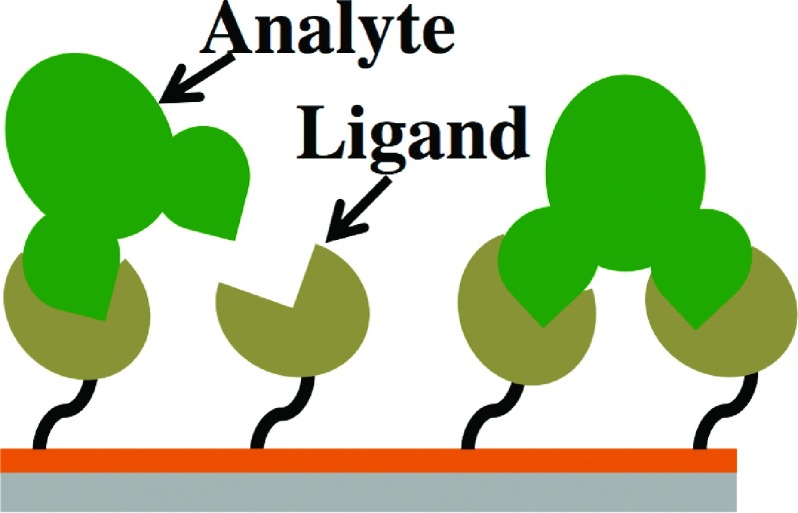
Figure 1 shows the cartoon scheme of the bivalent analyte model, which is represented by the following two-step process:

$${\displaystyle \left[\text{A}\right]+\left[\text{L}\right]\underset{{\mathrm{k}}_{\text{d1}}}{\overset{{\mathrm{k}}_{\text{a1}}}{\rightleftharpoons }}\left[{\text{AL}}_1\right],\left[{\text{AL}}_1\right]+\left[\text{L}\right]\underset{{\mathrm{k}}_{\text{d2}}}{\overset{{\mathrm{k}}_{\text{a2}}}{\rightleftharpoons }}\left[{\text{AL}}_2\right],}$$ (1)

where $\left[\text{A}\right]$ represents bivalent analyte, $\left[\text{L}\right]$ represents ligand, [AL₁] represents analyte-ligand complex with one ligand, and [AL₂] represents analyte-ligand complex with two ligands bound to single analyte. The k_a’s are the association rate constants, and k_d’s are the dissociation rate constants. Let X₁ be [AL₁], and X₂ be [AL₂], the density of free ligand on the sensor chip is thus B₀ − X₁ − 2X₂, with B₀ as the initial ligand concentration. The two-step process of Figure 1 can be represented by the following rate equations:

$${\displaystyle {\dot{\text{X}}}_1=2{\mathrm{k}}_{\text{a1}}\mathrm{C}\left({\mathrm{B}}_0-{\mathrm{X}}_1-2{\mathrm{X}}_2\right)-{\mathrm{k}}_{\text{d1}}{\mathrm{X}}_1-{\dot{\mathrm{X}}}_2,}$$ (2)

$${\displaystyle {\dot{\text{X}}}_2={\mathrm{k}}_{\text{a2}}{\mathrm{X}}_1\left({\mathrm{B}}_0-{\mathrm{X}}_1-2{\mathrm{X}}_2\right)-2{\mathrm{k}}_{\text{d2}}{\mathrm{X}}_2,}$$ (3)

where C is the concentration of analyte.

FIG. 1.

Cartoon scheme for bivalent analyte model.

Strictly speaking, Eq. (3) is only valid when $\left[{\text{AL}}_1\right]$ is freely mobile in the bulk solution. When $\left[{\text{AL}}_1\right]$ is restricted within a layer (reaction layer) on sensor chips, the second association rate constant (k_a2) needs to be replaced by a two dimensional (2D) rate constant, ${\text{k}}_{\text{a2}}^{*}$. As one can see, by comparing Eqs. (2) and (3), that k_a1C and ${\text{k}}_{\text{a2}}^{*}{\text{X}}_1$ must have the same unit of s⁻¹. It is important to understand that the solution of the rate equations (Eqs. (2) and (3)) gives 2D density of ligand-analyte complex, not directly the SPR responses. In the following, for simplicity, we assume that SPR responses are proportional to the combined 2D densities X₁ and X₂.

When rate equations are linear differential equations, it makes the analysis possible to fit SPR sensorgrams directly with solutions of rate equations. For non-linear rate equation, there is no such simplification. Additionally, non-linear differential equations, in general, have no analytical solutions. Therefore, previously proposed method¹³ cannot be directly applied. We rewrite Eqs. (2) and (3) in variables Y = X₁ + X₂ and X₂. The rate equations are in the form of Eqs. (4) and (5),

$${\displaystyle \dot{\text{Y}}=2{\mathrm{k}}_{\text{a1}}\mathrm{C}\left({\mathrm{B}}_{\mathrm{o}}-\mathrm{Y}\right)-{\mathrm{k}}_{\text{d1}}\mathrm{Y}-\left(2{\mathrm{k}}_{\text{a1}}\mathrm{C}-{\mathrm{k}}_{\text{d1}}\right){\mathrm{X}}_2,}$$ (4)

$${\displaystyle \dot{{\text{X}}_2}={\mathrm{k}}_{\text{a2}}^{\ast }\left({\mathrm{X}}_2^2-{\mathrm{Y}}^2\right)+{\mathrm{k}}_{\text{a2}}^{\ast }{\mathrm{B}}_{\mathrm{o}}\mathrm{Y}-\left({\mathrm{k}}_{\text{a2}}^{\ast }{\mathrm{B}}_{\mathrm{o}}-2{\mathrm{k}}_{\text{d2}}\right){\mathrm{X}}_2.}$$ (5)

As expected, Eq. (5) is non-linear, and however, Eq. (4) shows that there exists an “optimal concentration,” ${\text{C}}_{\text{o}}=\frac{{\text{k}}_{\text{d1}}}{2{\text{k}}_{\text{a1}}}$ at which the rate equation for Y is independent of X₂ and, therefore, is a linear differential equation with an analytical solution of single exponential function,

$${\displaystyle \text{Y}\left(\text{t}\right)=\frac{{\text{B}}_0}{2}(1-e^{-\left(2{\text{k}}_{\text{a}1}{\text{C}}_{\text{o}}+{\text{k}}_{\text{d}1}\right)\text{t}})=\frac{{\text{B}}_0}{2}(1-e^{-\left(4{\text{k}}_{\text{a}1}{\text{C}}_{\text{o}}\right)\text{t}}).}$$ (6)

The unknown constant of B₀ in Eq. (6) does not affect the exponent. The exponent, together with C₀, determines k_a1 and k_d1. However, at this “optimal concentration” C_o, the solution $\text{Y}\left(\text{t}\right)$ does not depend on ${\text{k}}_{\text{a}2}^{*}$ or k_d2. Therefore, this “optimal concentration” method will not obtain these two rate constants. At the optimal concentration, the SPR signal does have contributions from both X₁(t) and X₂(t), but the solution contains no information on the relative strength of these two components. In practice, the SPR profiles at different analyte concentration can be fitted individually using single exponential function, and the fitting errors should have a minimum at the “optimal concentration.” The existence of this “optimal concentration” is the unique signature of the bivalent analyte model, thus can be used to distinguish the bivalent-analyte model from other biphasic models that were discussed in our previous study.¹³ It is worthwhile to point out that this signature is discarded in any “global” fitting procedure.

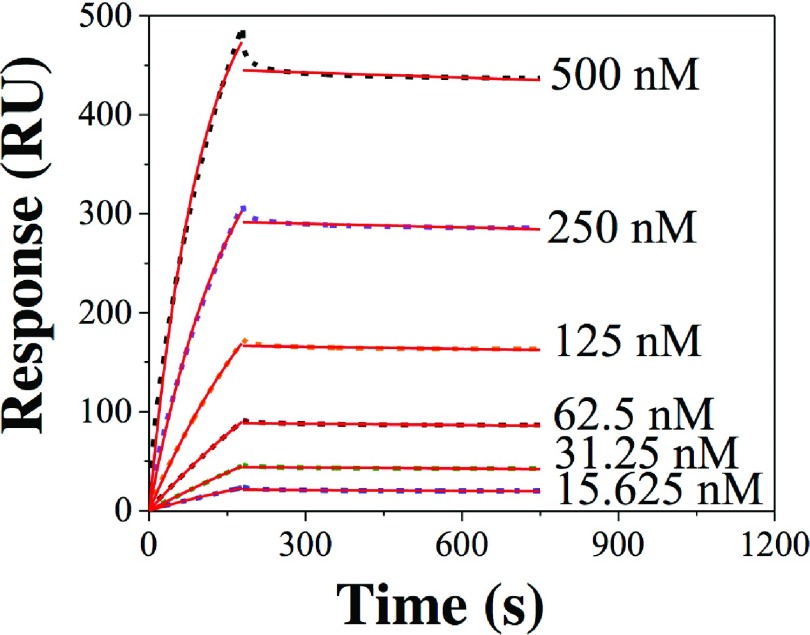
We have demonstrated our theoretical model of identifying the bivalent analyte model using experimentally measured SPR sensorgrams. Biacore T200 instrument was used to record SPR sensorgrams. Sensor chip CM5 was used to immobilize recombinant ezrin proteins onto the sensor surface via standard amine coupling chemistry. Various concentrations (15.625 nM–500 nM) of anti-ezrin monoclonal antibody (ezrinAb) were passed through the ezrin immobilized sensor surface. Figure 2 depicts the SPR sensorgrams for ezrinAb-ezrin binding. As shown in Figure 2, the SPR association profiles did not reach equilibrium state and as a result the simplest equilibrium data analysis method cannot be used. The lowest R² value of fitting of both association and dissociation profiles (Figure 2) was less than 0.75. This indicates that the interaction mechanism is not 1:1. We, therefore, fitted the SPR sensorgrams using following double exponential functions:

$${\displaystyle \text{R}=\text{D}+{\text{Ee}}^{-{\sigma }_{1}t}+{\text{Fe}}^{-{\sigma }_{2}t}\text{(association),}}$$ (7)

$${\displaystyle \text{R}={\text{Ee}}^{-{\gamma }_{1}t}+{\text{Fe}}^{-{\gamma }_{2}t}\text{(dissociation),}}$$ (8)

where D, E, F, σ₁, σ₂, γ₁, and γ₂ are fitting parameters with D = − (E + F). The lowest R² value of fitting of the SPR sensorgram was better than 0.97 (data not shown).

FIG. 2.

SPR sensorgrams for ezrinAb binding to immobilized ezrin. The dashed lines are experimental data and the red continuous lines are fit to single exponential association and dissociation equations.

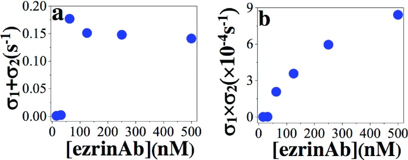
As discussed in our previous report,¹³ a “good” global fitting quality cannot guarantee the correct identification of the underlying mechanism. One should examine the behavior of the exponents (fitting parameters, Eq. (7)) as a function of the analyte concentration. The dependency of the sum of the exponents on ezrinAb concentration as shown in Figure 3(a) shows that underlying mechanism is none of the three models as discussed in detail in our previous report.¹³ In addition, the product of the exponents should be either linear (two-step conformational change model) or quadratic (heterogeneous ligand model and bivalent ligand model) for the biphasic mechanism to be any of the three biphasic mechanisms.¹³ As shown in our previous report, the quadratic dependency must have positive coefficients (coefficients of the quadratic, linear, and constant term in a quadratic equation).¹³ The dependency of the product of the exponents as shown in Figure 3(b) therefore added another validation that the underlying mechanism is not any of the biphasic mechanisms as explained above. Notably, the biphasic models (two-step conformational change model, heterogeneous ligand model, and bivalent ligand model) are governed by coupled system of linear differential equations,¹³ unlike the bivalent analyte model presented in this report.

FIG. 3.

The dependency of (a) the sum of the exponents σ₁ + σ₂ and (b) the product σ₁ × σ₂ on the ezrinAb concentration.

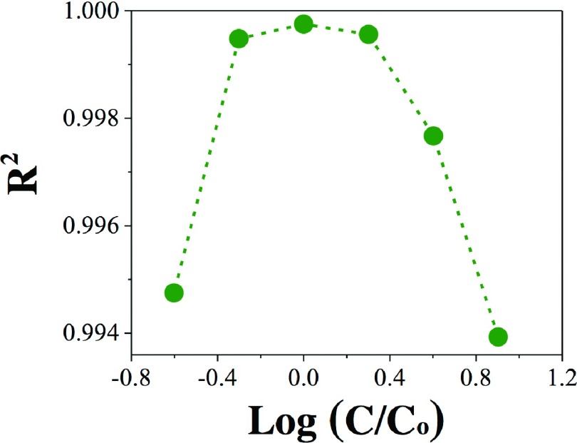
Finally, to correctly identify the underlying biphasic model, we utilized the signature of the bivalent analyte model as explained above. The distribution of R² value obtained by fitting SPR association profiles at different analyte concentrations with single exponential function (Figure 2) is shown in Figure 4.

FIG. 4.

R² value vs. log(C/C_o) for single exponential fitting of SPR association profiles (Figure 2). C is ezrinAb concentration and C_o is the “optimal concentration” (62.5 nM). The symbols are R² values and the dashed lines are guide to eyes.

The distribution of R² value for the experimental data followed exactly the theoretical model as predicted by Eqs. (4) and (6). Therefore, the underlying biphasic mechanism for ezrinAb-ezrin binding should be the bivalent analyte. The monoclonal anti-ezrin antibody is an I_gG₁ type antibody, which has two Fab portions for binding to ezrin. Therefore, the I_gG antibody represents a good model for bivalent analyte. From the fitting of the SPR association profiles (Figure 2), the “optimal concentration” is determined to be 62.5 nM. Once the “optimal concentration” is determined, Eq. (6) can be used to determine the k_a1 and k_d1 and hence the equilibrium dissociation constant (K_D1) of the interaction (${\text{K}}_{\text{D}1}=\frac{{\text{k}}_{\text{d}1}}{{\text{k}}_{\text{a}1}}$) corresponding to the first phase of the interaction. The k_a1, k_d1, and K_D1 values were determined to be 0.74 × 10⁴ M⁻¹ s⁻¹, 0.92 × 10⁻³ s⁻¹, and ∼124 nM, respectively. Our method cannot determine the parameters related to the second phase of the interaction, which are not of any use to determine the K_D2 in terms of molar unit.

In summary, we have presented an identification and analysis of the bivalent analyte model that is applied to a wide range of SPR experiments. The proposed procedure will first locate the “optimal analyte concentration” by fitting the individual SPR profile at different analyte concentrations to the single exponential function. Our method can be of valuable guidance for the SPR users in order to unambiguously identify and analyze the bivalent analyte mechanism. Our procedures of model identification along with the some prior experimental results of the system under study may also provide SPR users a strong support for the identification of the bivalent analyte model.

REFERENCES

- 1.Phizicky E. M. and Fields S., Microbiol. Rev. 59, 94 (1995). [DOI] [PMC free article] [PubMed] [Google Scholar]
- 2.Tiwari P. B., Astudillo L., Miksovska J., Wang X., Li W., Darici Y., and He J., Nanoscale 6, 10255 (2014). 10.1039/C4NR02964J [DOI] [PubMed] [Google Scholar]
- 3.Berggård T., Linse S., and James P., Proteomics 7, 2833 (2007). 10.1002/pmic.200700131 [DOI] [PubMed] [Google Scholar]
- 4.Majka J. and Speck C., in Analytics of Protein–DNA Interactions, edited by Seitz H. (Springer, Berlin Heidelberg, 2007). [Google Scholar]
- 5.Tsoi P. Y. and Yang M., Biosens. Bioelectron. 19, 1209 (2004). 10.1016/j.bios.2003.11.004 [DOI] [PubMed] [Google Scholar]
- 6.Tiwari P. B., Annamalai T., Cheng B., Narula G., Wang X., Tse-Dinh Y.-C., He J., and Darici Y., Biochem. Biophys. Res. Commun. 445, 445 (2014). 10.1016/j.bbrc.2014.02.015 [DOI] [PMC free article] [PubMed] [Google Scholar]
- 7.Wang W., Yang Y., Wang S., Nagaraj V. J., Liu Q., Wu J., and Tao N., Nat. Chem. 4, 846 (2012). 10.1038/nchem.1434 [DOI] [PMC free article] [PubMed] [Google Scholar]
- 8.Tóth A., Kiss E., Herberg F. W., Gergely P., Hartshorne D. J., and Erdödi F., Eur. J. Biochem. 267, 1687 (2000). 10.1046/j.1432-1327.2000.01158.x [DOI] [PubMed] [Google Scholar]
- 9.Filion-Côté S., Roche P. J. R., Foudeh A. M., Tabrizian M., and Kirk A. G., Rev. Sci. Instrum. 85, 093107 (2014). 10.1063/1.4894655 [DOI] [PubMed] [Google Scholar]
- 10.Zhang H. Q., Boussaad S., and Tao N. J., Rev. Sci. Instrum. 74, 150 (2003). 10.1063/1.1523649 [DOI] [Google Scholar]
- 11.Tao N. J., Boussaad S., Huang W. L., Arechabaleta R. A., and D’Agnese J., Rev. Sci. Instrum. 70, 4656 (1999). 10.1063/1.1150128 [DOI] [Google Scholar]
- 12.Myszka D. G. and Morton T. A., Trends Biochem. Sci. 23, 149 (1998). 10.1016/S0968-0004(98)01183-9 [DOI] [PubMed] [Google Scholar]
- 13.Tiwari P. B., Wang X., He J., and Darici Y., Rev. Sci. Instrum. 86, 035001 (2015). 10.1063/1.4914027 [DOI] [PubMed] [Google Scholar]
- 14.James K. J., Hancock M. A., Moreau V., Molina F., and Coulton J. W., Protein Sci. 17, 1679 (2008). 10.1110/ps.036244.108 [DOI] [PMC free article] [PubMed] [Google Scholar]
- 15.Solbak S. M., Wray V., Horvli O., Raae A. J., Flyda M. I., Henklein P., Henklein P., Nimtz M., Schubert U., and Fossen T., BMC Struct. Biol. 11, 49 (2011). 10.1186/1472-6807-11-49 [DOI] [PMC free article] [PubMed] [Google Scholar]
- 16.Nakajima H., Kiyokawa N., Katagiri Y. U., Taguchi T., Suzuki T., Sekino T., Mimori K., Ebata T., Saito M., Nakao H., Takeda T., and Fujimoto J., J. Biol. Chem. 276, 42915 (2001). 10.1074/jbc.M106015200 [DOI] [PubMed] [Google Scholar]
- 17.Pabbisetty K. B., Yue X., Li C., Himanen J.-P., Zhou R., Nikolov D. B., and Hu L., Protein Sci. 16, 355 (2007). 10.1110/ps.062608807 [DOI] [PMC free article] [PubMed] [Google Scholar]
- 18.Gutiérrez-Aguirre I., Hodnik V., Glais L., Rupar M., Jacquot E., Anderluh G., and Ravnikar M., Anal. Biochem. 447, 74 (2014). 10.1016/j.ab.2013.10.032 [DOI] [PubMed] [Google Scholar]
- 19.Smith K. A., Adamson P. J., Pease R. J., Brown J. M., Balmforth A. J., Cordell P. A., Ariëns R. A. S., Philippou H., and Grant P. J., Blood 117, 3460 (2011). 10.1182/blood-2010-10-313601 [DOI] [PubMed] [Google Scholar]
- 20.Murthy B. and Jayaraman N., J. Chem. Sci. 120, 195 (2008). 10.1007/s12039-008-0023-2 [DOI] [Google Scholar]
- 21.Suzuki T., Ishii-Watabe A., Tada M., Kobayashi T., Kanayasu-Toyoda T., Kawanishi T., and Yamaguchi T., J. Immunol. 184, 1968 (2010). 10.4049/jimmunol.0903296 [DOI] [PubMed] [Google Scholar]
- 22.Prince S. N., Foulstone E. J., Zaccheo O. J., Williams C., and Hassan A. B., Mol. Cancer Ther. 6, 607 (2007). 10.1158/1535-7163.MCT-06-0509 [DOI] [PubMed] [Google Scholar]
- 23.Haupt K., Reuter M., van den Elsen J., Burman J., Hälbich S., Richter J., Skerka C., and Zipfel P. F., PLoS Pathog. 4, e1000250 (2008). 10.1371/journal.ppat.1000250 [DOI] [PMC free article] [PubMed] [Google Scholar]