Relevant Feature Set Estimation with a Knock-out Strategy and Random Forests

Abstract

Group analysis of neuroimaging data is a vital tool for identifying anatomical and functional variations related to diseases as well as normal biological processes. The analyses are often performed on a large number of highly correlated measurements using a relatively smaller number of samples. Despite the correlation structure, the most widely used approach is to analyze the data using univariate methods followed by post-hoc corrections that try to account for the data’s multivariate nature. Although widely used, this approach may fail to recover from the adverse effects of the initial analysis when local effects are not strong. Multivariate pattern analysis (MVPA) is a powerful alternative to the univariate approach for identifying relevant variations. Jointly analyzing all the measures, MVPA techniques can detect global effects even when individual local effects are too weak to detect with univariate analysis. Current approaches are successful in identifying variations that yield highly predictive and compact models. However, they suffer from lessened sensitivity and instabilities in identification of relevant variations. Furthermore, current methods’ user-defined parameters are often unintuitive and difficult to determine. In this article, we propose a novel MVPA method for group analysis of high-dimensional data that overcomes the drawbacks of the current techniques. Our approach explicitly aims to identify all relevant variations using a “knock-out” strategy and the Random Forest algorithm. In evaluations with synthetic datasets the proposed method achieved substantially higher sensitivity and accuracy than the state-of-the-art MVPA methods, and outperformed the univariate approach when the effect size is low. In experiments with real datasets the proposed method identified regions beyond the univariate approach, while other MVPA methods failed to replicate the univariate results. More importantly, in a reproducibility study with the well-known ADNI dataset the proposed method yielded higher stability and power than the univariate approach.

1. Introduction

In the study of psychiatric disorders and neurological diseases one of the fundamental questions is: which regions of the brain does the condition affect? This question is common in many neuroimaging studies, and the approach to answer it is to statistically analyze images acquired from a cohort of subjects to detect anatomical (and/or functional) variations related to the condition. The statistical analysis, referred to as group analysis, is often performed on densely extracted anatomical measurements, such as cortical thickness maps or gray matter densities. Such sets of measurements have a complex correlation structure none the least due to the spatial organization of the anatomical locations they are extracted from. Statistical methods that can leverage the correlation structure to improve the power of group analysis are of great interest. To this end, this article proposes a novel multivariate method that overcomes the major limitations of current algorithms.

The most commonly used statistical tool to identify group effects is still mass-univariate analysis [1, 2]. Univariate analysis tests each measurement independently for its statistical relationship with the condition of interest. Although useful and intuitive, univariate analysis ignores the correlation structure in the data. Hence, for problems with a very high number of measurements, which is typical for neuroimaging, the multiple comparison problem becomes critical. Univariate analysis results frequently do not survive family-wise error control such as Bonferroni correction [3], and if the affected regions are small, they might not even survive false-discovery rate control [4, 5]. To account for this, post-processing techniques such as [6, 7, 8, 9] attempt to integrate the multivariate information by assuming “real” effects would be visible in larger spatial neighborhoods. However, these post-hoc corrections are applied to the results of the initial univariate analysis and hence propagate its adverse effects.

The natural way to analyze a set of measurements that has a correlation structure is to analyze the measurements jointly. Multivariate pattern analysis (MVPA) techniques provide the means to do this. Each measurement is considered as a feature, and detecting condition-related variation is formulated as identifying the subset of features that are useful in predicting the condition. In contrast to the theory of univariate analysis, multivariate analysis for neuroimaging is still an active field of research. Researchers have proposed a variety of techniques borrowing ideas from the machine learning literature [10, 11, 12, 13, 14, 15, 16, 17, 18] (We refer the reader to the recent review [19] for a more complete list.). However, direct applications of these methods have one major drawback. Most of the above methods aim to identify the set of features that yields the highest prediction accuracy, but not necessarily the complete set of relevant features with which the condition of interest can be predicted. As a consequence, the detection results of current MVPA methods are often not exhaustive nor reproducible [20], and typically differ substantially from the regions detected by univariate analysis.

In this article we propose a new method within the MVPA framework that aims to explicitly identify all the relevant features, i.e. all the measurements that display condition-related variation and hence have the ability to predict the condition or effect. The main principle of our method relies on the observation that for any learning algorithm, if the identified set of relevant features is not exhaustive, the learning algorithm would still have been able to predict the label if these features were absent in the first place [21]. Based on this observation we build an iterative algorithm, where the main idea is to iteratively detect and knock-out sets of relevant features using a learning method. The main advantage of this approach compared to existing literature is that it is designed to construct an exhaustive set of relevant features and not directly maximize the prediction accuracy. This is contrary to most previous feature selection techniques in the machine learning literature. The proposed method is a wrapper algorithm that encapsulates a predictive method, which is chosen to be the Random Forest algorithm [22, 23]. The design of the wrapper is such that it iterates around the predictive model, iteratively taking out the detected relevant features, until the predictive model is statistically not better than random guessing. We also take advantage of the recent developments in the theory of feature selection of Random Forest [24]. These advancements allow us to make the tuning parameters of our algorithm intuitive, a characteristic missing in other MVPA methods.

We tested the proposed method on both synthetic and real datasets, and compared the results with other MVPA algorithms as well as univariate analysis. In the experiments with synthetic datasets we evaluated the performance of all algorithms by comparing the relevant feature sets identified by each algorithm with the ground truth sets using DICE score and sensitivity. Additionally, we also evaluated the quality of the identified sets in a condition-prediction experiment. In the real data experiments, we qualitatively compared identified features for different algorithms on four different datasets (one included in the main article and three in the supplementary materials). Furthermore, we studied the reproducibility of feature identification using the proposed method and the univariate analysis on the ADNI dataset. Lastly, the proposed knock-out strategy is a generic wrapper algorithm with which any MVPA method can be used. To illustrate the advantages of using Random Forests, we experimented with using LASSO [25] within the knock-out strategy.

The rest of the article is structured as follows. We first present an overview of the related work on multivariate methods in Section 2. Next, we detail the proposed algorithm in Section 3. Additionally, we introduce a multiple comparison correction technique for it in Section 4. Then, we describe our experimental methodology in Section 5, present the results in Section 6 and discuss them. We conclude the article in Section 7.

2. Related Work on Multivariate Methods

Earlier multivariate methods in neuroimaging focused mainly on applications in functional magnetic resonance imaging (fMRI) and positron emission tomography (PET). The most popular amongst these are partial least square correlations [26, 27, 28], canonical variant analysis [29, 30] and multivariate linear modeling [31]. The common idea is to use linear dimensionality reduction to find the directions in the feature space that show the highest correlation with the condition. Each measurement gets assigned a weight indicating its contribution to the strength of the correlation with the condition, relative to the other measurements. Although higher weights suggest stronger condition-related effects, it is not obvious how to set a threshold to separate affected from non-affected regions. Bootstrapping [28] can provide a partial solution to this by quantifying the stability of weights, but it does not mitigate the relative assignment problem.

More recent work on multivariate analysis focused on the MVPA framework. These methods identify concrete sets of measurements, referred to as relevant features, instead of assigning relative weights. MVPA techniques, can be coarsely divided into local [32, 33] and global approaches[10, 11, 16, 14, 15, 18, 13, 17, 20, 34, 35, 21]. Local techniques extend univariate analysis by taking into account the neighborhood of a feature when detecting its relevance to the condition. While the statistical analyses are multivariate, based on Mahalanobis distance in [32] and optimal filtering through nonnegative discriminative projection in [33], they are confined to small neighborhoods around each feature location. Although both approaches are interesting, they only explore local relationships and do not account for long distance spatially distributed patterns.

Global MVPA approaches take into account the entire set of measurements at once and are able to capture spatially distributed patterns. However, the main problem with current predictive modeling approaches is that they aim to identify the subset of features that yields the highest prediction accuracy. The remaining features get discarded, even though they might include features that are also informative. This strategy might be ideal to derive accurate and compact predictive models, however it does not guarantee feature exhaustivity nor reproducibility. But both of these aspects are important for detecting condition-related anatomical variations. This point has also been made by Rasmussen et al. in [20] and Rodina et al. in [34]. In fact, in [20] the authors even demonstrated a trade-off between reproducibility and prediction accuracy, though without providing a solution. We believe this problem is the main reason why current predictive models do not produce results that are comparable to univariate analysis.

Specific classes of MVPA algorithms have certain additional drawbacks. One of these is inherent to the models that adopt “sparsity” in their feature selection strategy. The models proposed in [25, 36, 37, 16, 14] aim to create small and predictive models, where it is assumed a-priori that the number of relevant features will be small. However, it is not obvious why this assumption should hold, since it is not clear how different conditions affect the brain. On the contrary, well-studied conditions, such as aging, have been shown to affect almost the entire brain [38, 39]. For other MVPA algorithms that adopt the ranking strategy, such as the works using Random Forest [23, 15, 13] or recursive feature elimination [40], the main problem is how to set internal thresholds. The underlying principle in these methods is to rank features based on their importance, somewhat similar to the earlier multivariate algorithms. To distinguish relevant from non-relevant features a threshold on the ranking is determined. Although the choice of thresholds in these models has a huge influence on the results, they are often adjusted based on heuristic considerations or with the aim to maximize prediction accuracy.

There have been attempts to tackle some of the issues by [41, 20, 18, 34, 35, 42], but none of these algorithms could ameliorate all problems. While Stability Selection[41] offers an elegant solution to the problem of the stability of the selected features through random subsampling of the samples, it still does not aim to detect the entire set of relevant features and uses internal parameters that are not easy to set. While Meinshausen provides a bound on the expected number of falsely selected variables in relation to the threshold for feature selection, this does not make the threshold to be easily chosen in practice. If one changes the threshold one arrives at a different number of selected features. Rondina et al. in [18, 34] modified the Stability Selection algorithm by subsampling also in feature space for increased stability and to detect more exhaustive sets of relevant features. However, their method still does not explicitly aim to detect all relevant features and employs internal parameters that are not easily interpretable and set. Haufe et al. in [35] claim that relevant features extracted using predictive models cannot be interpreted directly, but a corresponding forward model can be constructed and interpreted. The drawback of this strategy relies on the fact that the relevant features are initially identified by a predictive model. Hence, the method inherits the drawbacks of the predictive model it uses.

In addition to the application of machine learning methods in neuroimaging, feature selection has also been extensively studied in the bioinformatics literature [43, 44]. Within this literature, recent works that focus on high-dimensional problems with correlated features, such as sparse linear discriminant analysis (LDA) [45] and shrinkage discriminant analysis [46], are particularly relevant for neuroimaging studies. These methods are based on different regularized forms of LDA and depending on the regularization type, they can achieve high stability in feature selection.

Our method differs from previous works in one important way: it explicitly aims to detect all the relevant features, not just the ones that produce the highest accuracy and not just the ones that will yield high stability. We achieve this by using an iterative knock-out strategy. The idea of knocking-out relevant features was first used by Haxby et al. in [47], where the authors studied the ventral temporal cortex and its fMRI response to different object categories. Haxby et al. examined whether regions that responded maximally to a certain object category can provide enough information to recognize another category. To this end, they removed regions that maximally respond to one object category and tested the predictive power of the remaining regions. Indeed the accuracy in object identification only dropped slightly when maximal regions were excluded. Carlson et al. picked up the same methodology for fMRI analysis in [48]. To understand whether the same or different cortical regions are utilized in recognizing different object categories, the authors trained a different predictive model for each category, removed the relevant features detected by one model from the data and re-built the other models on the remaining data. They interpreted the drop in accuracy after removal of the first model components as a sign that similar regions are being used to recognize different objects. In [21] we applied the same methodology for analyzing disease related variations of cortical thickness. We tested whether regions that are identified as relevant represent an exhaustive set for different predictive modeling methods.

The second point where our algorithm differs from the previous works is the learning method it uses. More specifically, in [24] we have shown that the threshold that separates relevant from non-relevant features in the Random Forest algorithm can be determined so as to limit false positive rates. Our algorithm leverages on this advancement to set its internal parameters. As a result, its tuning parameters have intuitive meanings, unlike the ranking approaches or the works based on Stability Selection.

3. The Algorithm

The proposed algorithm is based on the MVPA framework and it adopts its formulation. The data extracted from a cohort of N subjects is represented with a feature matrix X ∈ ℝ^d×N and a label vector y = [y₁, …, y_N]^T. Columns of the feature matrix correspond to individual subjects’ feature vectors x ∈ ℝ^d, where each component is a measurement and d is the total number of measurements. In the discussion of the algorithm we remain agnostic to the type of measurements. We only assume features of different subjects are already in spatial correspondence, i.e. the i^th feature of every individual refers to the same location in a common coordinate system, and the features are possibly extracted from locations that have a spatial structure, e.g. cortical thickness or gray matter density maps. Components of the label vector represent individual subjects’ conditions. Depending on the condition, labels can be categorical (e.g. diagnosis), discrete (e.g. cognitive assessment scores) or continuous (e.g. age). In this article we only focus on the binary (categorical with two categories) and continuous labels, however the introduced concepts apply to other types of problems with minor modifications. We also denote by F = {f₁, …, f_dF} ⊂ {1, …, d} a set of feature indices and by X_F,· ∈ ℝ^d_F×N the feature matrix composed of only the features in F. Lastly, in the text we refer to features with their indices, e.g. f^th component in x is referred to as feature f and its value is given by x_f.

The core principle of our method comes from the observation that if a relevant feature set detected by a predictive model is not exhaustive, then when we remove these features from the entire set the model would still be able to predict the condition using the remaining ones [21]. The prediction accuracy might drop, however, it would still be significantly better than random guessing. The only two conditions where the prediction accuracy would be similar to random guessing are either when there are no more relevant features in the remaining feature set or when the predictive model is no longer able to use the information in the remaining features. Based on this one can at least extract algorithm-specific exhaustive relevant feature sets. Motivated by this observation, we construct an iterative algorithm with the following three components:

1. Predictive Modeling

2. Statistical Test

3. Knock-Out

Figure 1 presents a flow-chart representation of the overall algorithm. The algorithm starts by feeding the cohort’s data (i.e. X and y) to the predictive modeling component, which learns a model to predict the label using the features, computes an estimate of the learned model’s generalization accuracy ρ and identifies a set of relevant features f that are important for prediction. The algorithm then applies the statistical test to determine whether the estimated prediction accuracy is statistically significantly better than random guessing. If this is the case, the algorithm proceeds to the “Knock-Out” component. Here, the relevant set f is removed from the entire set of features, i.e. F = F \ f, a new reduced feature matrix is constructed, i.e. X̂ = X_F,·, and the knocked-out feature set f is stored in F_R = F_R ∪ f. The whole process is now repeated with the reduced features and iterated until the predictions are no longer statistically significantly better than random, at which point F_R is the union of all knocked-out feature sets and is the final estimate of the algorithm.

Figure 1.

A schematic overview of the proposed algorithm consisting of the predictive model, a statistical test and a knock-out wrapper. Note that always independent datasets are being used for training and testing purposes.

The overall structure of the algorithm resembles the wrapper-type feature selection algorithms [40] and in particular the backward feature selection. The main difference here is our method prunes out the relevant features while previous methods pruned out non-relevant ones. This makes our algorithm suitable for detecting all condition-related variations. In the following we describe each of the algorithmic components in more detail.

3.1. Predictive Modeling with Random Forests

The predictive modeling component learns a model, estimates a prediction accuracy ρ and identifies a subset of relevant features f ⊂ F based on X̂ and F_R. To achieve this, it uses the Random Forest (RF) algorithm in a cross-validation scheme. We start by explaining the cross-validation scheme and provide details on the RF algorithm afterwards.

3.1.1. The Cross-Validation Strategy

A cross-validation scheme is essential to compute unbiased estimates of prediction accuracy and to avoid overfitting when identifying f. The proposed algorithm uses multiple randomized K-fold cross-validation experiments for this purpose. Each K-fold experiment computes a separate ρ⁽ⁱ⁾ and f⁽ⁱ⁾ ⊂ F, where i is the experiment index, and results from different experiments are aggregated to compute the overall ρ and f. Computation in each experiment also follows a similar process. To compute ρ⁽ⁱ⁾ and f⁽ⁱ⁾, every fold in the experiment computes separate estimates ${\rho }_k^{(i)}$ and ${\mathbf{f}}_k^{(i)}\subset \mathbf{F}$, where k is the fold index, and these estimates are aggregated.

A single K-fold cross validation experiment splits the samples in the data into K different partitions and performs K training/testing procedures, i.e. folds. In each fold, K − 1 partitions are assigned as the training dataset and are used to construct the predictive model. The remaining partition, the test dataset, is used to evaluate it. Let us denote the training dataset for the k^th fold of the i^th experiment with ${\widehat{\mathbf{X}}}_{tr,k}^{(i)}$ and ${\mathbf{y}}_{tr,k}^{(i)}$. In the training procedure ${\widehat{\mathbf{X}}}_{tr,k}^{(i)}$ and ${\mathbf{y}}_{tr,k}^{(i)}$ are used to construct a RF so as to predict the labels using features. Once the RF is constructed, it is used to compute label predictions for the test samples of the fold, ${\widehat{\mathbf{y}}}_{te,k}^{(i)}$, using their features in ${\widehat{\mathbf{X}}}_{te,k}^{(i)}$. At the end of all the K-folds, each sample in the dataset gets exactly one prediction, which we compare with the real label of the sample to estimate the prediction accuracy. For the sake of ease of explanation we provide the details on how an RF is constructed and how predictions are computed separately in Section 3.1.2.

The computation method for the prediction accuracy depends on the type of label. For binary labels the prediction problem is a classification problem and the proposed algorithm computes the classification accuracy using

$${\rho }^{(i)}=\sum _{j=1}^N\mathbf{1}({\widehat{y}}_j^{(i)}=y_j)/N,$$

where the index j goes over the samples and 1(·) is the indicator function. For continuous labels the problem is a regression problem and the proposed algorithm computes the accuracy using the Pearson’s correlation coefficient [49]:

$${\rho }^{(i)}=\frac{{\sum }_{j=1}^N({\widehat{y}}_j^{(i)}-{\overline{\widehat{y}}}^{(i)})(y_j-\overline{y})}{\sqrt{{\sum }_{j=1}^N{({\widehat{y}}_j^{(i)}-{\overline{\widehat{y}}}^{(i)})}^2}\sqrt{{\sum }_{j=1}^N{(y_j-\overline{y})}^2}},$$

where ${\overline{\widehat{y}}}^{(i)}$ and ȳ are the sample means of ŷ⁽ⁱ⁾ and y. In both cases N is again the number of samples.

In addition to the label predictions, each fold in a K-fold experiment also computes a set of relevant features ${\mathbf{f}}_k^{(i)}\in \mathbf{F}$. The proposed algorithm combines ${\mathbf{f}}_k^{(i)}$ coming from different folds, and later from different experiments, using a generalized intersection procedure, which is a spatial relaxation of the usual set intersection.

Generalized Intersection

Since the training set in each fold is different than the others, the identified relevant sets will have differences. In the ideal case these differences will be small. Truly relevant features should appear in all ${\mathbf{f}}_k^{(i)}$ and false positives are likely to vary. So, the intersection of these sets, i.e. ${\mathbf{f}}_{\mathit{int}}^{(i)}={\cap }_{k=1}^K{\mathbf{f}}_k^{(i)}=\left\{f_j\mid f_j\in {\mathbf{f}}_k^{(i)}\forall k\in [1,\dots ,K]\right\}$, is a natural way to aggregate the results. However, in the real world these sets can differ substantially. Features in neuroimaging often have a correlation structure that results in a redundancy of information in neighboring measurements. It is very likely that two features extracted from neighboring locations would not appear in the same relevant set together. The learning algorithm would use one and discard the other because having both does not bring an additional advantage for better prediction. As a result, direct intersection of all ${\mathbf{f}}_k^{(i)}$ could result in an empty set. In order to combine different ${\mathbf{f}}_k^{(i)}$’s a relaxation on the set intersection is necessary. To this end the most common approach is to count the number of folds each feature appears in as relevant and then threshold this count. Undesirably, determination of such a threshold relies on some ad-hoc decisions (such as setting the expected average number of selected variables in the case of Stability Selection [41]).

Here we propose an alternative relaxation, called generalized intersection, that uses one important domain knowledge about neuroimaging data: the spatial organization of the locations the features are extracted from. Generalized intersection takes into account the fact that features extracted from neighboring locations can appear in different folds within the same K-fold experiment and even be identified as relevant in different iterations of the algorithm. Focusing on the first case, let us assume the feature f_j is identified as relevant in ${\mathbf{f}}_{k^{\prime }}^{(i)}$, and is extracted from the point p_j in the common coordinate system. The generalized intersection allows f_j to appear in the “intersection” of ${\mathbf{f}}_k^{(i)}$ for all k, if for every k there exists at least one feature coming from the spatial neighborhood of p_j in ${\mathbf{f}}_k^{(i)}$. Mathematically, this can be described as

$${\widehat{\cap }}_{k=1}^K{\mathbf{f}}_k^{(i)}=\left\{f_j\mid \exists k\text{s.t.}{f}_j\in {\mathbf{f}}_k^{(i)}\text{and}\forall k\exists l\in {\mathcal{N}}_j(C)\text{s.t.}{f}_l\in {\mathbf{f}}_k^{(i)}\right\},$$

where (C) = {l|d(p_j, p_l) < C} is the set of measurement locations neighboring p_j and the distance d(p_j, p_l) is the spatial distance between the points. In case of volumetric measurements the distance simply becomes the Euclidean distance, i.e. d(p_j, p_l) = ||p_j−p_l||². In case of surface-based measurements d(·, ·) is taken as the distance on the surface. Lastly, if the features do not have an underlying spatial organization, then the generalized intersection reduces to the usual set intersection with d(p_j, p_l) = C if i ≠ j and 0 if i = j.

The parameter C, the size of the neighborhood, sets the extent of the spatial relaxation. For C = 0 the generalized intersection reduces to the usual set intersection with no relaxation. Larger C will allow features that are farther apart to be allowed in the intersection set. The underlying assumption is that features taken at distances smaller than C are highly correlated. The main advantage of the generalized intersection over the counting methods is that the relaxation parameter C has a spatial meaning. It is conceptually very similar to the size of the smoothing kernel used in univariate methods and users can set this parameter with the same geometric considerations.

Just as features from neighboring locations can appear in different folds, they can also be identified as relevant in different iterations of the proposed algorithm. Specifically, considering f_j, the features coming from (C) could already have been identified as relevant and knocked-out in the previous iterations of the algorithm. In this case these features would appear in F_R. The fact that a feature extracted from (C) is already in F_R highly suggests that f_j is also relevant. We encode this in the generalized intersection by adding a second term

$${\widehat{\cap }}_{k=1}^K{\mathbf{f}}_k^{(i)}\triangleq \left\{f_j\mid \exists k\text{s.t.}{f}_j\in {\mathbf{f}}_k^{(i)}\text{and}\forall k\exists l\in {\mathcal{N}}_j(C)\text{s.t.}{f}_l\in {\mathbf{f}}_k^{(i)}\right\}\cup \left\{f_j\mid \exists k\text{s.t.}{f}_j\in {\mathbf{f}}_k^{(i)}\text{and}\exists l\in {\mathcal{N}}_j(C)\text{s.t.}{f}_l\in {\mathbf{F}}_R\right\}.$$ (1)

By including the already knocked out features in the generalized intersection we attempt to make the knock-out procedure independent of the order of the knock-outs, but we are aware that the generalized intersection will not prevent an order-dependence in the presence of a complex correlation structure.

To combine the relevant sets estimated in different folds, the proposed algorithm uses the generalized intersection ${\mathbf{f}}^{(i)}={\widehat{\cap }}_{k=1}^K{\mathbf{f}}_k^{(i)}$ and to combine the accuracy estimates it either uses the classification accuracy or Pearson’s correlation coefficient given earlier. Once ρ⁽ⁱ⁾ and f(i) for all randomized K-fold experiments are determined, aggregating them is straightforward. For the accuracy estimates, the proposed algorithm uses the mean values

$$\rho =\frac{1}{M}\sum _{i=1}^M{\rho }^{(i)}$$

and for the relevant feature sets it uses the generalized intersection

$$\mathbf{f}={\widehat{\cap }}_{i=1}^M{\mathbf{f}}^{(i)},$$

where M indicates the number of K-fold experiments.

3.1.2. Random Forests and Selection Frequency

The learning method in the predictive modeling component is the Random Forest (RF) algorithm [22, 23], which has been shown to be useful in many vision and medical image analysis tasks [50]. In the proposed algorithm, we use RF to learn a mapping between the features and the labels using the training dataset ( ${\widehat{\mathbf{X}}}_{tr,k}^{(i)},{\mathbf{y}}_{tr,k}^{(i)}$), and later use the learned mapping to compute label predictions ${\widehat{\mathbf{y}}}_{te,k}^{(i)}$ based on the features ${\widehat{\mathbf{X}}}_{te,k}^{(i)}$. In particular we use the RF variant proposed in [51], the neighbourhood approximation forests, as this algorithm can be applied to both continuous and categorical labels without any modification. For the details on how a forest is learned and how it is used to perform predictions we refer the reader to [51] as well as to other RF literature [22, 23].

During the learning process the RF identifies a set of relevant features ${\mathbf{f}}_k^{(i)}$ that are “important” for prediction. The feature selection mechanism in RF is based on quantifying the contribution of each feature in the learned forest. Various importance measures can be used for this purpose, such as Gini importance and permutation importance [52], and each of these measures can be used to rank features based on their importance. To identify a set of relevant features one has to determine a threshold on this ranking that will separate relevant from non relevant features. As we have noted earlier, determining such a threshold is not a trivial task. Fortunately, for the most basic importance measure, feature selection frequency, it is actually possible to determine a threshold and construct a set of relevant features in a principled way.

Selection frequency is the number of times a feature is used in the forest across all the nodes. In [24] we introduced a method for determining thresholds for the selection frequency to separate relevant from non-relevant features taking into account the basic parameters of the learned forest, such as the number of trees. The threshold is determined based on a tuning parameter α ∈ (0, 1), which is the desired limit on the expected fraction of non-relevant features that will exceed the threshold and be falsely identified as relevant, i.e. the expected false positive rate. The proposed algorithm uses the method described in [24] to determine ${\mathbf{f}}_k^{(i)}\subset \mathbf{F}$ and keeps α as a tuning parameter of the current system.

3.2. Statistical Test

The statistical test formulates the stopping criteria in the overall algorithm. The iterations stop when the prediction accuracy estimate ρ is no longer significantly higher than the accuracy of a random predictor. This case suggests that either there are no more features that show condition related variation, or the learning method can no longer take advantage of the remaining relevant features. For the binary classification problem we employ the one-sided binomial test [53] with the sample size N. We note that the effective samples size in the randomized K-fold cross validation would be smaller than N, however, determination of the effective size is not a trivial task and for large sample sizes the binomial test is a decent approximation. For the continuous regression problem we use a one sided t-test on the Pearson’s correlation coefficient to test the significance of the prediction accuracy. We would like to note that other types of statistical tests, such as permutation testing, can also be used within the proposed algorithm.

3.3. Knock-out

At each iteration the identified set of relevant features f are removed, or “knocked-out”, from X̂. This is simply done through the updates F = F \ f and X̂ = X_F,·, where \ is the set difference. The algorithm then re-iterates to detect the remaining relevant features in the reduced matrix X̂. Here, since the relevant features of the previous iterations are no longer available, the algorithm is forced to use the remaining features and identify new subsets of relevant features amongst them. The features that are knocked-out at each iteration are stored in the set F_R = F_R ∪ f, which at the end of the iterations is the final result of the algorithm.

3.4. Tuning Parameters

The proposed algorithm has two tuning parameters on its own and also inherits the tuning parameters of the predictive model Random Forest. In this section we summarize these parameters and try to provide the intuition for setting them.

The main parameters of the Random Forest algorithm are the number of trees, maximum tree depth, stopping criteria, subsampling ratio of samples (bagging) and number of randomly chosen features used per node optimization. For a detailed explanation of the effects of these parameters on the Random Forest training and prediction performance, we refer the reader to [23, 54] and [50]. Very coarse guidelines for setting these parameters are: (i) more trees is always better, it improves robustness, (ii) one sound approach to set the maximum tree depth is to limit the minimum number of samples each leaf is allowed to have, (iii) lower subsample ratios will construct more uncorrelated trees which will improve the generalization power of the Random Forest and produce less false positive detections, however, this ratio should also be large enough so that every tree sees a large number of samples and (iv) Breiman and Cutler in [54] suggest setting the number of features used per node optimization to $\sqrt{d}$ noting that the influence of this parameter to final prediction performance is very small in a large range around $\sqrt{d}$.

The two tuning parameters of the proposed model are α ∈ [0, 1], the expected false positive rate in each ${\mathbf{f}}_k^{(i)}$, and C ∈ ℝ⁺, the relaxation parameter in the generalized intersection. The α is similar in behavior to the voxel-wise significance levels in univariate analysis. Smaller α values will result in highly specific tests while lowering the sensitivity. Larger α values will yield higher sensitivity values sacrificing specificity. In our experiments we found values in the range [0.01, 0.05] to provide a good compromise. The C parameter is similar in behavior to the size of the smoothing kernel used in univariate analysis. Larger C values correspond to assumption that distant features are supposed to be correlated. As a result, features extracted from points at a certain distance will influence each other during the intersection process. As C gets smaller, the generalized intersection becomes stricter, encoding our belief that the spatial structure extends to shorter distances. As a result, only features that are close in space will influence each other. The value of C can be defined in terms of actual distances in space or in terms of discrete distances depending on the discretization of the anatomical measurements. In the experiments we provide results with different C values to provide some basic intuition regarding the role of this parameter.

3.5. About false positives and false negatives

The proposed algorithm is designed to minimize false positives as well as false negatives in the relevant feature identification process. In this last part we summarize these properties to provide a complete picture. The design of the algorithm dictates that the knock-out iterations will continue until prediction is no longer possible. This aims to reduce the false negatives. For minimizing the number of false positives the proposed method uses both the feature selection mechanisms of Random Forests and the generalized intersection. First, the generalized intersection aims to lower the false positives by eliminating features that are selected in one fold of cross-validation but not the others. Then through α the number of false positives in each ${\mathbf{f}}_k^{(i)}$ is limited. Finally, the cluster-wise correction aims to reduce the false positives once again.

This way a large portion of the false positives can be eliminated. But a small portion of the false positives will survive the generalized intersection. These features are the “relevant” irrelevants. The feature selection literature [55] distinguishes between two classes of relevant features:

1. The relevant features that are truly related to the task at hand, regression or classification, regardless of the sample size of the data, i.e. they persist as the number of samples S → ∞.

2. The “irrelevant” relevant features that get only identified as relevant because for the finite samples at hand they separate the data better than random.

Naturally, the number of the latter type of relevant features decrease as the number of samples increase. However, for finite samples, there might be features that display strong spurious correlations to the label. We would like to emphasize that these “irrelevant” relevants will be detected as truly relevant features and subsequent neuroscientific and biological interpretations need to take that into account.

4. Correction for Multiple Comparisons Problem with Cluster-wise Analysis

One important aspect in statistical analysis of image-derived measurements is the problem of multiple comparison. In univariate analysis for instance, each measurement is tested independently and therefore, the probability of false positive detections increases with each test. The naive way to correct for this is to control the family-wise error using a Bonferroni correction [3]. This correction, however, does not take into account the correlation between measurements and as a result it can underestimate the size of the real effect. Clusterwise correction [6, 7, 8] is an alternative to Bonferroni correction that takes into account the spatial correlations between measurements to some extent.

While the multiple comparison problem has not received much attention in the MVPA literature, it is also an issue for the multivariate predictive models. In particular, on a given finite dataset, the chances of building a statistically significant predictive model under the null hypothesis, i.e. there is no statistical relationship between the labels and the features, increases as the number of features increases. In these cases, MVPA methods may falsely identify features as relevant. Considering the large number of measurements and small number of samples in usual neuroimaging studies, the multiple comparison problem for MVPA is an important issue. In this article we adopt a cluster-wise correction to tackle the multiple comparison problem.

The underlying idea in the clusterwise analysis for univariate tests [6, 7, 8] is that true effects form large clusters, i.e. contiguous regions covering multiple neighboring measurement sites. Therefore, truly relevant feature sets are expected to come from large clusters while false positives are expected to arise from individual sites or smaller clusters. Based on this reasoning the cluster-wise analysis estimates the distribution of maximum cluster size detected when the null hypothesis is true. This distribution is then used to assess the significance of the clusters detected in the real data. Here, we use the same strategy to perform multiple testing correction for the proposed method. However, we need to build an appropriate strategy to compute the null distribution.

To determine the null distribution of maximum cluster size in univariate analysis the usual approaches are using random field theory [6], permutation tests [56] or Monte-Carlo simulations [8]. In random field theory and simulation techniques, the underlying assumption is that false positives are due to smoothed noise, which fits the imaging process and pre-processing for functional MRI and PET. In group analysis of structural images however, the noise might not be the main source of false positives. Instead, we believe the false positives are mostly due to the high-dimensionality of the data and the small sample sizes. As a result, false positives can form clusters larger than the effects of smoothing alone. Permutation tests would be much more appropriate for such situations. However, permutations have to be repeated for every single analysis and no pre-computation is possible. Considering the computational cost of the iterative scheme proposed here, we believe a strategy that allows for pre-computations is more appropriate for the proposed algorithm.

We compute the null distribution of maximum cluster size using a Monte-Carlo simulation technique based on synthetic data generation. The underlying idea is to synthetically generate multiple datasets from a probabilistic model that has the same first and second order statistical properties as real data observed from a control population. As a result, the generated data has the same correlation structure between features as the observed data. To each sample we then randomly assign labels, which ensures there is no relationship between features and the labels. The proposed algorithm is then applied to all the generated datasets and relevant sets of features are detected for each dataset independently. Each resulting set is then analyzed by connected-component analysis and the size of the largest cluster is recorded. The largest cluster sizes form a histogram, which approximates the real null distribution. The significance assessment is performed similar to the technique in [8]. The clusters detected in the real data are compared in size with the null distribution. The fraction of the maximum clusters computed under the null distribution is defined as the significance level for the clusters detected in the real data. Below we describe the synthetic data generation to complete the discussion.

4.1. Synthetic Data Generation

Our synthetic data generation is based on building a multivariate Gaussian model such that it has the same mean, variance and spatial correlation structure as the sample estimates obtained from real data observed from a control population. Let us indicate such a dataset with X̃ ∈ ℝ^d×N, where N is the number of samples and d is the number of measurements. As before, we assume that the data is pre-processed and mapped to a common coordinate system. All we have to do is to construct a Gaussian model that has the same mean and covariance matrix as X̃. We set the mean of the multivariate Gaussian model as the sample mean of the observed data ${\mu }_X={\sum }_{i=1}^S{\stackrel{\sim }{X}}_{·,i}/S$, where X_·,i denotes the i^th column of X. As for the covariance matrix, since the number of measurements is much higher than the number of samples we cannot directly use the sample covariance matrix in a multivariate Gaussian model. Instead, we use the singular value decomposition (SVD). For this we first demean the data from the control population, i.e. X_·,i = X̃_·,i−μ_X, and then decompose X with SVD, i.e. X = UΣV^T. Based on the SVD components we define the probabilistic model for synthetic data generation as

$$x=U\mathrm{\sum }v+{\mu }_X,v\propto \mathcal{N}(0,{\mathbf{I}}_N/N),v\in {ℝ}^N,x\in {ℝ}^d,$$ (2)

where I_N is the identity matrix of size N × N. It is easy to verify that the mean and covariance matrix for x is the same as the sample mean and sample covariance matrix of X̃. To generate a synthetic data, we simply sample the v vector, whose components are identically and independently distributed, and transform it using the equation given above. The maps created using Equation 2 represent the “control” anatomy, and its variation is attributed to the variation of the normal anatomy.

5. Experiments

We evaluated the proposed algorithm with experiments on both synthetic and real datasets. In all the experiments, we applied the proposed tool to identify the relevant feature sets with respect to experiment-specific conditions. The identified feature sets are evaluated either using ground truth information, for the synthetic datasets, or by virtue of comparisons with the findings in the literature and with other methods, for the real datasets. We compared our algorithm with a multitude of state-of-the-art MVPA methods as well as with mass-univariate analysis. This section presents details on the experimental data, evaluation methodology, the parameter setup for the proposed algorithm and the other techniques we compared our method with. We present the results and the discussions in the following section.

5.1. Data

In all the experiments we focus on cortical thickness and its local variations due to different conditions. Cortical gray matter thickness maps can be extracted from humans using in-vivo T¹-weighted magnetic resonance images (MRI). For all the datasets we used the FreeSurfer software suite (https://freesurfer.nmr.mgh.harvard.edu) [57] to compute subject-specific models of the cortical surface [58, 59] and measure thickness across the entire cortical mantle [60] based on T₁-weighted MRI. The FreeSurfer software extracted measurements at about 100k locations from each hemisphere for each subject. Subject-specific thickness maps were then transferred to a common coordinate system and resampled, via a surface-based nonlinear registration procedure [61]. This common coordinate system has multiple triangulated surface mesh representations with different resolutions, i.e. different number of vertices, for both hemispheres. We constrained our experiments to the left-hemisphere and the discretization that consists of 10,242 vertices (the fsaverage5 representation). The reason we choose the fsaverage5 representation is simply to lessen the computational burden. In the experiments the feature vector for each subject is composed of the cortical thickness measurements at these 10,242 vertices on the common reference frame. Since the measurement sites are located on the cortical surface, it is clear that they have a spatial structure that induces correlation structure on the measurements.

We start by describing the real datasets and then provide details on the synthetic datasets.

5.1.1. OASIS

The first real dataset is the publicly available cross-sectional Open-Access Series of Imaging Studies (OASIS, oasis-brains.org) [62]. The OASIS dataset provides T₁-weighted MRI collected from a cohort of 416 subjects with ages ranging between 18 to 96. Among these 416 subjects, 100 subjects with ages over 60 have been clinically diagnosed with very mild to moderate Alzheimer’s disease (AD). The remaining 315 subjects were non-demented and did not have symptoms of any cognitive or mental disorders at the time of acquisition. This cohort of 315 subjects represent a great resource to study the effects of “healthy” aging on the brain anatomy. We analyzed these 315 subjects to detect aging-related local variations in cortical thickness, a well documented phenomenon [63]. In the analysis the labels were set as the subjects’ ages (continuous variable).

5.1.2. ADNI

In the second experiment we used the publicly available Alzheimer’s Disease Neuroimaging Initiative (ADNI) dataset [64, 65]. Data used in the preparation of this article were obtained from the Alzheimer’s Disease Neuroimaging Initiative (ADNI) database (adni.loni.usc.edu). The ADNI was launched in 2003 by the National Institute on Aging (NIA), the National Institute of Biomedical Imaging and Bioengineering (NIBIB), the Food and Drug Administration (FDA), private pharmaceutical companies and non-profit organizations, as a $60 million, 5-year public-private partnership. The primary goal of ADNI has been to test whether serial magnetic resonance imaging (MRI), positron emission tomography (PET), other biological markers, and clinical and neuropsychological assessment can be combined to measure the progression of mild cognitive impairment (MCI) and early Alzheimer’s disease (AD). Determination of sensitive and specific markers of very early AD progression is intended to aid researchers and clinicians to develop new treatments and monitor their effectiveness, as well as lessen the time and cost of clinical trials.

The Principal Investigator of this initiative is Michael W. Weiner, MD, VA Medical Center and University of California-San Francisco. ADNI is the result of efforts of many co-investigators from a broad range of academic institutions and private corporations, and subjects have been recruited from over 50 sites across the U.S. and Canada. The initial goal of ADNI was to recruit 800 subjects but ADNI has been followed by ADNI-GO and ADNI-2. To date, these three protocols have recruited over 1500 adults, ages 55 to 90, to participate in the research, consisting of cognitively normal older individuals, people with early or late MCI, and people with early AD. The follow-up duration of each group is specified in the protocols for ADNI-1, ADNI-2 and ADNI-GO. Subjects originally recruited for ADNI-1 and ADNI-GO had the option to be followed in ADNI-2. For up-to-date information, see www.adni-info.org.

In our analysis we used a subset of the ADNI data that consists of T¹-weighted MRI from 145 AD patients, and an age and sex-matched group of 145 controls. The analysis focused on detecting AD related anatomical variations in cortical thickness, which is also a well documented phenomenon [66, 67, 68]. In the experiment the labels were set as Alzheimer’s disease diagnosis (AD or control) represented as binary variables (0 for control and 1 for AD).

5.1.3. MCIC

In the third experiment we used the MIND Clinical Imaging Consortium (MCIC) Collection, which is a shared repository of multi-modal, multi-site brain image data from a clinical investigation of schizophrenia (SCZ) [69]. The dataset consists of a comprehensive clinical characterization and raw T¹-weighted, functional and diffusion-weighted MRI of 331 schizophrenia patients and controls. The effects of SCZ on brain anatomy is a less well documented phenomenon than healthy aging or AD, which might be due to the variations in the disorder itself. Nevertheless, recent research has shown that SCZ has a significant effect on the cortical thickness using the same dataset we used here [70]. We analyzed a subset of 75 patients and 75 age and sex matched healthy controls to detect the SCZ related local variations in cortical thickness. Similar to the experiments on the ADNI dataset, the labels are set as the disease diagnosis represented with binary variables.

5.1.4. COBRE

In the last experiment on real data we used another dataset on schizophrenia: The Center for Biomedical Research Excellence (COBRE) [71] dataset (http://fcon_1000.projects.nitrc.org/indi/retro/cobre.html). The complete COBRE dataset consists of T₁-weighted and functional MRI from 72 patients with SCZ and 75 healthy controls (ages ranging from 18 to 65 in each group). We used a subset of 50 patients and 50 age and sex matched healthy controls, where patients were identified by the COBRE phenotypic key. As in the MCIC dataset, we analyzed the cohort to detect SCZ related changes in cortical thickness. Similar to the MCIC dataset, the labels for each case represent the diagnosis with a binary variable.

5.1.5. Synthetic data

In addition to the real datasets, we performed experiments on synthetically generated datasets, where the advantage is the knowledge of the ground truth. The condition-related variations in synthetic datasets are hand crafted and therefore, the true sets of relevant features are known. This allows for a quantitative evaluation and comparison of the proposed algorithm with other state-of-the-art methods. For each dataset, we synthetically generated thickness maps for a control and a patient group, where the effect of the disease is simulated to be local cortical atrophy at a pre-specified region of interest (ROI). For the control group, we used the method described in Section 4.1, where we used the thickness maps obtained from the OASIS dataset as the generating sample set X̃. For the thickness maps of the patient population, we simulated local cortical atrophy (cortical thinning) of various degrees. To this end we introduced ROI-based atrophy in the data generation process, where cortical thickness measurements in the ROIs are decreased on average across the population. The thickness values outside the ROIs were drawn from the same distribution as the control population. To encode the disease related cortical atrophy we used the following formulation

$$x=U\mathrm{\sum }v+{\mu }_X\circ (1-\xi R),$$ (3)

where ∘ is the element-wise product, ξ ∈ [0, 1] is the effect size and R is the ROI mask, i.e. a vector of size F in which the components corresponding to the region of interest are 1 and the rest is 0. Figure 2 shows the ROIs we used in the experiments.

Figure 2.

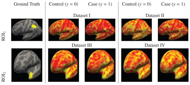
Synthetic Dataset: The two different regions of interests (ROIs) used for construction of the synthetic datasets are shown in yellow in the left most column. Examples of synthetically generated cortical thickness maps from the control and case groups are shown in the remaining columns. The regions and the simulated thickness maps are overlayed on the inflated surface of the left hemisphere of the common coordinate system. In gray we show the gyral patterns, where dark gray areas are sulci and light gray areas are gyri. We note that it is visually quite difficult to discern the difference between synthetic thickness maps of a healthy and a diseased sample.

We constructed four synthetic datasets each composed of 50 controls and 50 patients, so altogether of 100 samples. The control groups were constructed the same way for each dataset. The patient groups on the other hand had different ξ values and ROIs. The ξ value for datasets 1 and 3 was ξ = 0.085 and for dataset 2 and 4 it was ξ = 0.115. The first and second dataset are constructed based on ROI₁ shown in Figure 2. The third and fourth synthetic datasets are based on ROI₂ in the same figure. This corresponds to a signal-to-noise ratio (SNR) of 0.56 ± 0.05 for dataset 1, 0.75 ± 0.08 for dataset 2, 0.55 ± 0.08 for dataset 3 and 0.72 ± 0.12 for dataset 4. The SNR was calculated as the mean over the point-wise differences between the healthy and diseased divided by the standard deviation inside the ROI. Examples of synthesized thickness maps for each of the four datasets both from the control and the patient groups can also be seen in Figure 2. Similar to the ADNI, MCIC and COBRE datasets, the labels are set to be disease diagnosis represented with binary variables, i.e. 0 for the control group and 1 for the patients.

Additionally, we created two different sample sets for each synthetic dataset, a training and a testing dataset, each consisting of 100 samples. In each experiment, the first sample set was used to perform feature selection and optimize algorithmic parameters. For LASSO, Sparse SVC and Elastic Net, we then used the optimal parameters to train the algorithms on the first sample set and evaluated the prediction accuracy on the second sample set. For RFE-SVC, Random Forests and the proposed method, after feature selection we trained the algorithms on the first sample set using only the selected features and then again evaluated the prediction accuracy on the second sample set.

5.2. Algorithms for comparison

To provide an empirical comparisons with the state-of-the-art we used the following different methods in our analysis in addition to the proposed one:

1. Mass-univariate analysis with generalized linear models [1, 2] (Univariate)

2. LASSO [25]

3. Elastic Net [72]

4. Sparse logistic regression [16] (Sparse LR)

5. Sparse support vector classification [37] (Sparse SVC)

6. Random Forest with Gini Contrast [15] (RF Gini)

7. Stability Selection based on LASSO [41] (StabSel)

8. Recursive feature selection [40] with support vector regression or classification (RFE)

9. Shrinkage linear discriminant analysis [46] (SLDA)

10. Regression analysis by Mahalanobis-decorrelation [73] (CARS)

11. Shrinkage diagonal discriminant analysis [46] (SDDA)

Our pool of comparison methods includes representatives of a variety of important types of algorithms: linear, nonlinear, univariate, multivariate, sparse, ranking-based. In all the methods except the mass-univariate analysis, we either optimized the algorithmic parameters for highest prediction accuracy, as conventional, or if such an optimization was impossible we ran the algorithm with different parameter settings. This was the case for the following algorithms: RF Gini, StabSel, RFE, SLDA, SDDA and CARS. Both RF Gini and StabSel assign an importance measure to features for which determining a threshold is not trivial, but the measures can be used to rank the features. So, using these measures we ranked the features and used three different thresholds such that the top 15%, 50% and 85% of the features would be identified as relevant, respectively. The features that got 0 importance measure were not taken into account in this computation. RFE is an iterative algorithm that can also be used to rank features based on which iteration they get pruned out. Features that survive all iterations would have the top rank and those that get pruned out in the first iteration would get the last. As the other algorithms, it is not trivial to determine a threshold in this ranking. So, we used three different rankings where the features that had higher ranks than 1, 5 and 10 were identified as relevant, respectively. SLDA and SDDA compute correlation-adjusted t-scores, and CARS computes correlation-adjusted marginal correlation scores for each feature. In all of these algorithms the resulting scores are argued to be accurate variable importance measures. Therefore, they can be used to rank features. More importantly, authors in [46] and [73] provide details on how to threshold the variable importance measures by limiting the false discovery rate (FDR). In our experiments we used this strategy and used three different FDR thresholds, namely FDR < 0.8, FDR < 0.2 and FDR < 0.05. The first two limits are the values suggested by the authors in the respective articles.

For the experiments with univariate analysis, we first smoothed the individual cortical thickness maps using a smoothing kernel with 5 mm full-width-half-maximum on the common coordinate system. From the smoothed maps, we first computed the uncorrected maps using the Freesurfer software suite and thresholded these at p ≤ 0.05, 0.01 and 0.001. These results are presented with the acronym “Univariate”. We then performed two different corrections for multiple comparisons on the raw univariate maps. We applied family-wise error correction using Bonferroni’s method [3] and cluster-wise correction using the Monte Carlo simulations described in [8] with two different parameter settings: (voxel-wise threshold, cluster-wise threshold) = (0.01, 0.01) and (0.001, 0.001), which are common parameter settings used in various studies. These results are presented with the acronyms “Bonferroni” and “CWC” in the results section.

Lastly, we also experimented using another MVPA method within the knock-out algorithm instead of Random Forest. For this we used LASSO and refer to the resulting method as LASSO-KO in the results section. The tuning parameters for the LASSO component was set so as to maximize the prediction accuracy. The only tuning parameter that remained to be determined in LASSO-KO was C, which is used in the generalized intersection. We experimented using three different values, C = 3, 5, 7 mm. As the distance d(·, ·) in the generalized intersection we used the distance on the cortical surface, which can be computed using the triangulated mesh.

We used the “scikit-learn” python package [74] and “sda” and “care” R packages [46, 73] to implement all the competing state-of-the-art methods. The univariate analysis and the corresponding cluster-wise-correction was performed as implemented in the Freesurfer software suite (https://freesurfer.nmr.mgh.harvard.edu).

5.3. Parameter Settings for the Proposed Method

As discussed in Section 3.4 the proposed method has two parameters on its own and also inherits the parameters of the Random Forest algorithm. In all the experiments we used one set of parameters for the Random Forest algorithm. We set the number of trees to 500, number of minimum samples per leaf node to 10, subsampling ratio of the samples to 0.5 and the number of features used per node to 500. Additionally, for the forest variant we have used, the neighboring approximation forests, we needed to define the number of closest neighbors that will be used during predictions. This number indicates the number of samples that will be identified by the forest and used to predict the label of the test sample. We set this number to 15 for all the experiments based on the analysis given in [51]. We note that different parameter settings are also possible and we have set these parameters based on experience. Readers who are familiar with the Random Forest algorithm can use the parameter settings they prefer.

As for the tuning parameters of the proposed model, α and C, we have performed a sensitivity analysis with α = 0.01, 0.05 and C = 3 – 10 mm and provided its results in the supplementary material. Based on this analysis we present experimental results for all our data with α = 0.01 and C = 5 mm and 7 mm. We also applied the multiple comparisons correction step explained in Section 4 to correct the results obtained using the proposed method. As cluster-wise thresholds we experimented with 0.01 and 0.05.

5.4. Performance assessment

In the synthetic experiments we quantitatively assessed the performance of different algorithms. We compared the estimated relevant feature sets with the ground truth relevant features using sensitivity and DICE scores. We define the sensitivity s as

$$s=\frac{\text{TP}}{\text{TP}+\text{FN}}$$ (4)

and the Dice score d

$$d=\frac{\text{2TP}}{\text{TP}+\text{FN}+\text{FP}},$$ (5)

where TP stands for true positive (algorithm correctly identifies a feature as relevant), FP for false positive (algorithm identifies the feature as relevant while it is not), TN for true negative (algorithm correctly identifies a feature as non-relevant) and FN for false negative (algorithm identifies the feature as non-relevant while in reality it is relevant). We do not choose to present specificity values (given by $\frac{\text{TN}}{\text{TN}+\text{FP}}$) because due to TN ≫ FP they will always be very close to 1 and hence, it is not a discriminating measure for algorithm comparison in our case.

In case of the real data we can not measure the feature retrieval performance because the ground truth features are not available. Instead, we provide visual results and qualitatively compare the results from different methods as well as with the findings in the literature.

5.5. Reproducibility study

In addition to the performance evaluation on the synthetic and real datasets, we also tested the reproducibility of the proposed method and compared it to univariate tests. To this end, we chose one of the two lager data sets, the ADNI data set, and randomly subsampled it to create ten data sets each consisting of a group of 50 AD patients and an age and sex-matched group of 50 controls. We then performed univariate analysis as well as ran the proposed method on all the smaller subsets in the same fashion as was done on the entire data set.

We evaluated the reproducibility of the proposed method and the univariate tests based on two criteria. First, for each feature we computed the number of subsampled datasets where it gets identified as relevant. The ideal algorithm would be able to identify the same features in all the subsets. Second, we compared the relevant feature sets identified using the subsampled datasets with the sets identified using the entire dataset. This evaluation aims to display the effect of dataset size on the power of the algorithm.

6. Results and Discussion

In the following we present the results of our experiments and discuss them. We start with the experiments on the four synthetic datasets and then move on to the four real datasets. Finally, we present the outcome of our reproducibility study, describe the computational complexity of the proposed method and state its limitations.

6.1. Synthetic Datasets

We use the acronyms given in Section 5.2 to refer to different algorithms and the acronym “NAF-KO” to refer to the proposed method. We summarize the results in Figure 3, where we plot only the results of the best performing parameter settings for all the MVPA methods and the univariate techniques. Detailed results can be seen in the supplementary material provided with this article. For the proposed algorithm the figure displays the results obtained with α = 0.01, C = 5, 7 mm and a cluster-wise threshold of 0.05. Those parameters were chosen based on a sensitivity analysis provided in the supplementary material. Different graphs plot the results obtained in different datasets. In each graph the dashed vertical line separates uncorrected techniques from the ones corrected for multiple comparison.

Figure 3.

The sensitivity and Dice overlap on the four synthetic datasets for the best parameter combination of each algorithm. Methods that correct for the multiple comparison problem are on the right side of the dashed line. In each experiment, the training sample set set was used to perform feature selection and optimize algorithmic parameters. A full list of all results is provided in the supplementary material.

Observing the results in Figure 3, we note that the proposed method outperformed other MVPA methods in terms of DICE score across the board. This suggests that the proposed method indeed detects important features and not just adds more. In terms of sensitivity RFE, SLDA and SDDA yielded scores comparable to those of the proposed method. For RFE, the high sensitivity came at the expense of a substantial decrease in DICE score. The two algorithms specifically developed for high-dimensional correlated data, namely SLDA and SDDA, both achieved relatively high sensitivity as well as a relatively good Dice score in the synthetic datasets. Their performance was slightly lower than NAF-KO with and without cluster-wise correction in terms of feature retrieval.

The univariate analysis without correction achieved similar sensitivity scores as the proposed method on the second and third datasets and slightly lower values on the first and fourth dataset. The DICE scores of the uncorrected univariate analysis were substantially lower than the sensitivities indicating the weak specificity of uncorrected analysis.

We note that performances between datasets varied. The difference between the first (third) dataset and the second (fourth) dataset was due to the difference in the simulated effect sizes, ξ = 0.085 and ξ = 0.115. Smaller effect size naturally resulted in a more difficult problem. The difference between the first pair and the second pair of datasets was due to the location. ROI¹ had a larger variability in the normal anatomy. This characteristic was inherited by the simulated data making the first pair of datasets slightly more challenging than the second one.

The cluster-wise correction improved the DICE scores of both the univariate analysis and the proposed method. The Bonferroni correction on the other hand, being very strict, over-penalized the univariate analysis and resulted in very low sensitivity and DICE score. We observe that on the second dataset the univariate analysis with cluster-wise correction achieved the highest sensitivity and DICE scores (for the parameter setting (0.01, 0.01)). The proposed method’s results were also comparable to these results. For the first, third and fourth dataset on the other hand, the proposed method yielded higher DICE and sensitivity scores. This suggests that the multivariate analysis might be more advantegeous for smaller effect sizes and overall more difficult problems.

Furthermore, comparing LASSO-KO and NAF-KO we notice the advantages of using Random Forest within the proposed algorithm. The main drawback of LASSO-KO compared to NAF-KO arises from the sparsity of LASSO. Being sparse, LASSO aims to select very few but very discriminative features. When such strong features are present in the feature set, the algorithm can pick them up in any cross-validation fold and as such these features survive the intersection. However, when the feature set contains many but not very discriminative features, then LASSO might select different features in every fold and these features might not survive the intersection. This is the behavior we observe for LASSO-KO. The fact that the accuracy of LASSO-KO increased with increasing C also provides evidence for this behavior.

Lastly, we also present an analysis of the testing accuracy of the selected features on independently constructed test datasets in Figure 4 as well as in a table in the supplementary material. We observe that NAF-KO and other MVPA algorithms achieved very similar accuracies on all four datasets. The increase in feature selection accuracy did not translate into an increase in prediction accuracy. This result is not very surprising since we expect predictive models to select highly predictive features and discard any features that do not add to the prediction capability. As a result, the final model, although not accurate in feature retrieval, is still highly predictive. NAF-KO on the other hand, achieved both of these goals. It identified the relevant features with much higher accuracy while retaining good prediction capabilities.

Figure 4.

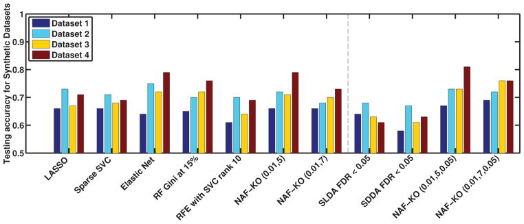
The accuracy of disease prediction of the four synthetic datasets for the best parameter combination of each algorithm described in Section 5.2 as well as corrected for multiple comparison to the right of the dashed line. In each experiment, the training sample set set was used to perform feature selection and optimize algorithmic parameters. Then the testing sample was used to evaluate prediction accuracy. A full list of all results is provided in the supplementary material as a table.

6.2. Real data

We present the results on the real datasets in Figures 5 and 6. Figure 5 displays the relevant feature sets detected by different MVPA methods on the OASIS dataset - i.e. features displaying age related variation. The features are plotted on the inflated surface of the left hemisphere of a common coordinate system (fsaverage5). We present the medial and the lateral views of the same surface in each image. On the surfaces, in gray levels we show the gyral patterns of the common coordinate system, where dark areas are sulci and light areas are gyri. The detected features, or more precisely the anatomical locations the relevant features are extracted from, are indicated with yellow. Under each image we denote the corresponding MVPA method and the parameter setting. In the last row we present the features detected with the proposed method. We applied the clusterwise correction on these results, however, it did not make any difference. For succinctness of discussion we show the results from other MVPA methods only on the OASIS dataset. Results obtained on the other datasets display similar behavior and they can be found in the supplementary material.

Figure 5. Relevant feature maps for different MVPA methods detected on the OASIS dataset.

Results are overlayed on the inflated surface of the left hemisphere of a common coordinate system (fsaverage5) in medial and lateral views. In gray we show the gyral pattern of the common coordinate system, where dark gray areas are sulci and light gray areas are gyri. The yellow regions are the relevant feature locations identified by each model. Underneath each image we detail which algorithm and which parameter settings were used.

Figure 6. Comparison of univariate analyses and NAF-KO.

In each dataset, the first rows show univariate results uncorrected and corrected for multiple comparisons using Bonferroni and a cluster-wise technique with two different parameter settings. The second rows display NAF-KO relevant feature results for two different (α,C) settings along with their accuracy maps (ADNI and OASIS) or corrected for multiple comparisons (MCIC and COBRE), where the cluster-wise correction threshold is set as 0.05. 23

In Figure 6, we show the univariate analyses results on all four real datasets together with the detection results of the proposed method. For all the datasets, in the first rows, we show the uncorrected univariate p-value maps (simply thresholded at 0.01) followed by the results of three different multiple comparisons correction methods: the Bonferroni and the two cluster-wise corrections, for which the voxel-wise and cluster-wise parameters are indicated inside parentheses in that order. The univariate results are color coded in the following way. Blue indicates negative correlation with the condition, while yellow and red indicate positive correlation. Light blue and yellow indicate a stronger effect, i.e. more significant p-values, than darker colors.

In the second rows we show the locations detected by the proposed method for two different parameter settings, which were selected based on their performance in the synthetic experiments. The parameter settings are indicated under each figure as (α,C). We present the results for the other parameter settings in the supplementary materials. The first two figures show the raw detection results without multiple comparisons correction for all the datasets. In the ADNI and OASIS datasets the multiple comparison correction did not change the results because the detected regions were large. Instead, in the third and fourth figures, we show accuracy maps, which at each vertex display the prediction accuracy Random Forest achieved in the iteration the feature for that vertex was knocked-out. In the figures yellow indicates the highest accuracy and dark red the lowest. The accuracy maps can be thought of as effect-size maps and they are comparable to the univariate maps but without distinction between positive and negative correlations.

In the MCIC and COBRE datasets the detected clusters were smaller and the multiple comparisons correction method of Section 4 pruned out some of the clusters. The third and fourth figures for the MCIC and COBRE datasets show the results after correction the results with a cluster-wise correction threshold of 0.05 (indicated under the corresponding images as the third value inside parentheses). The surviving clusters are shown in red. In the supplementary material we also provide the results for a cluster-wise threshold of 0.01. We do not show accuracy maps for the MCIC and COBRE datasets because for these the proposed method took at most 1 iteration of knock-out to stop.

In Figure 5 we observe that the difference between the proposed method and the other MVPA algorithms is striking. While NAF-KO identified almost all surface measurements of cortical thickness as relevant, the other algorithms produce much sparser relevant feature sets. LASSO, Elastic Net and RF-Gini all identified the most predictive features and discarded the rest. This behavior is as expected since all these methods aim to maximize prediction accuracy without any consideration for stability nor exhaustivity. Stability Selection, RFE and CARS yielded larger relevant feature sets for certain user-defined thresholds but also showed very large variation with respect to the thresholds. Numerous previous studies [38, 39, 75, 76] have analyzed the correlation between gray matter density and aging. Some have reported a global and linear relation [38, 39] while others have described non-linear effects [75, 76]. But regardless of the linearity of the effect, the literature seem to suggest that the aging effect covers the entire cerebral cortex. In light of these previous studies, NAF-KO’s results seem biologically more plausible than the maps produced by the other algorithms.

Contrary to the MVPA methods, the mass-univariate analysis on the OASIS dataset, shown in Figure 6(a), identified a much larger relevant feature set. Identified regions largely survived cluster-wise correction for multiple comparison as well. We note that the accuracy maps of NAF-KO and the correlation strength pattern that appeared in univariate analyses showed great similarities. This is not particularly surprising, since highly correlated regions also make good features for predictions.

Similar to aging, the effect of Alzheimer’s disease (AD) is also wide spread throughout the brain. AD’s effect on the cortical thickness has been documented in numerous studies [66, 67, 68]. Changes have been reported in several different regions among them the medialtemporal and tempoparietal regions as well as the posterior cingulate and precuneus in [66] and in another publication temporal, orbitofrontal and parietal regions [68]. In Figure 6(b) we observe that NAF-KO detected a very large relevant feature set in the ADNI dataset. Univariate analysis also detected large regions affected by AD. As in the OASIS dataset, the accuracy maps and the correlation strength maps computed using univariate analyses showed similar patterns. In fact, both of these maps showed similarities with the well-known Braak staging of AD described in [77]. In the NAF-KO accuracy maps, the values were the highest in areas related to Braak stage A, such as entorhinal cortex and other basal portions of neocortex, and decreased as it spreads all over neocortex as also described in Braak stages B and C.

One important point to note is that in both datasets, OASIS and ADNI, the proposed method detected larger regions than the univariate analyses. The difference was more prominent in the ADNI dataset. This behavior is actually similar to what we have seen in the synthetic datasets. The univariate analysis may have missed regions that have smaller effect sizes. Indeed, comparing the regions identified by CWC (0.001,0.001) with the accuracy maps obtained with NAF-KO, we see that the identified regions corresponded to the areas of high prediction accuracy. One common approach to improve the sensitivity of univariate analyses is to use larger smoothing kernels. We refer the reader to the supplementary material for further analyses on this point.

The results for the COBRE and MCIC datasets showed a different behavior. Previous studies on the relation of cortical thickness and schizophrenia have shown cortical atrophy in SCZ patients [78, 79, 80, 70, 81]. The effects were localized [70, 81], contrary to wide-spread effects seen in aging and AD. In particular, the work of Ehrlich et al. [70] also used the MCIC dataset in their analyses. The Figure 2 of their supplementary material shows the statistical maps of cortical thickness displaying regions of reduced thickness in schizophrenia patients compared to healthy controls and the regions are most pronounced in the frontal lobe, temporal cortex, inferior parietal lobe, and occipital cortex.

Observing the results shown in Figures 6(c) and (d), we can see that the relevant feature maps detected using the proposed method in the MCIC and COBRE datasets are much more localized compared to the results on ADNI and OASIS datasets. We observe some overlap between the regions identified by the univariate analyses and the proposed method. Only very few regions survived the multiple comparison correction for both methods. The proposed method detected larger regions as expected. Once again, this might have been due to the fact that univariate analysis can miss affected regions if the effect-size is small. Larger smoothing kernels may ameliorate this issue (see the supplementary materials for further analyses), at the cost of reducing the ability to localize effects, and removing effects with small spatial extents.

Another interesting point to note is that in both MCIC and COBRE datasets the detected regions were distributed across the hemisphere. These distributed patterns are examples that motivate global MVPA approaches as opposed to local approaches. By using the entire set of features all at once, global approaches are able to detect such patterns even though individual local regions by themselves may not display a strong correlation with the condition.

If we compare the results for MCIC (Figure 6(c)) to the areas of significant group differences in cortical thickness between healthy controls and SCZ subjects identified in [70] (Figure 2 in their supplementary material), we can see a large overlap of the regions identified by NAF-KO and Ehrlich et al. We note that Ehrlich et al. used a larger smoothing kernel in their analyses.

Finally, comparing the regions detected in the MCIC and COBRE datasets we see that NAF-KO with the parameter settings (0.01, 5 mm, 0.05) yielded some overlap. However, there were also regions that mismatched. This may have been due to the variation of the disease in schizophrenia as well as due to the small sample sizes in these datasets.

6.3. Reproducibility study

In the reproducibility study the identified relevant feature sets varied across the 10 different random subsets of the ADNI dataset for both the proposed method and the univariate tests. This variation is due to the difference in samples between the subsets and is not surprising. We quantified the variations for the different methods and provide the results in Figure 7.

Figure 7. Reproducibility of relevant features for random subsamples of ADNI.

(a): We display sum-maps where each vertex indicates the number of subsampled datasets the corresponding feature was identified as relevant in. A value of ten indicates the feature has been chosen in all random subsets, a value of one that it has been chosen in only one of the ten subsamples. The first row shows the results for univariate analysis with multiple comparisons correction with the cluster-wise technique for two different parameter settings. The second rows display the results for NAF-KO with multiple comparisons correction using the cluster-wise technique of Section 4. Two different parameter settings are shown for each method. NAF-KO demonstrated higher reproducibility across different random subsets. (b): We show the percentage of the original relevant feature set, which was identified using the entire dataset, that univariate analysis and NAF-KO were able to identify using the subsampled datasets. Stars indicate significant difference after paired two-sided t-tests, where ★: p < 0.05,★★: p < 0.01 and ★ ★ ★: p < 0.001.

In Figure 7(a), we display sum-maps, where at each vertex we indicate the number of subsets in which the feature at that vertex was identified as relevant. A value of ten indicates that the feature has been chosen in all the subsets and a value of one that it has been chosen in only one. In the first row, we show the results of univariate analysis with cluster-wise corrections, for which the voxel-wise and cluster-wise parameters are indicated inside parentheses in that order. In the second row we show the results of the proposed method with two different parameter settings, which were selected based on their performance on the synthetic experiments. The results for the proposed method were also corrected for multiple comparison using the cluster wise threshold of 0.05. The parameter settings are indicated under each figure as (α,C, cwt).

In Figure 7(b) we plot the relationship between the relevant feature sets identified using the subsampled datasets and the entire dataset. Specifically, we calculated the ratio of the number of relevant features identified in each subsampled dataset to the same number obtained using the entire dataset. The figure shows the box-plot where we plot the 10 ratios for each of the four different analyses (two different parameter settings for both the univariate and NAF-KO) as jittered points together with their mean and 95% confidence intervals for the mean. We performed paired two-sided t-tests between the univariate and NAF-KO results, where ★: p < 0.05,★★: p < 0.01 and ★ ★ ★: p < 0.001.

The results in Figures 7(a) and (b) show that overall NAF-KO demonstrated a higher reproducibility than univariate tests. In Figure 7(a) NAF-KO results display much larger regions with high sums (> 7) than the univariate results. Specifically, we note that the sizes of the regions that got identified in all of the subsampled datasets (regions with sum 10) are substantially larger for NAF-KO results than univariate analysis. This indicates that the proposed algorithm was more consistent across the different subsampled datasets. Moreover, the sum maps for NAF-KO were also consistent with the relevant features and accuracy maps identified using the entire ADNI dataset shown in Figure 6(b). Lastly, the box-plot in Figure 7(b) shows that the proposed method also retained a significantly higher percentage of the relevant features that were detected in the entire dataset in the ten random subsamples compared to the univariate tests. This suggest that the proposed algorithm may have more power for identifying relevant features in smaller data sets than univariate tests.

6.4. Computational complexity

The computational complexity of the proposed method is similar to other wrapper-type algorithms, such as recursive feature elimination. The computational bottleneck is the prediction-modelling component. In order to have a reliable accuracy estimate and set of selected features, we chose to perform 10 randomized 5 fold cross-validation experiments in each iteration. To speed up the computations one can use a computationally lighter estimation scheme, such as a single 5 fold cross-validation experiment, however, we would like to point out that this might come at the expense of decreasing accuracy.

In the current system we used C++ to implement the learning algorithm and Python to implement the knock-out iterations around the learning method. The exact execution time depends on the number of samples, number of features and how many iterations the algorithm will run for, which is not known a-priori. To provide some examples, on our synthetic dataset, which has 100 samples and 10242 features, each iteration takes 15 minutes and most experiments finished with only 2 iterations, while a few lasted for 3 iterations. So the longest experiment took 45 minutes to finish. On our largest dataset, which has 315 samples and 10242 features, each iteration took 25 minutes and the longest experiment took 11 iterations to finish, totalling up to 4 and a half hours. All the computations were performed on a single 64-bit Intel®Xeon®CPU running at 3.20 GHz with 7 Gb memory. The computations, in particular the 10 randomized 5 fold cross-validation experiments, can be fully parallelized and one may divide the computation times by almost 50.

6.5. Limitations

In general one of the limitations of MVPA algorithms compared to conventional univariate analysis is that MVPA methods are more complicated. This has been a barrier for many users unfamiliar with the underlying machine learning literature. But in recent years most algorithm developers make their software available for use and hence MVPA methods have become more accessible.

Comparing different MVPA algorithms with regard to usability we find that NAF-KO is not more complicated to use than Stability Selection [41] or recursive feature selection. And while it may seem that standard classification algorithms such as LASSO, Elastic Net or sparse support vector classification are easier to use, they also require cross-validation to set their internal parameters optimally. Regarding the limitations of using Random Forest as the underlying classifier compared to LASSO or support vector machines inside the knock-out framework, Random Forest seems to clearly outperform LASSO and has in general been extremely successful as a general purpose classification and regression method.

When compared to the computational complexity of univariate analysis or standard classification algorithms, the proposed method is obviously more demanding. However, we would like to point out that the increased reproducibility suggested by our experiments might justify the computationally more demanding nature of the method.

Finally, we would like to emphasize that by their nature, multivariate analyses cannot provide the same localized interpretation as univariate analysis. Multivariate methods jointly analyze a set of predictors and compute a statistical relationship between the condition and the entire set. The strength of the statistical relationship can only be attributed to the set as a whole rather than to the individual predictors alone. As a result, it is not possible to investigate the relationship of a single predictor with the condition. In contrast, univariate tests analyze each predictor in isolation and therefore, the strength of the relationship as well as its sign can be attributed to that particular predictor and further local interpretations become possible. However, our proposed multivariate method, as we have seen in the synthetic examples and the reproducibility study especially, can provide a more exhaustive feature set and can hence provide information that is not accessible by univariate analysis.

7. Conclusions and Future Work

We presented a new multivariate algorithm for relevant feature selection for neuroimaging studies. The proposed method is an iterative knock-out algorithm that uses Random Forests. The NAF-KO algorithm explicitly aims to construct an exhaustive set of relevant features with different mechanisms to attain exclusivity. In this respect, it differs from alternative MVPA methods proposed in the literature. Results on synthetic and real datasets presented in Section 6 demonstrate the advantages of the proposed method.

Furthermore, the real advantage of multivariate methods and specifically the proposed method over univariate analysis is shown in our reproducibility study. We see that NAF-KO achieves a much higher reproducibility than univariate analysis as presented in Figure 7. So whereas researchers often choose between either a univariate or a multivariate analysis or have difficulty consolidating the results achieved via univariate and multivariate methods, we feel that the proposed method can close the gap between the two approaches.

Future work includes the investigation of statistical guarantees about the recovery of relevant features. If parametric assumptions on the covariance can be made, then we would like to investigate if our proposed method can recover all relevant features with high probability.

Highlights.

• We propose an MVPA-based algorithm to identify all condition-related features.

• The algorithm retrieved relevant features at higher accuracy than other MVPA methods.

• It was in better agreement with univariate analysis results than other MVPA methods.

• Compared to univariate analysis, our method identified consistently larger regions.

• The proposed algorithm showed a higher reproducibility than univariate analysis.

References

- 1.Friston KJ, Holmes AP, Worsley KJ, Poline JP, Frith CD, Frackowiak RS. Statistical parametric maps in functional imaging: a general linear approach. Human brain mapping. 1994;2:189–210. [Google Scholar]
- 2.Ashburner J, Friston KJ. Voxel-based morphometry the methods. Neuroimage. 2000;11:805–821. doi: 10.1006/nimg.2000.0582. [DOI] [PubMed] [Google Scholar]
- 3.Bonferroni CE. Tipografia del Senato. 1935. Il calcolo delle assicurazioni su gruppi di teste. [Google Scholar]
- 4.Benjamini Y, Hochberg Y. Controlling the false discovery rate: a practical and powerful approach to multiple testing. Journal of the Royal Statistical Society. Series B (Methodological) 1995:289–300. [Google Scholar]
- 5.Storey JD, Tibshirani R. Statistical significance for genomewide studies. Proceedings of the National Academy of Sciences. 2003;100:9440–9445. doi: 10.1073/pnas.1530509100. [DOI] [PMC free article] [PubMed] [Google Scholar]
- 6.Worsley KJ, Marrett S, Neelin P, Vandal AC, Friston KJ, Evans AC, et al. A unified statistical approach for determining significant signals in images of cerebral activation. Human brain mapping. 1996;4:58–73. doi: 10.1002/(SICI)1097-0193(1996)4:1<58::AID-HBM4>3.0.CO;2-O. [DOI] [PubMed] [Google Scholar]
- 7.Andrade A, Kherif F, Mangin JF, Worsley KJ, Paradis AL, Simon O, Dehaene S, Le Bihan D, Poline JB. Detection of fmri activation using cortical surface mapping. Human brain mapping. 2001;12:79–93. doi: 10.1002/1097-0193(200102)12:2<79::AID-HBM1005>3.0.CO;2-I. [DOI] [PMC free article] [PubMed] [Google Scholar]
- 8.Hagler DJ, Jr, Saygin AP, Sereno MI. Smoothing and cluster thresholding for cortical surface-based group analysis of fmri data. Neuroimage. 2006;33:1093–1103. doi: 10.1016/j.neuroimage.2006.07.036. [DOI] [PMC free article] [PubMed] [Google Scholar]
- 9.Smith SM, Nichols TE. Threshold-free cluster enhancement: Addressing problems of smoothing, threshold dependence and localisation in cluster inference. NeuroImage. 2009;44:83–98. doi: 10.1016/j.neuroimage.2008.03.061. [DOI] [PubMed] [Google Scholar]
- 10.De Martino F, Valente G, Staeren N, Ashburner J, Goebel R, Formisano E. Combining multivariate voxel selection and support vector machines for mapping and classification of fmri spatial patterns. Neuroimage. 2008;43:44–58. doi: 10.1016/j.neuroimage.2008.06.037. [DOI] [PubMed] [Google Scholar]
- 11.Mourao-Miranda J, Bokde ALW, Born C, Hampel H, Stetter M. Classifying brain states and determining the discriminating activation patterns: Support vector machine on functional MRI data. NeuroImage. 2005;28:980–995. doi: 10.1016/j.neuroimage.2005.06.070. [DOI] [PubMed] [Google Scholar]
- 12.Kriegeskorte N, Goebel R, Bandettini P. Information-based functional brain mapping. Proceedings of the National Academy of Sciences of the United States of America. 2006;103:3863–3868. doi: 10.1073/pnas.0600244103. [DOI] [PMC free article] [PubMed] [Google Scholar]
- 13.Menze BH, Kelm BM, Masuch R, Himmelreich U, Bachert P, Petrich W, Hamprecht FA. A comparison of random forest and its Gini importance with standard chemometric methods for the feature selection and classification of spectral data. BMC bioinformatics. 2009;10:213. doi: 10.1186/1471-2105-10-213. [DOI] [PMC free article] [PubMed] [Google Scholar]
- 14.Sabuncu M, Van Leemput K. The relevance voxel machine (rvoxm): A self-tuning bayesian model for informative image-based prediction, Medical Imaging. IEEE Transactions on. 2012;31:2290–2306. doi: 10.1109/TMI.2012.2216543. [DOI] [PMC free article] [PubMed] [Google Scholar]
- 15.Langs G, Menze BH, Lashkari D, Golland P. Detecting stable distributed patterns of brain activation using gini contrast. NeuroImage. 2011;56:497–507. doi: 10.1016/j.neuroimage.2010.07.074. [DOI] [PMC free article] [PubMed] [Google Scholar]
- 16.Yamashita O, Sato M-a, Yoshioka T, Tong F, Kamitani Y. Sparse estimation automatically selects voxels relevant for the decoding of fmri activity patterns. NeuroImage. 2008;42:1414–1429. doi: 10.1016/j.neuroimage.2008.05.050. [DOI] [PMC free article] [PubMed] [Google Scholar]
- 17.Gaonkar B, Davatzikos C. MICCAI 2012. Springer; 2012. Deriving statistical significance maps for svm based image classification and group comparisons; pp. 723–730. [DOI] [PMC free article] [PubMed] [Google Scholar]
- 18.Rondina J, Hahn T, de Oliveira L, Marquand A, Dresler T, Leitner T, Fallgatter A, Shawe-Taylor J, Mourao-Miranda J. Scors - a method based on stability for feature selection and mapping in neuroimaging, Medical Imaging. IEEE Transactions on. 2014;33:85–98. doi: 10.1109/TMI.2013.2281398. [DOI] [PMC free article] [PubMed] [Google Scholar]
- 19.Mwangi B, Tian TS, Soares JC. A review of feature reduction techniques in neuroimaging. Neuroinformatics. 2014;12:229–244. doi: 10.1007/s12021-013-9204-3. [DOI] [PMC free article] [PubMed] [Google Scholar]
- 20.Rasmussen PM, Hansen LK, Madsen KH, Churchill NW, Strother SC. Model sparsity and brain pattern interpretation of classification models in neuroimaging. Pattern Recognition. 2012;45:2085–2100. [Google Scholar]
- 21.Konukoglu E, Ganz M, Van Leemput K, Sabuncu MR. Machine Learning in Medical Imaging. Springer; 2013. On feature relevance in image-based prediction models: An empirical study; pp. 171–178. [Google Scholar]
- 22.Amit Y, Geman D. Shape quantization and recognition with randomized trees. Neural computation. 1997;9:1545–1588. [Google Scholar]
- 23.Breiman L. Random forests. Machine learning. 2001;45:5–32. [Google Scholar]
- 24.Konukoglu E, Ganz M. ArXiv e-prints. 2014. Approximate False Positive Rate Control in Selection Frequency for Random Forest. [Google Scholar]
- 25.Tibshirani R. Regression shrinkage and selection via the lasso. Journal of the Royal Statistical Society. Series B (Methodological) 1996:267–288. [Google Scholar]
- 26.McIntosh A, Bookstein F, Haxby JV, Grady C. Spatial pattern analysis of functional brain images using partial least squares. Neuroimage. 1996;3:143–157. doi: 10.1006/nimg.1996.0016. [DOI] [PubMed] [Google Scholar]
- 27.McIntosh AR, Lobaugh NJ. Partial least squares analysis of neuroimaging data: applications and advances. Neuroimage. 2004;23:S250–S263. doi: 10.1016/j.neuroimage.2004.07.020. [DOI] [PubMed] [Google Scholar]
- 28.Krishnan A, Williams LJ, McIntosh AR, Abdi H. Partial least squares (PLS) methods for neuroimaging: a tutorial and review. Neuroimage. 2011;56:455–475. doi: 10.1016/j.neuroimage.2010.07.034. [DOI] [PubMed] [Google Scholar]
- 29.Friston KJ. Eigenimages and multivariate analyses. Human Brain Function. 1997 [Google Scholar]
- 30.Friston KJ, Frith CD, Frackowiak RSJ, Turner R. Characterizing dynamic brain responses with fMRI: A multivariate approach. NeuroImage. 1995;2:166–172. doi: 10.1006/nimg.1995.1019. [DOI] [PubMed] [Google Scholar]
- 31.Worsley KJ, Poline JB, Friston KJ, Evans AC. Characterizing the response of PET and fMRI data using multivariate linear models. NeuroImage. 1997;6:305–319. doi: 10.1006/nimg.1997.0294. [DOI] [PubMed] [Google Scholar]
- 32.Kriegeskorte N, Goebel R, Bandettini P. Information-based functional brain mapping. Proceedings of the National Academy of Sciences of the United States of America. 2006;103:3863–3868. doi: 10.1073/pnas.0600244103. [DOI] [PMC free article] [PubMed] [Google Scholar]
- 33.Zhang T, Davatzikos C. Odvba: optimally-discriminative voxel-based analysis, Medical Imaging. IEEE Transactions on. 2011;30:1441–1454. doi: 10.1109/TMI.2011.2114362. [DOI] [PMC free article] [PubMed] [Google Scholar]
- 34.Rondina J, Shawe-Taylor J, Mourao-Miranda J. Stability-based multivariate mapping using scors. Pattern Recognition in Neuroimaging (PRNI), 2013 International Workshop on; 2013. pp. 198–202. [DOI] [Google Scholar]
- 35.Haufe S, Meinecke F, Goergen K, Daehne S, Haynes JD, Blankertz B, Biessmann F. On the interpretation of weight vectors of linear models in multivariate neuroimaging. NeuroImage. 2014;87:96–110. doi: 10.1016/j.neuroimage.2013.10.067. [DOI] [PubMed] [Google Scholar]
- 36.Tipping M. Advances in Neural Information Processing Systems. Vol. 12. MIT Press; 2000. The relevance vector machine; pp. 652–658. [Google Scholar]
- 37.Bi J, Bennett K, Embrechts M, Breneman C, Song M. Dimensionality reduction via sparse support vector machines. The Journal of Machine Learning Research. 2003;3:1229–1243. [Google Scholar]
- 38.Pfefferbaum A, Mathalon DH, Sullivan EV, Rawles JM, Zipursky RB, Lim KO. A quantitative magnetic resonance imaging study of changes in brain morphology from infancy to late adulthood. Archives of neurology. 1994;51:874–887. doi: 10.1001/archneur.1994.00540210046012. [DOI] [PubMed] [Google Scholar]
- 39.Good CD, Johnsrude IS, Ashburner J, Henson RN, Fristen K, Frackowiak RS. A voxel-based morphometric study of ageing in 465 normal adult human brains. Biomedical Imaging, 2002. 5th IEEE EMBS International Summer School on; IEEE; 2002. p. 16. [Google Scholar]
- 40.Guyon I, Weston J, Barnhill S, Vapnik V. Gene selection for cancer classification using support vector machines. Machine learning. 2002;46:389–422. [Google Scholar]
- 41.Meinshausen N, Bühlmann P. Stability selection. Journal of the Royal Statistical Society: Series B (Statistical Methodology) 2010;72:417–473. [Google Scholar]
- 42.Yourganov G, Schmah T, Churchill NW, Berman MG, Grady CL, Strother SC. Pattern classification of fmri data: Applications for analysis of spatially distributed cortical networks. NeuroImage. 2014;96:117–132. doi: 10.1016/j.neuroimage.2014.03.074. [DOI] [PubMed] [Google Scholar]
- 43.Saeys Y, Inza I, Larrañaga P. A review of feature selection techniques in bioinformatics. bioinformatics. 2007;23:2507–2517. doi: 10.1093/bioinformatics/btm344. [DOI] [PubMed] [Google Scholar]
- 44.Awada W, Khoshgoftaar TM, Dittman D, Wald R, Napolitano A. A review of the stability of feature selection techniques for bioinformatics data. Information Reuse and Integration (IRI), 2012 IEEE 13th International Conference on; IEEE; 2012. pp. 356–363. [Google Scholar]
- 45.Clemmensen L, Hastie T, Witten D, Ersbøll B. Sparse discriminant analysis. Technometrics. 2011;53 [Google Scholar]
- 46.Ahdesmaki M, Strimmer K, et al. Feature selection in omics prediction problems using cat scores and false nondiscovery rate control. The Annals of Applied Statistics. 2010;4:503–519. [Google Scholar]
- 47.Haxby JV, Gobbini MI, Furey ML, Ishai A, Schouten JL, Pietrini P. Distributed and overlapping representations of faces and objects in ventral temporal cortex. Science. 2001;293:2425–2430. doi: 10.1126/science.1063736. [DOI] [PubMed] [Google Scholar]
- 48.Carlson T, Schrater P, He S. Patterns of activity in the categorical representations of objects. Journal of Cognitive Neuroscience. 2003;15:704–717. doi: 10.1162/089892903322307429. [DOI] [PubMed] [Google Scholar]
- 49.Pearson K, Lee A. Mathematical contributions to the theory of evolution. iii. regression, heredity and panmixia, Philosophical Transactions of the Royal Society of London. Series A. Containing Papers of a Mathematical or Physical Character. 1896;187:253–318. [Google Scholar]
- 50.Criminisi A, Shotton J, Konukoglu E. Decision Forests: A Unified Framework. Foundations and Trends in Computer Graphics and Vision. 2012;7 [Google Scholar]
- 51.Konukoglu E, Glocker B, Zikic D, Criminisi A. Neighbourhood approximation using randomized forests. Medical Image Analysis. 2013 doi: 10.1016/j.media.2013.04.013. [DOI] [PubMed] [Google Scholar]
- 52.Strobl C, Boulesteix A-L, Zeileis A, Hothorn T. Bias in random forest variable importance measures: illustrations, sources and a solution. BMC bioinformatics. 2007;8:25. doi: 10.1186/1471-2105-8-25. [DOI] [PMC free article] [PubMed] [Google Scholar]
- 53.Pereira F, Botvinick M. Information mapping with pattern classifiers: a comparative study. Neuroimage. 2011;56:476–496. doi: 10.1016/j.neuroimage.2010.05.026. [DOI] [PMC free article] [PubMed] [Google Scholar]
- 54.Breiman L, Adele C. [Accessed: 2014-07-28];Random forests - classification manual. 2008 http://www.stat.berkeley.edu/~breiman/RandomForests/cc_manual.htm.
- 55.John G, Kohavi R, Pfleger K. ICML. 1994. Irrelevant Features and the Subset Selection Problem. [Google Scholar]
- 56.Nichols TE, Holmes AP. Nonparametric permutation tests for functional neuroimaging: A primer with examples. Human Brain Mapping. 2002;15:1–25. doi: 10.1002/hbm.1058. [DOI] [PMC free article] [PubMed] [Google Scholar]
- 57.Fischl B. Freesurfer. Neuroimage. 2012;62:774–781. doi: 10.1016/j.neuroimage.2012.01.021. [DOI] [PMC free article] [PubMed] [Google Scholar]
- 58.Dale AM, Fischl B, Sereno MI. Cortical surface-based analysis: I. segmentation and surface reconstruction. Neuroimage. 1999;9:179–194. doi: 10.1006/nimg.1998.0395. [DOI] [PubMed] [Google Scholar]
- 59.Fischl B, Sereno MI, Dale AM. Cortical surface-based analysis ii: Inflation, flattening, and a surface-based coordinate system. Neuroimage. 1999;9:195–207. doi: 10.1006/nimg.1998.0396. [DOI] [PubMed] [Google Scholar]
- 60.Fischl B, Dale AM. Measuring the thickness of the human cerebral cortex from magnetic resonance images. Proceedings of the National Academy of Sciences. 2000;97:11050–11055. doi: 10.1073/pnas.200033797. [DOI] [PMC free article] [PubMed] [Google Scholar]
- 61.Fischl B, Sereno MI, Tootell RB, Dale AM, et al. High-resolution intersubject averaging and a coordinate system for the cortical surface. Human brain mapping. 1999;8:272–284. doi: 10.1002/(SICI)1097-0193(1999)8:4<272::AID-HBM10>3.0.CO;2-4. [DOI] [PMC free article] [PubMed] [Google Scholar]
- 62.Marcus D, Wang T, Parker J, Csernansky J, Morris J, Buckner R. Open access series of imaging studies (oasis): cross-sectional mri data in young, middle aged, nondemented, and demented older adults. Journal of Cognitive Neuroscience. 2007;19:1498–1507. doi: 10.1162/jocn.2007.19.9.1498. [DOI] [PubMed] [Google Scholar]
- 63.Salat DH, Buckner RL, Snyder AZ, Greve DN, Desikan RS, Busa E, Morris JC, Dale AM, Fischl B. Thinning of the cerebral cortex in aging. Cerebral cortex. 2004;14:721–730. doi: 10.1093/cercor/bhh032. [DOI] [PubMed] [Google Scholar]
- 64.Mueller SG, Weiner MW, Thal LJ, Petersen RC, Jack CR, Jagust W, Trojanowski JQ, Toga AW, Beckett L. Ways toward an early diagnosis in alzheimer’s disease: The alzheimer’s disease neuroimaging initiative (adni) Alzheimer’s & Dementia. 2005;1:55–66. doi: 10.1016/j.jalz.2005.06.003. [DOI] [PMC free article] [PubMed] [Google Scholar]
- 65.Jack CR, Bernstein MA, Fox NC, Thompson P, Alexander G, Harvey D, Borowski B, Britson PJ, Whitwell JL, Ward C, et al. The alzheimer’s disease neuroimaging initiative (adni): Mri methods. Journal of Magnetic Resonance Imaging. 2008;27:685–691. doi: 10.1002/jmri.21049. [DOI] [PMC free article] [PubMed] [Google Scholar]
- 66.Baron J, Chetelat G, Desgranges B, Perchey G, Landeau B, De La Sayette V, Eustache F. in vivo mapping of gray matter loss with voxel-based morphometry in mild alzheimer’s disease. Neuroimage. 2001;14:298–309. doi: 10.1006/nimg.2001.0848. [DOI] [PubMed] [Google Scholar]
- 67.Lerch JP, Pruessner JC, Zijdenbos A, Hampel H, Teipel SJ, Evans AC. Focal decline of cortical thickness in alzheimer’s disease identified by computational neuroanatomy. Cerebral cortex. 2005;15:995–1001. doi: 10.1093/cercor/bhh200. [DOI] [PubMed] [Google Scholar]
- 68.Lerch JP, Pruessner J, Zijdenbos AP, Collins DL, Teipel SJ, Hampel H, Evans AC. Automated cortical thickness measurements from mri can accurately separate alzheimer’s patients from normal elderly controls. Neurobiology of aging. 2008;29:23–30. doi: 10.1016/j.neurobiolaging.2006.09.013. [DOI] [PubMed] [Google Scholar]
- 69.Gollub RL, Shoemaker JM, King MD, White T, Ehrlich S, Sponheim SR, Clark VP, Turner JA, Mueller BA, Magnotta V, et al. The mcic collection: a shared repository of multi-modal, multi-site brain image data from a clinical investigation of schizophrenia. Neuroinformatics. 2013;11:367–388. doi: 10.1007/s12021-013-9184-3. [DOI] [PMC free article] [PubMed] [Google Scholar]
- 70.Ehrlich S, Geisler D, Yendiki A, Panneck P, Roessner V, Calhoun VD, Magnotta VA, Gollub RL, White T. Associations of white matter integrity and cortical thickness in patients with schizophrenia and healthy controls. Schizophrenia bulletin. 2014;40:665–674. doi: 10.1093/schbul/sbt056. [DOI] [PMC free article] [PubMed] [Google Scholar]
- 71.T. C. for Biomedical Research Excellence, The center for biomedical research excellence (cobre), 2014.
- 72.Zou H, Hastie T. Regularization and variable selection via the elastic net. Journal of the Royal Statistical Society: Series B (Statistical Methodology) 2005;67:301–320. [Google Scholar]
- 73.Zuber V, Strimmer K. High-dimensional regression and variable selection using car scores. Statistical Applications in Genetics and Molecular Biology. 2011;10:1–27. [Google Scholar]
- 74.Pedregosa F, Varoquaux G, Gramfort A, Michel V, Thirion B, Grisel O, Blondel M, Prettenhofer P, Weiss R, Dubourg V, Vanderplas J, Passos A, Cournapeau D, Brucher M, Perrot M, Duchesnay E. Scikit-learn: Machine learning in Python. Journal of Machine Learning Research. 2011;12:2825–2830. [Google Scholar]
- 75.Resnick SM, Pham DL, Kraut MA, Zonderman AB, Davatzikos C. Longitudinal magnetic resonance imaging studies of older adults: a shrinking brain. The Journal of Neuroscience. 2003;23:3295–3301. doi: 10.1523/JNEUROSCI.23-08-03295.2003. [DOI] [PMC free article] [PubMed] [Google Scholar]
- 76.Terribilli D, Schaufelberger MS, Duran FL, Zanetti MV, Curiati PK, Menezes PR, Scazufca M, Amaro E, Jr, Leite CC, Busatto GF. Age-related gray matter volume changes in the brain during non-elderly adulthood. Neurobiology of aging. 2011;32:354–368. doi: 10.1016/j.neurobiolaging.2009.02.008. [DOI] [PMC free article] [PubMed] [Google Scholar]
- 77.Braak H, Braak E. Neuropathological stageing of alzheimer-related changes. Acta neuropathologica. 1991;82:239–259. doi: 10.1007/BF00308809. [DOI] [PubMed] [Google Scholar]
- 78.Nesvåg R, Lawyer G, Varnäs K, Fjell AM, Walhovd KB, Frigessi A, Jönsson EG, Agartz I. Regional thinning of the cerebral cortex in schizophrenia: effects of diagnosis, age and antipsychotic medication. Schizophrenia research. 2008;98:16–28. doi: 10.1016/j.schres.2007.09.015. [DOI] [PubMed] [Google Scholar]
- 79.Goldman AL, Pezawas L, Mattay VS, Fischl B, Verchinski BA, Chen Q, Weinberger DR, Meyer-Lindenberg A. Widespread reductions of cortical thickness in schizophrenia and spectrum disorders and evidence of heritability. Archives of general psychiatry. 2009;66:467–477. doi: 10.1001/archgenpsychiatry.2009.24. [DOI] [PMC free article] [PubMed] [Google Scholar]
- 80.Schultz CC, Koch K, Wagner G, Roebel M, Schachtzabel C, Gaser C, Nenadic I, Reichenbach JR, Sauer H, Schlösser RG. Reduced cortical thickness in first episode schizophrenia. Schizophrenia research. 2010;116:204–209. doi: 10.1016/j.schres.2009.11.001. [DOI] [PubMed] [Google Scholar]
- 81.Tully LM, Lincoln SH, Liyanage-Don N, Hooker CI. Impaired cognitive control mediates the relationship between cortical thickness of the superior frontal gyrus and role functioning in schizophrenia. Schizophrenia research. 2014;152:358–364. doi: 10.1016/j.schres.2013.12.005. [DOI] [PubMed] [Google Scholar]
Associated Data
This section collects any data citations, data availability statements, or supplementary materials included in this article.