On Relationships Between Fixation Identification Algorithms and Fractal Box Counting Methods

Abstract

Fixation identification algorithms facilitate data comprehension and provide analytical convenience in eye-tracking analysis. However, current fixation algorithms for eye-tracking analysis are heavily dependent on parameter choices, leading to instabilities in results and incompleteness in reporting.

This work examines the nature of human scanning patterns during complex scene viewing. We show that standard implementations of the commonly used distance-dispersion algorithm for fixation identification are functionally equivalent to greedy spatiotemporal tiling. We show that modeling the number of fixations as a function of tiling size leads to a measure of fractal dimensionality through box counting. We apply this technique to examine scale-free gaze behaviors in toddlers and adults looking at images of faces and blocks, as well as large number of adults looking at movies or static images.

The distributional aspects of the number of fixations may suggest a fractal structure to gaze patterns in free scanning and imply that the incompleteness of standard algorithms may be due to the scale-free behaviors of the underlying scanning distributions. We discuss the nature of this hypothesis, its limitations, and offer directions for future work.

1 Introduction

Many natural phenomena exhibit fractal or self-similar properties. For example, in one of the earliest reports regarding the self-similarity of natural phenomena, Mandelbrot [1967] showed that the length obtained by measuring the coastline of Britain depends on the length of the ruler used to carry out this measurement. Since Mandelbrot [1967], hundreds of studies have been published demonstrating self-similar or fractal qualities in nature. Fractal properties have been found in the surfaces of sandstone and shale [Wong et al. 1986], the fracture surfaces of metals [Mandelbrot et al. 1984], the structure and distribution of rivers and river basins [Rodrguez-Iturbe and Rinaldo 1997], coasts and continents [Mandelbrot 1967; Mandelbrot 1975], and it seems everywhere in between, up to the perimeter of interstellar cirrus [Bazell and Desert 1988]. In ecology, fractal properties have been reported for the flight patterns of albatrosses [Viswanathan et al. 1996], foraging patterns of deer and bumblebees [Viswanathan et al. 1999], and even movement of amoebas [Schuster and Levandowsky 1996]. Not content to be confined to the natural world, fractal analysis has been applied to economics [Mandelbrot 1999], the artwork of Jackson Pollock [Taylor et al. 1999], and investigations into the topology of the internet [Faloutsos et al. 1999].

A few research groups have examined power laws in eye movements. Notably, Brockmann and Geisel have developed a theoretical framework for describing the distributional properties of eye-movements as Lévy flights. Preliminary results seem to support their model [Brockmann and Geisel 1999; Brockmann and Geisel 2000]. Similarly, Boccignone and Ferraro [2004] describe a theoretical model which grounds gaze patterns in terms of low-level features and scene complexity, using a weighted Cauchy-Lévy distribution for jump lengths. Shelhamer, in a series of studies, has demonstrated that predictive saccades exhibit long-term correlations and fractal properties [Shelhamer 2005c; Shelhamer 2005a; Shelhamer 2005b; Shelhamer and Joiner 2003]. Aks et al. [2002] report similar findings in a search task when looking at the distance between fixations, a value which is related to saccade amplitude. Liang et al. [2005] use detrended fluctuation analysis to examine the scaling exponents of saccade velocity in microsaccades. In this paper, we will take advantage of the fractal properties of eye movement, and develop a fixation identification method using box counting.

Understandably, there has been a great deal of interest in the potentially fractal nature of human scanning patterns. Qualitatively, power law dynamics in two dimensional trajectories yield movements that bear a striking resemblance to eye movements. For example, in Figure 1 we employ an idealized model to demonstrate saccade generation. We generated saccades amplitudes in power law distribution, with the duration of each saccade being proportional to the square root of its amplitude, following the square-root main saccade rule proposed by Lebedev et al. [1996]. The resulting trajectories seem to qualitatively share more similar qualities with real eye movement patterns than trajectories generated with other distributions, e.g. normally distributed step-lengths (Figure 1).

Figure 1.

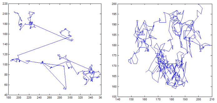
Left: Stimulated scan path with power-law step sizes. Right: Simulated scan path with normally distributed steps.

It is important to note that all of these studies exclusively focus on the power-law behavior of saccades. From a data analytic viewpoint there is a strong relationship between saccades and fixations [Salvucci and Goldberg 2000], where saccade detection is often regarded as an inverse process to fixation identification (i.e. what is not a fixation is a saccade or lost data). Because of this relationship, scale free behaviors in saccades ought to be associated with scale free behaviors in fixations. Interestingly, in previous publications that examined the parameters for fixation identification, Shic et al. [2008a; 2008b] showed that no natural discontinuities or multimodality existed in the relationship between fixation identification thresholds and fixation statistics. These results suggest that there is a smooth property to these fixation statistics, which may be related to scale free dynamics in viewing patterns.

In this paper, we use these insights to conduct a novel analysis on the relationship between scale free behaviors in natural eye scanning patterns and fixation identification algorithms. Specifically, we show that aggregation of results from multiple applications of a fixation identification algorithm bears striking similarity to box counting techniques that are used in fractal dimensionality calculations. We examine the nature of this result and test the model on scanning patterns of children and adults. We then discuss the relationship between this model and our previous work that examines ties between fixation identification algorithm parameters and fixation statistics. Finally, we conclude with a discussion of the nature of our hypothesis, the limitations of our work and of the hypothesis, and offer suggestions for future research directions.

2 Fractal dimensionality as computed through box counting

Mandelbrot applied the box counting method to Britain coastline measurement and showed that a self-similar power law connects the coastline length L and the scale unit s employed in its measurement:

$$L(s)~s^{-\alpha }$$ (1)

where the exponent α is positive if L increases as s decreases. To illustrate the box counting technique [Schroeder 1999], We extract the coastline of Great Britain from a postal map (UK postal areas, 2008) and replicated the well known results first highlighted by Mandelbrot [1967], in Figure 2.

Figure 2.

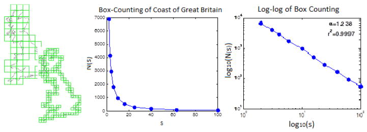
Left: Simple Box-counting of the coast of the U.K. The number of boxes needed to cover the coastline increases as a power law of the inverse of the size of the covering boxes. Middle: Number of boxes, N(s), of side-length s necessary to cover the coast of Great Britain. Right: log-log plot of left graph, showing a very linear relationship, suggesting a power law for the relationship between N(s) and s.

Dimensionality is an important property of fractals, such as the Hausdorff dimension. Given N(s) is the minimum number of disks of diameter s needed to cover a contour fractal, the Hausdorff dimension can be calculated:

$$D=\underset{s\to 0}{lim}\frac{\mathit{logN}(s)}{\mathit{log}(1/s)}$$ (2)

If we measure L in this manner, N(s) equals L(s)/s and the exponent −α in Equation 1 is equal 1 − D. Thus, the Hausdorff dimension is given by D = 1 − (−α), which, for α > 0, will exceed 1. For a smooth curve, D = 1; and for a smooth surface the number N of covering disks is proportional to 1/s² and therefore D = 2. D lies between 1 and 2 gives a infinitely long curve that is more than a one-dimensional object, but without being a two dimensional area, since the curve does not fully cover an area [Schroeder 1999].

In box counting, we superimpose a fixed grid of boxes of particular lengths, which is equivalent to the disk in Hausdorff’s method, to count the number of boxes N(s) which contain any of the coastline. As we can see from Equation 2, when s becomes very small, logN(s)/log(1/s) converges to a finite value, the Hausdorff dimension D. Mandelbrot [1967; 1983] publicized the Hausdorff dimension of difference coasts and 2–dimentional borders, showing that the dimensions ranged from smooth D ~ 1 for the west coast of South Africa, a ragged D ~ 1.3 for the west coast of Britain, with the distinction of the highest Hausdorff dimension going to Norway with a D ~ 1.52.

3 Multi-scale application of Fixation Identification Alorithms and Fractal Box Counting

Though box-counting is typically associated with boxes, the covering object need not be a box [Falconer 2003; Klinkenberg 1994]. In this section, we discuss how this insight furthers our understanding of the relationships between fixation identification algorithms and box counting methods.

A standard distance dispersion algorithm operates with two thresholds [Salvucci and Goldberg 2000; Shic et al. 2008b]. The first, a spatial parameter d_max, is the largest distance which any points within a set of consecutive points obtained from an eye tracker are separated. Moving outside of this range by any additional point added temporally to the end of the consecutive set of points ends the fixation, and starts a potential new fixation. The second thresh-old, t_min, represents the shortest time that a fixation may last. Any fixation that is determined to have a temporal extent less than t_min is considered to be non-physiological and is thus discarded. For simplification of our discussion, in this paper we will assume t_min = 0ms, though we will return to this point in our discussions of limitations.

It is important to note that most standard fixation identification algorithms are greedy by nature. That is, as many points are added to a growing potential fixation as possible, until the spatial threshold is exceeded. At the top panel of Figure 3, we see how the greedy distance fixation identification algorithm dissects a scanpath. The algorithm begins by identifying a candidate point and then grows as far as it can, temporally, until the next point is d_max away from some point already covered by the spatio-temporal cylinder. It then begins at the next valid point and repeats. The total number of cylinders needed to cover the trajectory is the total number of fixations. Thus the distance algorithm, viewed from this light, is a temporally-greedy version of box counting.

Figure 3.

Effect of modifying spatial parameters on standard greedy dispersion fixation algorithms. The gaze trajectory is shown moving through time vertically and projects onto the face image above and below. Top Left: With a large spatial parameter the cylinder covering the gaze trajectory is thicker, and fewer cylinders are needed to cover the trajectory. Top Right: With a smaller spatial parameter more cylinders are necessary. Representative example of a single trial. Bottom Left: Number of fixations N(s) as a function of s, the size of the spatial parameter for the distance algorithm (i.e. the maximal separating distance between points). Bottom Right: log-log plot of the bottom left plot. The line between points shows the theoretical line calculated by least-squares fit of a line to the log-transform of the set of points.

A distance dispersion algorithm using cylinders was applied to cover an eye movement trajectory in Figure 3. The sampling rate of eye tracking system is consistent, therefore the temporal dimension of the eye movement trajectory was not discarded, but instead, was compressed in a way that only the adjacent temporal sequence was kept. With a compressed temporal dimension, the fixation number counting is very similar to box counting of coastline length. We examined the number of fixations N(s) as a function of the spatial constraint parameter s = d_max under the distance-dispersion fixation identification algorithm.

$$N(s)=A{s}^{-\alpha }$$ (3)

The bottom area of the cylinder is determined by its diameter, and we have no maximum or minimum duration of this fixation identification algorithm, so the height of the cylinder can be arbitrary, and the diameter of the bottom surface of the cylinder s is the factor determining the counting results.

4 The Scaling Exponent of Free-scanning in Children and Adults

We presented pictures of faces or block designs to 15 typically-developing children (TD) at age 26.5 ± 4.2 months. Each image, including the grey background, was 12.8° x 17.6°. Eye-tracking data were obtained simultaneously with a SensoMotoric Instruments IView X RED table-mounted 60Hz eye-tracker. Stimulus images were preceded by a central fixation to refocus the child’s attention and were then displayed as long as was required for the child to attend to the image for a total of 10 full seconds. Actual trials could last longer than 10 seconds; however, to maintain comparability, only the first 10 seconds of stimulus presentation were analyzed in this study. Subsequently, 46 trials were admitted for blocks and 29 trials for faces (75 trials total). A representative example of one trial is shown in the bottom panels in Figure 3. Theoretically recording a trajectory continuously is necessary for us to measure the true scaling exponent of the eye movement data. As a coarse approximation to continuous measurement and to provide comparability across the experiments in this section, we apply linear interpolation to achieve approximately 1000Hz data (1ms sampling interval) for all data analysis here.

The average R² of the log-log linear regression was .98 (with standard error σ = 0.01), with the minimum fit on any of the 75 trials being R² = 0.94. The scaling exponent α differed (F = 4.3, p < 0.05) between blocks (α = 1.28(±0.17)) and faces (α = 1.19(±0.17)). The constant term (A in Equation 3) is approximately the log of the total amount of time spent in scanning and also differed (F = 7.4, p < 0.01) between blocks (A = 4.33(±.28)) and faces (A = 4.14(±0.33)). A representative comparison is shown in the top panel of Figure 4. We note that there appears to be individual variability in the scaling exponents, suggesting potentially different scanning strategies for different individuals or differential interactions between participants and presented stimuli.

Figure 4.

Representative example of a single trial. Log-log plot showing scaling between fixation size and fixation numbers. Top: Children data. Bottom: Adult data. Left: Faces trials. Right: Blocks trials. Note the stair-casing on the top left plot is due to discretization (i.e. low counts at high spatial scales.

To examine the nature of scanning on these stimuli in adults, we present the same set of stimuli on an Eyelink remote eye tracking system (SR Research) with 500Hz sample rate. Images span a visual angle of 13.4° x 17.8° vertically and horizontally in the center of a 22 inches screen, and each trial lasts 10 seconds. We have preliminary results of an adult participant, as shown in the lower panel of Figure 4. The average R² of the regression was 0.99 (σ = 0.015), with the minimum 0.96 on any of the 8 trials. The scaling exponent was α = 1.24 with σ = 0.06 for face trials, and the exponent was α = 1.13 with σ = 0.05 for block trials.

Data set 3 reflected 14 adults free viewing 10 trials of human face images with grey background using a SR Eyelink system, the same stimuli and eye tracker as in our data set 2. This scaling exponent α = 1.21(±0.19) is also consistent with the face section in data set 1.

We applied this analysis to an online database [Dorr et al. 2010] (data set 4), which includes eye movement data from 54 subjects for 18 outdoor scenes, 2 Hollywood trailers, and static images taken from the outdoor scenes, with sampling rate of 250Hz. The average exponent were α = 1.22 ± 0.14 for the Hollywood movies, 1.09 ± 0.09 natural movies, 1.15 ± 0.12 for repetitive, 1.04 ± 0.11 for static images, 1.14 ± 0.08 for stop motion movies and 1.06±0.11 additional stimuli respectively in the database. The average and distribution of the individual trials is plotted in box plots in Figure 5. We used a one way ANOVA with Bonferroni correction and find there is significant difference between these conditions (with p < 0.015), except between repetitive and stop motion movies(p = 1). It is worth noticing that the average R² of the log-log linear regression was R² = 0.99 (with standard error σ = 0.01). The high R² of regression shows the large data set still follows the power-law property.

Figure 5.

The calculated scaling exponent of eye movement of six different stimuli type in a database. Significant differences are found between these groups, except for repetitive and stop motion stimuli pair.

5 Number of fixations N(s) and mean fixation duration t_dur

If we assume the total amount of time spent in fixations stays constant, since the mean fixation duration is the total amount spent in fixations divided by the number of fixations, we can approximate the mean fixation duration t_dur as:

$$t_{\mathit{dur}}(t_{min},s)=\frac{T_{\mathit{total}}}{A{s}^{-\alpha }}$$ (4)

where T_total is the total time spent in fixations. Given that we have conducted this analysis with no minimum fixation duration for the distance-dispersion algorithm, i.e. t_min = 0 ms, no data should be lost to saccades when calculating the total fixation duration. If T_total is constant, then the inverse of the number of fixations N(s) should appear linear without log-transformation. This is in fact the case, as on the left of (Figure 6). It appears that linear trend seen for mean fixation dependence on spatial thresholds s, as in previous cylinder counting work.

Figure 6.

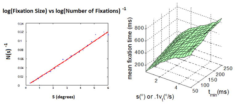
Left: Inverse of the number of fixations as a function of the scale of analysis. Right: Mean fixation duration of children viewing faces for different algorithms as a function of spatial and temporal parameters.

To further examine how these parameters correspond to distribution aspects of scanning, we conducted a simple linear interpolation model (SLIM) as proposed in [Shic et al. 2008a], with three coefficients being used to fit the mean fixation duration t_dur : a temporal slope, slope_t, a spatial slope, slope_s, and an offset, t0:

$$t_{\mathit{dur}}(t_{\mathit{min}},s)={\mathit{slope}}_t·t_{\mathit{min}}+{\mathit{slope}}_s·s+t0$$ (5)

The mean fixation duration of children viewing faces was calculated and plotted on the right side of Figure 6, and the coefficients of the SLIM are listed in Table 2. It is approximately linear in terms of both slope_s and slope_t.

Table 2.

Linear regression coefficients (slope_t, slope_s, and t₀) and regression explained variance (R2) of mean fixation duration for distance dispersion, and two different stimulus types (Faces and Blocks).

Distance-Dispersion Algorithm
slopet		slopes		t0		R2
Face	Block	Face	Block	Face	Block	Face	Block
0.67	0.74	142	175	83	−2	.981	.997

Since in this specific case, we have t_min = 0, we can eliminate the partial derivative of t_min, and the spatial coefficient slope_s can be calculated as the derivative of the Equation 4:

$${\mathit{slope}}_s=\frac{{dt}_{\mathit{dur}}}{ds}=K{s}^{\alpha -1}$$ (6)

We can see that if α = 1, the slope_s will be equal to the constant K. In our previous fractal dimensionality analysis, we found that both in adults and children’s free view eye movement, the exponent term α, which is equivalent to the fractal dimensionality, is close to 1.

Given the total time is constant, the inverted number of fixations is equivalent to mean fixation duration. The linearity between the log of box size and the log of fixation time is consistent with the flat plane slope in the dimension of s. The fractal dimension analysis also supports the linear model we used, as described in Equation 5.

The temporal coefficient in Equation 5, slope_t, characterizes how the mean fixation duration increases as the minimum time requirement t_min increases. A larger temporal slope counter-intuitively implies a greater loss of data: by removing fixations with shorter durations, the average fixation duration tends to increase. This process explains the discrepancy in temporal slopes for the velocity algorithm as compared to dispersion algorithms (Table 2). The temporal constraint for velocity algorithms is a pure rejection criterion; by comparison, dispersion algorithms have a chance to partially recover a fixation as the candidate fixation window slides. In terms of scanpath effects, a larger temporal coefficient implies more non-recoverable short-time fixations, i.e. short time fixations which are separated by large distances. A full analysis of this coefficient will require an analogous study examining the distribution of the durations of fixations. Should this distribution be found to have a particularly simple form, as we might expect, then the lost time to saccades should be proportional to the integral of the duration distribution up until t_min.

We should note that the implications of grounding mean fixation duration with a power-law for the number of fixations would suggest that mean fixation duration is not exactly linear, though for practical purposes it may be well modeled by a plane. The duration offset, t0, in this case, the offsets observed may be associated with errors caused by matching nonlinearities in the mean fixation duration. If we examine the behavior of children in Table 2, there is a modulation of coefficients as the stimulus changes from faces to blocks, and a swap of these relationships between our adult data (data set 2). Again, an examination of these effects are topics for further investigations, but we note that specific interpretations of the scaling exponent also will be related to interpretations of average fixation durations in general [Wass et al. 2013], given the relationships described in Equation 6.

6 Amplitude spectrum of natural images

If fractal patterns are associated with saccade and fixation behaviors, a natural question is to ask: what is the source of these patterns, and how did these behaviors evolve to come to be? Some work suggests that the answer to this question stems from the nature of the natural visual world itself. For instance, the amplitude spectrum of natural images has also been found to obey, on average, a 1/f power-law relationship, with f the spatial frequency [Field 1987; Burton and Moorhead 1987; Tolhurst et al. 1992] though there is considerable variation across image classes [Torralba and Oliva 2003]. Similarly, the images that we presented to the participants in our experiments also maintain these relationships, though the power law relationship between spatial frequency and amplitude is different for different stimuli classes (Figure 7). These findings offer a tantalizing hypothesis that the scaling behaviors of properties of visual images may be tied to the scaling behaviors of eye movements.

Figure 7.

Amplitude spectrum of the images used in our study. Top: amplitude spectrum for faces, with α = 1.59, R² = .998; Bottom: amplitude spectrum for blocks, α = 1.40, R² = .987.

7 Discussion

To overcome some of the limitations of our specific equipment and experimental setup, we used eye tracking data from four data sets, one online database and three studies carried out in our lab. These data sets include three different eye tracking systems, stimuli including both movies and static images, and participants from two age groups (toddlers and adults). Across these samples the same kind of linearity was observed between the log of fixation size and the number of fixations, suggesting a power law dependence between them. The exponent of adults’ data is of a similar magnitude as the exponent in the children’s study, though we note that the variability of the exponent seems to be pervasive across even individual trials, suggesting that it is not a stable property of individuals, but rather a property of interactions between the individual and the stimuli. Further work will have to decode the exact relationships between observed scaling exponents, individual characteristics, and stimulus properties.

Regarding the last point, it is an open question whether the power law statistics of images under view correlate with the scaling parameters of natural scanning. Given the lawful behavior of scaling in the scanning patterns of our participants, and the work accomplished by previous researchers, examining these properties within the context of our analytical framework may yield new perspectives on patterns of attention across development and the general relationship between attention and cognition.

Eye movement patterns are task relevant, whereas cognitive experiments usually have very different eye movement patterns as compared with psychophysical experiments. The fixation properties we calculated could also be relevant to our free-viewing task. It might be possible that the free-viewing aspects of the experiment are responsible for the simple structure we observe for mean fixation duration, and that the imposition of any greater experimental structure would break this effect. However, it is important to note that revealing this would not be possible except by charting parameters as we have suggested.

Additional limitations of this work include the fact that we are using binning and log binning to capture exponents related to scaling behaviors. This is a known limitation that has plagued much of the work examining the fractal properties of natural behaviors [Edwards et al. 2007]. It is likely that maximum likelihood estimation would improve the stability of our statistics, and this is a likely direction for future work. However, the main point of this paper is not that scanning patterns necessarily follow a Lévy flight or power-free behavior in general, but rather that within a specific range of parameters, scanning patterns and scale free behavior seem to well model the curves, and this modeling brings light to previous work that has noted linear relationships between parameters and fixation identification statistics. In addition, our results lends additional support to the idea that fixation properties are highly dependent on parameter choices in general, and obey a continuous dependence on these parameter choices. Though fixation statistics such as the mean fixation duration and the number of fixations play a prominent role in the interpretation of psychological and cognitive constructs, our work suggests that caution may be warranted, as any specific selection of parameter choices will vary the reported properties in a systematic fashion.

As a final example of this point, we consider the actual effects of t_min on the power law behaviors observed. If we manipulate t_min to be anything other than 0, we begin to see nonlinearities form in the number of fixations. An example of this phenomenon is shown in Figure 8, where we can see with t_min = 20ms the log of the fixation spatial parameter and versus the log of the number of fixations looks like an inverted V. The nonlinearity observed here is likely due to the specific properties of fixation identification algorithms. As the spatial parameter decreases, fixations will have smaller and smaller spatial widths, confining the number of fixation points that are likely to comprise individual fixations. Because the number of points within each fixation is reduced, the average time spent within each fixation will also decrease, all things being equal.

Figure 8.

With t_min = 20ms, nonlinearity can be observed in high density sampled data (500Hz) in adult’s free viewing

At some lower limit, microsaccadic behavior, tremor, and oculomotor drift begin to impact fixation statistics, as does the general presence of experimental noise, as described in Martinez-Conde et al.’s papers [2009 [2013]. In any event, the interaction between these temporally shorter fixations and any temporal minimum threshold on fixations will tend to throw out these small fixations, leading to the curvature observed. It is not clear as of yet how this phenomenon should be modelled, and it is not clear how the mean fix-ation duration is impacted within this range. While it is inversely related to the number of fixations, it is also affected by the total recording time, which is steadily decreased in the presence of more fixation rejections. What is clear is that if t_min truly makes physiological sense, there appears to be a limit by which, depending on the spatial parameter, power law dynamics may no longer hold. This is an area of ongoing investigation which should lead to better, more stable measures for use with eye tracking and thus more robust and replicable interpretations of associated cognitive and behavioral phenomenon.

8 Conclusion

We have adopted standard fixation algorithms to perform box-counting, a technique for measuring fractal dimension. We have shown that the scanning patterns of typically developing toddlers may have fractal qualities. We suggest that scale-free qualities of the scan pattern distribution may be one reason why an optimal set of parameters for fixation identification does not exist. We note that although other distributions may fit the scanning pattern data better [Edwards et al. 2007], a simple power law also represents the data well. Regardless of the exact underlying statistical distribution, it is clear that scanning patterns exhibit lawful, smooth and continuous properties. It is our hope that future studies with larger populations and extended experimental conditions will bear out the main results of this study and provide further insights into the nature of our findings.

Table 1.

Four data set we applied. The second column is the stimuli; the third column is the participant number and their age group; the fourth column is the sampling interval after linear interpolation; the fifth column alpha is the scaling component (fractal dimensionality); the sixth column is the A value; the R2 is the R square of the log-log linear regression.

Data set	Stimuli	Participants	alpha	A	R2
1	Faces	13 Toddlers	1.19	4.14	0.98
	Blocks	13 Toddlers	1.28	4.33	0.98
2	Faces	1 Adult	1.24	3.78	0.99
	Blocks	1 Adult	1.13	3.52	0.99
3	Faces	14 Adults	1.21	3.38	0.98
4	Hollywood Movies	54 Adults	1.22	4.46	0.99
	Natural Movies	54 Adults	1.09	4.09	0.99
	Repetitive	54 Adults	1.15	4.16	0.99
	Static Images	54 Adults	1.04	3.02	0.98
	Stop Motion Motives	54 Adults	1.14	4.09	0.99
	Additional	54 Adults	1.06	3.17	0.98

References

- Aks DJ, Zelinsky GJ, Sprott JC. Memory across eye-movements: 1/f dynamic in visual search. Nonlinear Dynamics, Psychology, and Life Sciences. 2002;6(1):1–25. [Google Scholar]
- Bazell D, Desert FX. Fractal structure of interstellar cirrus. Astrophysical Journal. 1988;333:353–358. [Google Scholar]
- Boccignone G, Ferraro M. Modelling gaze shift as a constrained random walk. Physica A: Statistical Mechanics and its Applications. 2004;331(1–2):207–218. [Google Scholar]
- Brockmann D, Geisel T. Are human scanpaths levy flights? artificial neural networks. ICANN 99. Ninth International Conference.1999. [Google Scholar]
- Brockmann D, Geisel T. The ecology of gaze shifts. Neurocomputing. 2000;32(33):643–650. [Google Scholar]
- Burton GJ, Moorhead IR. Color and spatial structure in natural scenes. Applied Optics. 1987;26(1):157–170. doi: 10.1364/AO.26.000157. [DOI] [PubMed] [Google Scholar]
- Dorr M, Martinetz T, Gegenfurtner K, Barth E. Variability of eye movements when viewing dynamic natural scenes. Journal of Vision. 2010;10(10):1–17. doi: 10.1167/10.10.28. [DOI] [PubMed] [Google Scholar]
- Edwards AM, Phillips RA, Watkins NW, Freeman MP, Murphy EJ, Afanasyev V, Buldyrev SV, da Luz MGE, Raposo EP, Stanley HE, Viswanathan GM. Revisiting lvy flight search patterns of wandering albatrosses, bumblebees and deer. Nature. 2007;449:1044–1048. doi: 10.1038/nature06199. [DOI] [PubMed] [Google Scholar]
- Falconer K, editor. Fractal Geometry - Mathematical Foundations and Applications. 2. England: John Wiley & Sons, Ltd, Western Sussex; 2003. [Google Scholar]
- Faloutsos M, Faloutsos P, Faloutsos C. On power-law relationships of the internet topology. Proceedings of the conference on Applications, technologies, architectures, and protocols for computer communication; 1999. pp. 251–262. [Google Scholar]
- Field DJ. Relations between the statistics of natural images and the response properties of cortical cells. J Opt Soc Am A. 1987;4(12):2379–2394. doi: 10.1364/josaa.4.002379. [DOI] [PubMed] [Google Scholar]
- Klinkenberg B. A review of methods used to determine the fractal dimension of linear features. Mathematical Geology. 1994;26(1):23–46. [Google Scholar]
- Lebedev S, Gelder PV, Tsui WH. Square-root relations between main saccadic parameters. Invest Ophthalmol Vis Sci. 1996;37(13):2750–2758. [PubMed] [Google Scholar]
- Liang JR, Moshel S, Zivotofsky AZ, Caspi A, Engbert R, Kliegl R, Havlin S. Scaling of horizontal and vertical fixational eye movements. Phys Rev E. 2005;71(Mar):031909. doi: 10.1103/PhysRevE.71.031909. [DOI] [PubMed] [Google Scholar]
- Mandelbrot BB, Passoja DE, Paullay AJ. Fractal character of fracture surfaces of metals. Nature. 1984;308(5961):721–722. [Google Scholar]
- Mandelbrot BB. How long is the coast of britain? statistical self-similarity and fractional dimension. Science. 1967;156:3775, 636. doi: 10.1126/science.156.3775.636. [DOI] [PubMed] [Google Scholar]
- Mandelbrot BB. Stochastic models for the earth’s relief, the shape and the fractal dimension of the coastlines, and the number-area rule for islands. Proceedings of the National Academy of Sciences of the United States of America. 1975;72(10):3825–3828. doi: 10.1073/pnas.72.10.3825. [DOI] [PMC free article] [PubMed] [Google Scholar]
- Mandelbrot BB. The fractal geometry of nature. W.H. Freeman and Co; New York: 1983. revised and enlarged edition ed. [Google Scholar]
- Mandelbrot BB. Scientific American. 1999. A fractal walk down wall street; pp. 70–73. [Google Scholar]
- Martinez-Conde S, Macknik SL. Fixational eye movements across vertebrates: Comparative dynamics, physiology, and perception. Journal of Vision. 2013;13:12. doi: 10.1167/8.14.28. [DOI] [PubMed] [Google Scholar]
- Martinez-Conde S, Macknick SL, Troncoso XG, Hubel DH. Microsaccades: a neurophysiological analysis. Trends in Neurosciences. 2009;32:5. doi: 10.1016/j.tins.2009.05.006. [DOI] [PubMed] [Google Scholar]
- Rodrguez-Iturbe I, Rinaldo A. Fractal River Basins: Chance and Self-Organization. Cambridge University Press; 1997. [Google Scholar]
- Salvucci DD, Goldberg JH. Identifying fixations and saccades in eye-tracking protocols. Proceedings of the 2000 symposium on Eye tracking research & applications; 2000. pp. 71–78. [Google Scholar]
- Schroeder M. Fractals, Chaos, Power Laws: Minutes from an Infinite Paradise. 7. W. H. Freeman and Company; New York: 1999. printing ed. [Google Scholar]
- Schuster FL, Levandowsky M. Chemosensory responses of acanthamoeba castellanii: visual analysis of random movement and responses to chemical signals. The Journal of Eukaryotic Microbiology. 1996;43(2):150–158. doi: 10.1111/j.1550-7408.1996.tb04496.x. [DOI] [PubMed] [Google Scholar]
- Shelhamer M, Joiner WM. Saccades exhibit abrupt transition between reactive and predictive, predictive saccade sequences have long-term correlations. J Neurophysiol. 2003;90(4):2763–2769. doi: 10.1152/jn.00478.2003. [DOI] [PubMed] [Google Scholar]
- Shelhamer M. Phase transition between reactive and predictive eye movements is confirmed with nonlinear forecasting and surrogates. Neurocomputing. 2005;65(66):769–776. [Google Scholar]
- Shelhamer M. Sequences of predictive eye movements form a fractional brownian series implications for self-organized criticality in the oculomotor system. Biological Cybernetics. 2005;93(1):43–53. doi: 10.1007/s00422-005-0584-9. [DOI] [PubMed] [Google Scholar]
- Shelhamer M. Sequences of predictive saccades are correlated over a span of 2 s and produce a fractal time series. J Neurophysiol. 2005;93(4):2002–2011. doi: 10.1152/jn.00800.2004. [DOI] [PubMed] [Google Scholar]
- Shic F, Chawarska K, Scassellati B. The amorphous fixation measure revisited: with applications to autism. 30th Annual Meeting of the Cognitive Science Society.2008. [Google Scholar]
- Shic F, Scassellati B, Chawarska K. The incomplete fixation measure. Proceedings of the 2008 symposium on Eye tracking research & applications; New York, NY, USA: ACM; 2008. pp. 111–114. ETRA ‘08. [Google Scholar]
- Taylor RP, Micolich AP, Jonas D. Fractal analysis of pollock’s drip paintings. Nature. 1999;399:6735, 422. [Google Scholar]
- Tolhurst DJ, Tadmor Y, Chao T. Amplitude spectra of natural images. Ophthalmic and Physiological Optics. 1992;12(2):229–232. doi: 10.1111/j.1475-1313.1992.tb00296.x. [DOI] [PubMed] [Google Scholar]
- Torralba A, Oliva A. Statistics of natural image categories. Network: Computation in Neural Systems. 2003;14(3):391–412. [PubMed] [Google Scholar]
- Viswanathan GM, Afanasyev V, Buldyrev SV, Murphy EJ, Prince PA, Stanley HE. Lévy flight search patterns of wandering albatrosses. Nature. 1996;381(6581):413–415. doi: 10.1038/nature06199. [DOI] [PubMed] [Google Scholar]
- Viswanathan GM, Buldyrev SV, Havlin S, da Luz MGE, Raposo EP, Stanley HE. Optimizing the success of random searches. Nature. 1999;401(6756):911–914. doi: 10.1038/44831. [DOI] [PubMed] [Google Scholar]
- Wass SV, Smith TJ, Johnson MH. Parsing eye-tracking data of variable quality to provide accurate fixation duration estimates in infants and adults. Behavior Research Methods. 2013;45(1):229–250. doi: 10.3758/s13428-012-0245-6. [DOI] [PMC free article] [PubMed] [Google Scholar]
- Wong P, Howard J, Lin JS. Surface roughening and the fractal nature of rocks. Physical Review Letters. 1986;57(5):637–640. doi: 10.1103/PhysRevLett.57.637. [DOI] [PubMed] [Google Scholar]