Mapping Atmospheric Moisture Climatologies across the Conterminous United States

Abstract

Spatial climate datasets of 1981–2010 long-term mean monthly average dew point and minimum and maximum vapor pressure deficit were developed for the conterminous United States at 30-arcsec (~800m) resolution. Interpolation of long-term averages (twelve monthly values per variable) was performed using PRISM (Parameter-elevation Relationships on Independent Slopes Model). Surface stations available for analysis numbered only 4,000 for dew point and 3,500 for vapor pressure deficit, compared to 16,000 for previously-developed grids of 1981–2010 long-term mean monthly minimum and maximum temperature. Therefore, a form of Climatologically-Aided Interpolation (CAI) was used, in which the 1981–2010 temperature grids were used as predictor grids. For each grid cell, PRISM calculated a local regression function between the interpolated climate variable and the predictor grid. Nearby stations entering the regression were assigned weights based on the physiographic similarity of the station to the grid cell that included the effects of distance, elevation, coastal proximity, vertical atmospheric layer, and topographic position. Interpolation uncertainties were estimated using cross-validation exercises. Given that CAI interpolation was used, a new method was developed to allow uncertainties in predictor grids to be accounted for in estimating the total interpolation error. Local land use/land cover properties had noticeable effects on the spatial patterns of atmospheric moisture content and deficit. An example of this was relatively high dew points and low vapor pressure deficits at stations located in or near irrigated fields. The new grids, in combination with existing temperature grids, enable the user to derive a full suite of atmospheric moisture variables, such as minimum and maximum relative humidity, vapor pressure, and dew point depression, with accompanying assumptions. All of these grids are available online at http://prism.oregonstate.edu, and include 800-m and 4-km resolution data, images, metadata, pedigree information, and station inventory files.

Introduction

The demand for spatial climate data sets in digital form continues to increase, as more and more climate-driven modeling and analysis activities are performed within spatially-explicit computing environments. Key inputs to these analyses are grids of thirty-year decadal climate averages (e.g., 1971–2000, 1981–2010, etc.), termed “normals,” that describe the values and spatial patterns that can be expected in an average year or month. Through various forms of a technique called Climatologically-Aided Interpolation (CAI; see Mapping Methods section), climate normal grids also provide the foundation for a number of spatially distributed climate products that cover individual years, months and days [1–4]. Normals produced by the PRISM (Parameter-elevation Relationships on Independent Slopes Model) Climate Group at Oregon State University are often used for this purpose [5–9].

Most spatial climate normals are limited to temperature and precipitation, but measures of atmospheric moisture content and deficit are also important in a variety of processes, including plant function [10–14], drought severity and wildfire behavior [15], [16], and climate change impacts [17], [18]. Relatively little work has been to done to produce long-term normal grids of such variables, partly due to a lack of observations. Empirical relationships have been developed to derive humidity measures from available temperature and precipitation data (e.g., [19–21]), but such methods incorporate assumptions that are violated in certain regions (e.g., [22]). Actual observations of mean dew point (T _dmean) have been included in monthly time series datasets ([9]), which in turn have been incorporated into other datasets (e.g., [23]), but there has been little focus on long-term normals of T _dmean. Further, long-term normals of atmospheric moisture deficit have received even less attention. A useful variable in this regard is vapor pressure deficit (VPD), which is the difference between the saturation vapor pressure (dictated by temperature alone) and the actual vapor pressure. VPD is a direct measure of the deficit, unlike relative humidity (RH), for which one must know the temperature at the time of measurement [24]. Ideally, one would want to know the average minimum VPD (VPD _min) and maximum VPD (VPD _max), which bracket the range of moisture deficit conditions throughout an average day. This is similar to the advantage of knowing the average maximum and minimum temperature as opposed to mean temperature only. An added advantage is that T _dmean, VPD _min and VPD _max, in combination with existing grids of minimum and maximum temperature (T _min and T _max), allow many other atmospheric moisture variables to be derived, such as minimum and maximum RH, vapor pressure, and dew point depression, with accompanying assumptions (see Relative Humidity Derivation section, for example).

This paper describes the development of spatial climate normals of 1981–2010 mean monthly T _dmean, VPD _min and VPD _max across the conterminous United States, using methods that strive to account for the major physiographic factors influencing climate patterns. The T _dmean normals are updates of datasets used in the development of a century-long monthly time series [9]. The VPD _min and VPD _max datasets are, to our knowledge, the first of their kind, although datasets of mean RH have been developed [25]. Section 2 of this paper describes the study area, preparation of station data, and mapping methods. Section 3 presents the resulting gridded data sets, and discusses model performance. Concluding remarks are given in Section 4.

Study Area and Work Flow

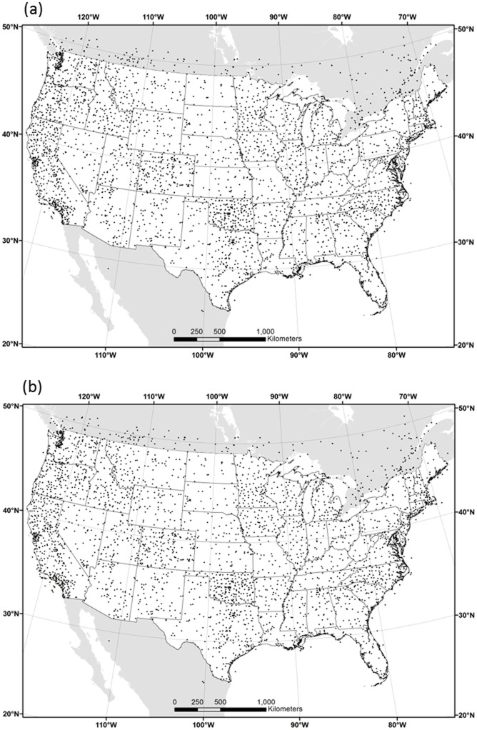
Climate data sets were developed for the conterminous US at 30 arc-second resolution in geographic (latitude/longitude) coordinates (Fig 1). A 30-arc-second grid cell is approximately 900 x 700 m at 40N latitude, and is referred to here as “800 m.” The boundaries of the grid are 22°N and 50°N and 65°W and 125°W, which are exactly coincident with other 800-m grids from the PRISM Climate Group [8]. The interpolation was performed separately in three overlapping regions: western, central and eastern US, and the resulting grids merged to form a complete conterminous US grid. The western region extends from the Pacific Coast to eastern Colorado, central from central Colorado to Lake Michigan, and eastern from eastern Minnesota to the eastern seaboard.

Fig 1. Map of study area and station locations.

Conterminous US and border area monthly average (a) mean dew point (T _dmean) stations and (b) minimum and maximum vapor pressure deficit (VPD _min and VPD _max) stations.

Care was taken to include as many islands offshore the US mainland as possible, but undoubtedly some very small islands were missed. To accommodate GIS shoreline data sets of varying quality and resolution, the modeling region was extended offshore several km and generalized to include bays and inlets. However, the gridded climate estimates are valid over land areas only.

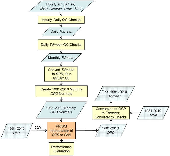
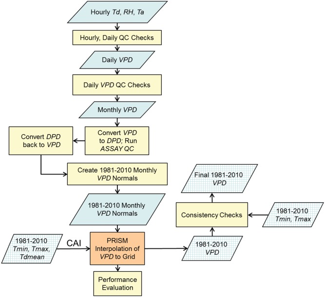
Overviews of the data processing and mapping work flows for T _dmean and for VPD _min and VPD _max are diagrammed in Figs 2 and 3, respectively. The process began with hourly and daily data for T _dmean, and hourly data for VPD _min and VPD _max, which were averaged to daily, and then monthly, time steps, with quality screening done at each stage (see Station Data and Processing section). At the monthly time step, all three variables were expressed as dew point depression (DPD) to take advantage of a spatial consistency quality control (QC) method using a version of PRISM called ASSAY (see Quality Control and Calculation of Monthly Values section). T _dmean was kept in the form of DPD for interpolation by PRISM, and converted back to T _dmean as a grid post-processing step. VPD _min and VPD _max were converted from DPD back to their original forms before interpolation by PRISM (see Mapping Methods section). A performance evaluation was conducted on the PRISM interpolation process (see Uncertainty Analysis section). As a final step, output grids from PRISM were checked for consistency with previously-created grids of 1981–2010 T _max and T _min.

Fig 2. Work flow diagram for data processing and mapping of T _dmean.

Cross-hatched boxes represent gridded data. See text for abbreviation definitions.

Fig 3. Work flow diagram for data processing and mapping of VPD _min and VPD _max.

VPD refers to either VPD _min or VPD _max. Cross-hatched boxes represent gridded data. See text for abbreviation definitions.

Station Data and Processing

Data Sources

Data from surface stations, numbering about 4,000 for T _dmean (44 km average station spacing) and 3,500 for VPD _max and VPD _min (47 km average station spacing) were obtained from a variety of sources (Table 1; Fig 1). Data from the National Weather Service (NWS) Automated Surface Observing System (ASOS) came via Unidata's Internet Data Distribution system and the National Climatic Data Center (NCDC) Integrated Surface Hourly/Integrated Surface Data archives (ftp://ftp.ncdc.noaa.gov/pub/data/noaa/), supplemented by the Solar And Meteorological Observation Network (SAMSON) and Integrated Surface Weather Observations CD-ROMs. NWS Cooperative Observer Program (COOP) and Weather Bureau Army Navy (WBAN) data were obtained from (http://www.ncdc.noaa.gov/cdo-web/). USDA Forest Service and Bureau of Land Management Remote Automatic Weather Station (RAWS) data came from archives at the Western Regional Climate Center (http://www.raws.dri.edu), the Real-time Observation Monitor and Analysis Network http://raws.wrh.noaa.gov), and from the MesoWest Local Data Manager (LDM) feed and website (http://mesowest.utah.edu/data). USDA Natural Resources Conservation Service (NRCS) Soil Climate Analysis Network (SCAN) observations were provided through the National Water and Climate Center web service (http://www.wcc.nrcs.usda.gov). Bureau of Reclamation AgriMet (AGRIMET) data were obtained from the Pacific Northwest Region (http://www.usbr.gov/pn/agrimet/), Great Plains Region (http://www.usbr.gov/gp/agrimet/), Upper Colorado Region in cooperation with the Utah Climate Center (https://climate.usurf.usu.edu/agweather.php), and Mid Pacific Region in cooperation with the Desert Research Institute (http://nicenet.dri.edu/) and the National Oceanic and Atmospheric Administration NOAA Idaho National Laboratory Weather Center (http://niwc.noaa.inel.gov/). Data were also collected from the Oklahoma Climatological Survey Mesonet (OKMESONET; http://www.mesonet.org/data/public/mesonet/mts), Colorado State University’s Colorado Agricultural Meteorological Network (COAGMET; http://ccc.atmos.colostate.edu/~coagmet), and a small number of miscellaneous stations from state and local networks.

Table 1. Source, averaging interval, and number of stations used in the mapping process.

Source	Averaging Interval	Stations Contributing ≥ 1 Month to Grids		Stations Contributing All 12 Months to Grids
		T dmean	VPD min VPD max	T dmean	VPD min VPD max
ASOS	Hourly	1960	1947	1789	1619
RAWS	Hourly	1066	1067	885	682
COOP	Daily	388	0	334	0
OKMESONET	Hourly	129	129	123	122
SCAN	Hourly	116	116	87	76
AGRIMET	Hourly	73	73	70	55
NDBC	Hourly	72	72	53	56
COAGMET	Hourly	63	63	54	50
WBAN	Daily	42	0	38	0
Other Networks	Daily	23	0	23	0
Total Surface Stations		4001	3467	3456	2660
NCAR/NCEP (Upper-air) Grid Points	1981–2010 monthly mean	69 a	69 a	69 a	69 a

^a Count for upper air is the number of grid points used.

To improve marine representation, data were obtained from coastal stations and offshore buoys operated by the NOAA National Data Buoy Center (NDBC; http://www.ndbc.noaa.gov/data/historical/stdmet). To better define humidity profiles at high elevations, mean monthly upper-air temperature, geopotential height, and relative humidity grid points for the western and eastern United States were obtained at 2.5-degree resolution for the period 1981–2010 from the National Center for Environmental Prediction (NCEP) Global Reanalysis (ftp://ftp.cdc.noaa.gov/Datasets/ncep.reanalysis.derived/pressure). The 5650-m level (~500 hPa) was chosen for the western US, and the 3050-m level (~700 hPa) for the eastern US. (Upper-air data were not needed in the central US, because of a lack of elevated terrain.) These levels were sufficiently far above the highest terrain features to minimize potential errors involved in estimating surface humidity statistics from free air values.

Quality Control and Calculation of Monthly Values

As shown in Table 1, station data were available at either an hourly or daily time step. Daily data were sufficient for T _dmean, but hourly data were required to calculate VPD _min and VPD _max. In some cases, hourly data were provided in the form of RH directly from the instrument. Range checks were performed to screen out values that were either impossible or could cause instabilities in the calculation of related statistics. If RH ≤ 0 or RH > 105, the value was set to missing. Otherwise, if RH < 0.5, it was set to 0.5, and if 100 < RH ≤ 105 (as sometimes occurs under saturated conditions), it was set to 100.

Dew point (T _d) was derived from hourly RH (%) and ambient temperature (T _a,°C) by calculating the saturation vapor pressure at T _a (SATVP _a) ([26], Eq 21):

$$SATV{P}_a=6.1094e^{\left(\frac{17.625T_a}{243.04+T_a}\right)}$$ (1)

and finding T _d (°C) [27]:

$$T_d=\frac{237.3\text{ln}\left[SATV{P}_a\left(\frac{RH}{611}\right)\right]}{7.5\text{ln}10-\text{ln}\left[SATV{P}_a\left(\frac{RH}{611}\right)\right]}$$ (2)

A consistency check was done to ensure that the calculated T _d was less than T _a; if not, each was set to missing.

As a range check, T _d values that fell below -68°C, or exceeded the statewide extreme maximum temperature record (http://www.ncdc.noaa.gov/extremes/scec/records) were set to missing. In addition, the hourly T _d values were subjected to a step check in which each value could not differ from that of the previous hour by more than 10°C; otherwise the current hour’s T _d was set to missing.

Hourly VPDs were calculated from a combination of T _a and T _d or T _a and RH, depending on which was available. If RH was available, VPD was calculated by: (1) finding SATVP _a from Eq 1; (2) finding the saturation vapor pressure at the previously calculated T _d:

$$SATV{P}_d=6.1094e^{\left(\frac{17.625T_d}{243.04+T_d}\right)}$$ (3)

and; (3) calculating VPD as

$$VPD=SATV{P}_a-SATV{P}_d$$ (4)

If T _d was available, VPD was obtained by calculating SATVP _d from Eq 3 and VPD from Eq 4. Each hourly VPD was subjected to a range check, where if VPD > 200 hPa or < 0 hPa, or if VPD ≥ SATVP _a, the value was set to missing.

Three persistence tests were done on T _a and T _d hourly values for each 24-hour period. If the maximum difference between any pair of hourly observations or the difference between the maximum and minimum value over the 24-hour period was less than 0.1°C, or the standard deviation of all values in the 24-hour period was less than 0.1°C, the day was considered a “flat day” and all variables, including the VPDs, were set to missing.

For networks with hourly data, T _dmean values were calculated by averaging available hourly observations, subject to the requirement that at least 18 of 24 observations be non-missing; fewer than 18 non-missing hourly observations resulted in a missing daily value. Daily VPD _min and VPD _max, as well as T _min, and T _max, were determined by finding the minimum and maximum hourly value, respectively, subject to the same data completeness requirement.

Daily maximum and minimum T _d (T _dmax, T _dmin) and mean T _a (T _mean) values were calculated for diagnostic purposes. Consistency checks were performed on daily combinations of T _dmean and temperature as follows: If T _max < T _dmax, T _min < T _dmin, or T _mean < T _dmean, all variables, including VPD _min and VPD _max, were set to missing.

The daily values were averaged to create monthly mean T _dmean, VPD _min, and VPD _max for each year of record. A minimum of 85% of non-missing daily values were required for a monthly value to be non-missing [28], [29].

The monthly averages were tested for spatial consistency using the ASSAY QC (quality control) system. ASSAY is a version of PRISM that estimates station values in their absence and compares them to the observed values, a procedure termed cross-validation [8]. The interpolation procedures in ASSAY are exactly the same as in PRISM; the only difference is that ASSAY interpolates to point (station) locations, rather than grid cells. As a rule, a large discrepancy between an observed station value and the interpolated estimate from ASSAY suggests that the station value is unusual compared to nearby stations, and may therefore be erroneous. In previous work, an ASSAY QC analysis was performed for T _dmean, with T _dmean expressed in the form of dew point depression (DPD) with T _min; that is, DPD = T _min−T _dmean. (As will be discussed in the next section, the DPD form of T _dmean was the favored method of expressing T _dmean for interpolation in this study.) In the previous ASSAY analysis of DPD, QC was done manually by trained personnel, and compared with the ASSAY results. It was found that when the absolute difference between the observation and ASSAY estimate of DPD exceeded 4.5°C, the value was considered erroneous by the manual method. Based on these results, in this study ASSAY QC was applied to T _dmean expressed as DPD, and station values producing absolute differences between the observation and estimate of more than 4.5°C were flagged as bad and set to missing. Overall, 0.8 percent of the monthly T _dmean values were set to missing using this method.

To take advantage of the ASSAY QC screening method, VPD _min and VPD _max were also expressed as DPD with T _min, termed DPD(VPD _min) and DPD(VPD _max), respectively. This involved: (1) calculating the saturation vapor pressure for the station’s T _min value (SATVP _a) using Eq 1; (2) subtracting the VPD from this value to get SATVP _d; (3) obtaining T _d from Eq 2, substituting SATVP _d for SATVP _a and using 100 for the RH value; and (4) subtracting the resulting T _d from T _min to obtain the DPD. Manual QC checks found that the same threshold of 4.5°C used in QC’ing DPD was suitable for DPD(VPD _min) and DPD(VPD _max) as well, and those exceeding this threshold were flagged as bad and set to missing. Overall, 0.7 percent of the monthly VPD _min values and 1.8 percent of the monthly VPD _max values were set to missing using this method.

Monthly values of T _dmean, VPD _min, and VPD _max passing the ASSAY QC screening were averaged over their period of record (POR), or 1981–2010, if available. A 1981–2010 monthly mean calculated using data from at least 23 of these 30 years (75% data coverage) was considered to be sufficiently characteristic of the 1981–2010 period, and was termed a “long-term” station. However, many stations had a POR of fewer than 23 years. Averages from stations with short PORs were subjected to adjustment to minimize temporal biases, as described in [8], Appendix A.

Mapping Methods

Mapping of 1981–2010 mean monthly T _dmean, VPD _min, and VPD _max was performed using PRISM [6–8], [30]. For each grid cell, PRISM calculated a local linear regression function between the atmospheric moisture variable and a predictor grid (see Climatologically-Aided Interpolation below). Nearby stations entering the regression were assigned weights based primarily on the physiographic similarity of the station to the grid cell. Physiographic factors relevant to this study were distance, elevation, coastal proximity, vertical atmospheric layer, and topographic position (relative to surrounding terrain). Detailed descriptions of the PRISM model algorithms, structure, input grids, and operation are given in [7], [8], and [30]. Details on the specific modeling approach for this study are given below.

Derive or Interpolate VPDmin and VPDmax?

Given that T _dmean is a basic atmospheric moisture variable from which other variables can be derived, early in this study the question was asked: do VPD _min and VPD _max need to be interpolated separately, or can they be derived from a combination of the T _dmean grid and previously-created grids of T _max and T _min? More specifically, can T _dmean be combined with T _max to estimate VPD _max and T _dmean combined with T _min to estimate VPD _min? To do this, we must assume that T _d = T _dmean and T _a = T _max at the time of VPD _max, and T _d = T _dmean and T _a = T _min at the time of VPD _min. To test these assumptions, monthly averages of VPD _min and VPD _max, as well as VPD _min and VPD _max estimated as described above, were calculated and averaged for each month over the ten-year period 2003–2012 at 100 randomly selected ASOS stations with hourly data. Results of this exercise are given in Table 2 for January and July, which bracket the range of monthly values observed during the year.

Table 2. Monthly averages of actual and estimated vapor pressure deficit.

2003–2012 January and July averages from 100 randomly-selected ASOS stations. Actual and estimated VPD values are expressed as 5^th percentile / mean / 95^th percentile.

VPD (hPa)	January	July
VPD min	0.2 / 0.8 / 1.6	0.9 / 3.3 / 9.7
Estimated VPD min	-0.6 / 0.7 / 1.6	-0.1 / 4.2 / 11.2
VPD max	1.5 / 5.9 / 12.3	15.2 / 26.9 / 47.7
Estimated VPD max	1.8 / 6.3 / 12.1	14.7 / 26.3 / 45.4

In Table 2, actual and estimated VPD _min and VPD _max are expressed as means and percentiles (5^th percentile / mean / 95^th percentile) so that the full distribution of values can be evaluated. Differences between actual and estimated VPD _max were generally within about three hPa or five percent across the distributions in both winter and summer. However, a proportion of the estimated VPD _min values fell below zero, which is not physically possible. This problem was most serious during winter; in January, a VPD _min of less than zero was estimated at 47 of the 100 stations. In these cases, T _dmean exceeded T _min, resulting in a negative VPD. In reality, the opposite was true, resulting in a positive VPD _min. Given this issue, deriving VPD _min and VPD _max from T _dmean, T _min, and T _max was not considered a viable option, leading us to interpolate VPD _min and VPD _max directly from station data.

Climatologically-Aided Interpolation

In previous work, constructing the 1971–2000 and 1981–2010 monthly normals for T _min and T _max used a DEM as the predictor grid (see [8] for details on methods used for mapping T _min and T _max). There were nearly 10,000 stations used in the mapping of the 1971–2000 T _min and T _max normals, and over 16,000 stations used in the 1981–2010 normals. In contrast, there were only 3,500–4,000 stations available for this study, with poor representation at high elevations. Faced with limited station data, we opted for the CAI method of interpolation. CAI uses an existing climate grid to improve the interpolation of another climate element for which data may be sparse or intermittent in time [31–36]. This method relies on the assumption that local spatial patterns of the climate element being interpolated closely resemble those of the existing climate grid (called the predictor grid). Uses of CAI fall into two main categories: (1) using a long-term mean grid of a climate element to aid the interpolation of the same element over different (usually shorter) averaging periods; and (2) using a grid of a climate variable to aid the interpolation of a different, but related, climate variable, such as interpolating annual extreme minimum temperature using January mean minimum temperature as the predictor grid [37]. A classic example of the first strategy involves mapping a long-term mean climatology carefully with sophisticated methods, then developing time series grids for shorter averaging periods (monthly or daily) using simpler and faster methods such as inverse-distance weighting to interpolate deviations from the mean climatology to a grid. These deviations can then be added to (e.g., temperature) or multiplied by (e.g., precipitation) the mean climatology to obtain the new grid.

Our use of CAI for this study falls into the second strategy, for which we use pre-existing grids of 1981–2010 mean monthly T _min and T _max as predictor grids in the interpolation process. A series of tests was conducted with ASSAY and PRISM to determine which of the 1981–2010 mean monthly T _min and T _max grids were the strongest predictors of the spatial patterns of T _dmean. T _min was found to be a good predictor, which is not surprising given that temperatures often reach the dew point at the time of T _min over much of the US. However, inspection of the interpolated grids revealed that in some areas subject to locally low temperatures, such as cold air pools in mountain valleys, the interpolated T _dmean exceeded the mean temperature, meaning that long-term mean RH exceeded 100 percent, which was not acceptable. In order to more closely tie the patterns of T _dmean to the patterns of the existing monthly T _min grids and their relatively large supporting station data sets, each T _dmean station value was expressed as the deviation from T _min, or DPD (T _dmean— T _min). Thus, in the interpolation process, PRISM was run with the 1981–2010 mean monthly T _min grid as the independent variable and DPD as the dependent variable. The local regression functions were generally not as strong as they were in the case of T _dmean vs. T _min, because DPD was essentially the residual from the T _dmean vs. T _min relationship. Once the mean monthly DPD values were mapped in this manner, the final T _dmean grid was obtained by adding the DPD grid to the 1981–2010 T _min grid. The result was an interpolated T _dmean grid that was highly consistent in an absolute, as well as relative sense, with the associated T _min grid. An example of the relationship between 1981–2010 January mean observed DPD and gridded T _min for a location north of the Wind River Mountains of Wyoming (43.6N, 109.73W) is shown in Fig 4a. This area is characterized by persistent wintertime cold air pools in mountain valleys, where the humidity is high and T _min is less than T _dmean (DPD<0). Above these cold pools, T _min increases and rises above T _dmean (DPD>0).

Fig 4. Scatterplots of relationships between predictor grid and interpolated variables.

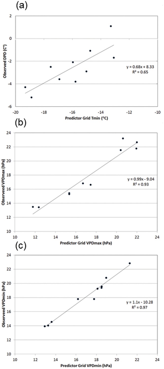
1981–2010 mean monthly (a) dew point depression (DPD) vs. minimum temperature (T _min) for January in western Wyoming; (b) minimum vapor pressure deficit (VPD _min) vs. first-guess VPD _min for June near Las Vegas; and (c) maximum vapor pressure deficit (VPD _max) vs. first-guess VPD _max for October in San Francisco.

An additional series of tests was conducted with PRISM and ASSAY to determine whether either of the pre-existing 1981–2010 mean monthly T _min and T _max grids could be used as predictors of the spatial patterns of VPD _min and VPD _max. T _max was found to be a good predictor of VPD _max; and the same was true for T _min and VPD _min. However, once T _dmean was mapped, a superior, second-generation CAI method using T _dmean became available. Termed CAI2, this method involves using the result of a CAI interpolation as the predictor grid in another CAI interpolation. Specifically, a first-guess VPD _min grid was created by calculating the VPD associated with the combination of the T _dmean and T _min grids using Eqs 1, 3 and 4. Similarly, a first-guess VPD _max grid was found by calculating the VPD associated with the combination of the T _dmean and T _max grids. These “first-guess” predictor grids represented what the VPD _min and VPD _max spatial patterns would be like if T _d was held constant throughout the day at T _dmean, and VPD _min occurred at the time of T _min and VPD _max occurred at the time of T _max. While these assumptions are not always correct (see Table 2), they are sufficiently reasonable to produce predictor grids that closely match the relative spatial patterns of VPD _min and VPD _max.

An example of the relationship between 1981–2010 June mean observed VPD _min and first-guess predictor grid VPD _min for a location near Las Vegas, Nevada (35.79N, 115.26W) is shown in Fig 4b. In this desert environment, VPD _min is still relatively large (14–22 hPa), even at its minimum for an average day in June. The lowest VPD _min values are found at higher elevations, where temperatures are cooler. An example of the relationship between 1981–2010 October mean observed VPD _max and the first-guess predictor grid VPD _max for a location in San Francisco, along the California coastline (37.76N, 122.45W), is shown in Fig 4c. In this case, the lowest VPD _max values are found along the immediate coast where temperatures are cooler and moisture is greater, with higher values in warmer and drier inland areas.

PRISM Weighting Functions

During PRISM interpolation, upon entering the local linear regression function for a pixel, each station was assigned a weight based on several factors. The combined weight (W) of a station is given by the following:

$$W=W_c{\left[F_d{W}_d{}^2+F_z{W}_z{}^2\right]}^{1/2}{W}_p{W}_l{W}_t$$ (5)

where W _c, W _d, W _z, W _p, W _l, and W _t are cluster, distance, elevation, coastal proximity, vertical layer, and topographic position weights, respectively, and F _d and F _z are user-specified distance and elevation weighting importance scalars [8], [38]. All weights and importance factors, individually and combined, are normalized to sum to unity. PRISM weighting functions not enabled in this study were topographic facet weighting, which is used primarily to identify rain shadows in precipitation mapping, and effective terrain height weighting, which identifies orographic precipitation regimes based on terrain profiles [8].

Table 3 summarizes how the PRISM climate regression and station weighting functions accounted for physiographic climate forcing factors, and provides citations for further information. Cluster weighting was used to keep clusters of stations that represent similar local conditions from dominating the regression functions; both horizontal and vertical separations were considered [8]. Distance and elevation weighting were used to accommodate the spatial coherence of climatic regimes, both horizontally and vertically [8].

Table 3. PRISM weighting algorithms and associated physiographic climate forcing factors.

Inputs to the algorithms and references on their formulation and use are included. Methods used to prepare the gridded model inputs are summarized in [8], Tables 1 and 2.

PRISM Algorithm	Description	Physiographic Forcing Factors	Inputs to Algorithm	Reference
Climate Regression Function (CAI)	Develops local relationships between a climate predictor grid and the interpolated variable	Incorporates physiographic features implicit in the climate predictor grid	Station data; climate predictor grid	This paper, Mapping Methods Section; [37] Section 4b
Cluster Weighting	Downweights stations clustered with others	--	Station locations and elevations	[8], Appendix B
Distance Weighting	Upweights stations that are horizontally close	Horizontal coherence of climate regimes	Station locations	[8], Section 4.2.1
Elevation Weighting	Upweights stations that are vertically close	Vertical coherence of climate regimes	DEM; station locations and elevations	[7], Section 4.1
Coastal Proximity Weighting	Upweights stations having similar exposure to coastal influences	Effects of water bodies on temperature and moisture	DEM; coastal proximity grid; station locations	[7], Section 6; [30] Section 2.3.2; [8] Section 4.2.2
Two-Layer Atmosphere Weighting	If an inversion is present, upweights stations in the same vertical layer (boundary layer or free atmosphere)	Temperature inversions; vertical limit to moist boundary layer (humidity)	DEM; inversion height grid; station locations	[7], Section 7; [30], Section 2.3.4
Topographic Position Weighting	Upweights stations having similar heights above the local terrain	Cold air drainage and pooling in topographic depressions	DEM; topographic index grid; station locations	[38], Section 4; [8], Section 4.2.5

Coastal proximity weighting accounted for sharp gradients in temperature and atmospheric moisture from coastlines to interior regions [7], [8], [30]. Atmospheric layer weighting was useful where temperature inversions occurred, by delineating gradients in the relationship between temperature and atmospheric moisture along the transition from the relatively humid boundary layer near the earth’s surface to the drier free atmosphere above [7], [30]. Topographic position weighting differentiated topographically sheltered locations where cold, moist air may accumulate, from more exposed locations not susceptible to cold air pooling, such as hill slopes and ridge tops [8], [38].

Relevant PRISM control parameters are listed in Table 4. A minimum of 25 stations were required for each pixel’s regression function, and the radius of influence was expanded from a minimum of 20 km to as far as necessary to reach the 25-station threshold. T _dmean slope bounds were expressed as the change in DPD per unit T _min from the predictor grid, and VPD slopes expressed as the change in VPD per unit first-guess VPD from the predictor grid. The maximum and minimum allowable regression slopes were derived from test runs of PRISM where distributions of slope values were created and outliers examined to determine validity, combined with performance assessments using ASSAY. In the final PRISM interpolation runs, slopes falling outside the designated bounds were set to values that fell halfway between the default slope and the bound that the slope violated (either the maximum or minimum). In the western region, allowable slopes in the relationship between VPD _max and the first-guess VPD _max were constrained to fall between 0.99 and 1.01, so as to avoid a rare circumstance of predicting a VPD _max that might approach the value of SATVP _a at T _max (hence producing a very low RH) in the warmest and driest areas. The exponential relationship between temperature and SATVP _a steepens at higher temperatures, leaving less room for error in extremely low-humidity situations. Unconstrained, the average slope of the 5.5 million PRISM regression functions (one per pixel) for July (the warmest month) across the western region was 1.017, with the 10th percentile at 0.964 and the 90th at 1.15, so this constraint had a very slight effect.

Table 4. Values of relevant PRISM interpolation parameters.

Regression slope bounds are sometimes different among regions; values separated by forward slashes are for west, central, and east regions, respectively. See [7] and [8] for details on PRISM parameters and Table 3 for citations to details on weighting function formulations.

Name	Description	T dmean	VPD min	VPD max
Regression Function
R	Radius of influence	20 km*	20 km*	20 km*
s t	Minimum number of total stations desired in regression	25 stations	25 stations	25 stations
β 1ma	Min valid regression slope, layer 1	-0.5 +	-10/-1/-1.5 #	0.99/0/0 #
β 1xa	Max valid regression slope, layer 1	2.5 +	10/2/1 #	1.01/1.5/1.5
β 1da	Default regression slope, layer 1	0.5 +	1/0.5/0.5 #	1/1/1 #
β 1mb	Min valid regression slope, layer 2	-0.5 +	-10/-1/-1 #	0.99/0/0 #
β 1xb	Max valid regression slope, layer 2	2.5 +	10/2/1 #	1.01/1.5/1.5 #
β 1db	Default regression slope, layer 2	0.5 +	1/1/0.5 #	1/1/1 #
Distance Weighting
A	Weighting exponent	1.5	1.5	1.5
F d	Importance factor	0.5	0.5	0.5
D m	Minimum allowable distance	0 km	0 km	0 km
Elevation Weighting
B	Weighting exponent	1.5	1.5	0.5
F z	Importance factor	0.5	0.5	0.5
Δz m	Station-grid cell elev difference below which weight is maximum	100 m	100 m	100 m
Δz x	Station-grid cell elev difference above which weight is zero	5000 m	5000 m	5000 m
Coastal Proximity Weighting
v	Weighting exponent	1.0	1.0	1.0
Δp m	Station-grid cell proximity difference below which weight is maximum	100 $	100 $	100 $
Δp x	Station-grid cell proximity difference above which weight is zero	300 $	300 $	300 $
Vertical Layer Weighting
y	Weighting exponent	0.5	0.5	0.5
Δl m	Station-grid cell distance to adjacent layer below which weight is maximum	100 m	100 m	100 m
Δl x	Station-grid cell distance to adjacent layer above which weight is zero	N/A	N/A	N/A
Topographic Position Weighting
μ	Weighting exponent	1.5	1.5	1.5
Δt m	Station-grid cell topo difference below which weight is maximum	50 m	50 m	50 m
Δt x	Station-grid cell topo difference above which weight is zero	900 m	900 m	900 m

* Expands as needed to encompass minimum number of total stations desired in regression (s _t).

⁺ Slope is expressed as the change in dew point depression (DPD) per unit Tmin from the predictor grid

^# Slope is expressed as the change in VPD per unit first-guess VPD from the predictor grid

^$ Units are effective distance in grid cells from the coast, incorporating terrain barriers

Station weighting parameters were very similar among the three variables, and were generally set to the same values across the three regions. The exception was the elevation weighting exponent for VPD _max, which was set to 0.5, compared to 1.5 for the other variables. T _max and VPD _max occur primarily during the day, when the atmosphere is more likely to be well-mixed, and vertical gradients in atmospheric moisture more slowly varying. As a rule, the weighting exponents were set to the lowest values possible to achieve the desired effects. Being parsimonious with the weighting exponents ensured that the station data entering the local regression functions were not down-weighted unnecessarily, which can weaken the statistical results by decreasing the effective number of stations in the regression.

A number of small but noticeable inconsistencies in DPD values between adjacent stations were observed during the summer months in some agricultural areas, most notably in eastern Colorado. Further investigation revealed that relatively low DPD values were coming from two networks: AGRIMET and COAGMET. Stations in these networks are typically sited in or near irrigated fields for use in water management calculations, resulting in more humid conditions than locations away from irrigated areas. Given that the data from these networks were of otherwise high quality, it was unreasonable to simply omit these two networks outright. This issue raised questions about whether the grids should, or could, represent conditions over irrigated land. Concerns over attempting to do so are summarized as follows:

1. Siting requirements for these station networks state that the station must be located in, or immediately adjacent to, an irrigated field to be representative of an irrigated environment. This suggests that the effects of irrigation on humidity are highly local, and which may not extend beyond one 800-pixel. In practice, however, these stations influenced the interpolated estimates many km away, well beyond the likely limits of irrigation in many instances.

2. A complete picture of the location and extent of irrigated lands across the country was unavailable; further, there was no interpolation mechanism in place to constrain the influence of stations on irrigated fields to just those lands. It was also unclear how to modify DPD values in the many irrigated areas not represented by station data.

3. We, and likely others, will be using these atmospheric moisture climatologies as the predictor grids for CAI mapping of monthly and daily time series of the same variables. Given that many of these time series will extend back a century or more, when crop patterns and irrigation practices were very different than today, patterns of humidity caused by today’s irrigation patterns could be propagated to times when they are not applicable.

Given these concerns, a subjective middle ground was taken, where a few (<10) stations causing the most severe spatial discrepancies were omitted from the T _dmean dataset, and the rest retained. For consistency, the same stations were also omitted from the VPD _min and VPD _max datasets.

Grid Post-processing

Once monthly grids of T _dmean, VPD _min, and VPD _max were generated with PRISM, post-processing checks were made to ensure that the interpolated values did not exceed reasonable ranges, and that consistency was maintained among the three variables and with the pre-existing 1981–2010 mean monthly T _min and T _max grids. Given that the 1981–2010 monthly means are by definition made up of yearly values above and below these means, the acceptable ranges were defined to be more restrictive than what would be allowed on, say, a single day. If T _dmean > (T _mean− 0.5°C), T _dmean mean was set equal to T _mean− 0.5°C. If VPD _min < 0.01 hPa, VPD _min was set equal to 0.01 hPa. If VPD _min < 0.001 SATVP _a at T _min (i.e., RH > 99.9%), VPD _min was set equal to 0.001 SATVP _a at T _min. If VPD _max > 0.95 SATVP _a at T _max (i.e., RH < 5%), VPD _max was set equal to 0.95 SATVP _a at T _max. The number of grid cells affected by these restrictions was limited to a handful in remote mountainous regions of the western US.

Results and Discussion

Spatial Patterns

Dew Point

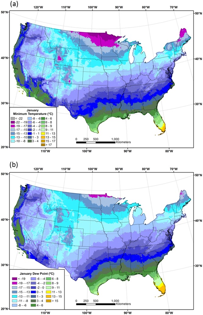
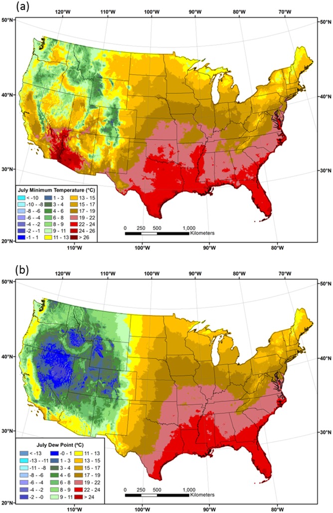
Maps of 1981–2010 mean T _min and T _dmean in January and July are shown in Figs 5 and 6, respectively. The general patterns of T _dmean are similar to those of T _min, especially in winter. In January, values are lowest in the northern tier of states, and in cold pools along valley bottoms in the West (Fig 5). T _dmean is high in the eastern part of the country in July, exceeding 20°C in much of the Southeast, which is exposed to the transport of moist air from the Gulf of Mexico (Fig 6). Despite relatively warm temperatures, July T _dmean is low in the dry Intermountain West. A notable exception is the Southwest, where the summer monsoon produces locally elevated T _dmean values.

Fig 5. Maps of January minimum temperature and dew point.

Conterminous US 1981–2010 mean January (a) minimum temperature (T _min) and (b) dew point temperature (T _dmean).

Fig 6. Maps of July minimum temperature and dew point.

Conterminous US 1981–2010 mean July (a) minimum temperature (T _min) and (b) dew point temperature (T _dmean).

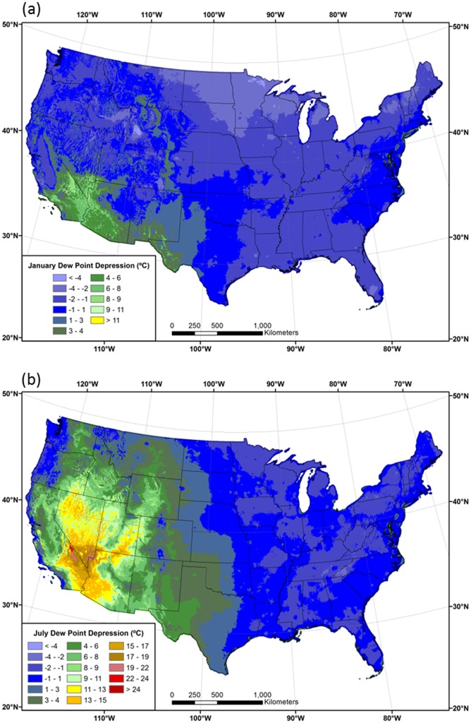
Interpolated DPDs between T _min and T _dmean (T _min—T _dmean) for January and July are shown in Fig 7. DPD is the original variable interpolated with PRISM before being added to the T _min grid to obtain T _dmean. In January, DPDs are mostly near zero or negative, meaning that T _dmean is similar to, or greater than, T _min over much of the country. In the northern US and in persistent cold pools in large inland valleys of the West, T _dmean is as much as 3–5°C greater than T _min (Fig 7a). For example, the 1981–2010 mean January T _dmean at the International Falls, MN ASOS station is -18.1°C and the mean January T _min is -21.3°C. In contrast, T _dmean averages 6–8°C lower than T _min in the southwestern US, which is a testament to the region’s aridity, even in winter.

Fig 7. Maps of dew point depression (DPD).

Conterminous US difference between the 1981–2010 mean minimum temperature and the 1981–2010 mean dew point temperature (T _min—T _dmean) for (a) January and (b) July.

In July, T _dmean and T _min have similar values in the eastern half of the country. Interestingly, major metropolitan areas such as St. Louis, Kansas City, Minneapolis, and Detroit, and several eastern seaboard cities, are visible as small areas of relatively warm T _min values, resulting in positive differences between T _min and T _dmean of 1–3°C (dark green spots in Fig 7b). The West is dominated by larger positive differences, where T _min is much higher than T _dmean. The changeover from near-zero to positive differences roughly follows the 100^th meridian. Notable exceptions are the West Coast, where cool, marine air penetrates inland, and areas of the Southwest affected by the summer monsoon. The core area of maximum DPD is centered on southeastern California, Nevada, western Arizona, and lower elevations of Utah, where T _dmean averages 10–25°C lower than T _min. A combination of low moisture content (low T _dmean) and limited time for nighttime cooling (high T _min) during summer contribute to these high DPDs. Methods that estimate T _dmean by assuming it is equal to T _min would experience the largest errors in this region [22].

Vapor Pressure Deficit

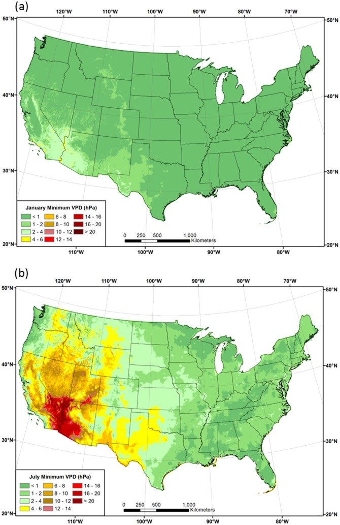
Patterns of 1981–2010 mean VPD _min in January and July are shown in Fig 8. In winter, VPD _min is low (<1 hPa) over most of the country, due to a combination of low temperatures and relatively small differences between T _a and T _d during the morning hours (Fig 8a). Vapor pressure varies exponentially with temperature; for example, a difference between T _a and T _d of 1°C amounts to a VPD of 0.15 hPa at 20°C, but less than 0.05 hPa at 0°C. In July, VPD _min is also low in the eastern US, but exceeds 5 hPa over much of the West, reaching maxima of over 20 hPa in the desert southwest (Fig 8b).

Fig 8. Maps of mean minimum vapor pressure deficit (VPD _min).

1981–2010 mean monthly VPD _min for (a) January and (b) July.

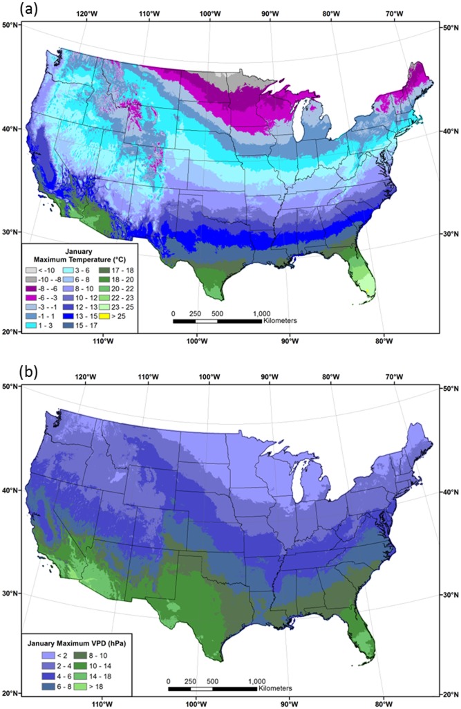
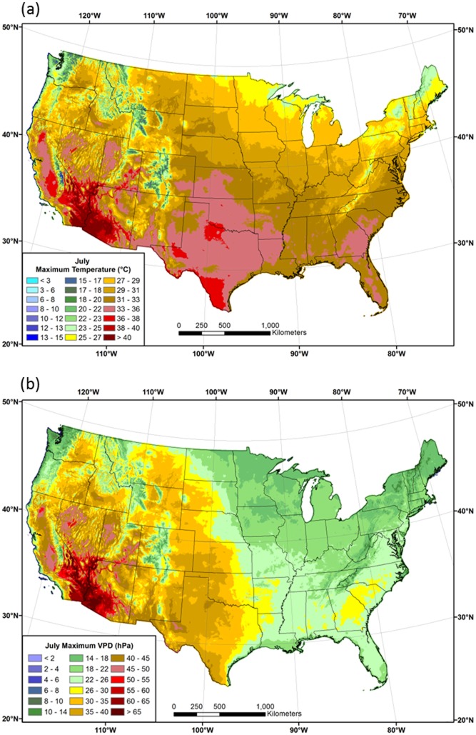
Spatial patterns of 1981–2010 mean T _max and VPD _max in January and July are shown in Figs 9 and 10, respectively. Patterns of VPD _max roughly follow those of T _max in January, with the lowest values in the northern tier and western mountains, and the highest in the southern states (Fig 9). In July, the area of high VPD _max expands considerably, exceeding 25 hPa over much of the western US, and reaching a maximum of over 60 hPa in the desert southwest (Fig 10). Coastal regions of the West exhibit relatively low VPD _max values, as they did for DPD. Similarly low values are found at higher elevations, illustrating the strong spatial relationship between VPD _max and T _max. In the east, VPD _max values in the Midwest and northeast are mostly less than 20 hPa, while those in the southeast can range above 25 hPa; a notable maximum occurs in the piedmont region of Georgia and the Carolinas.

Fig 9. Maps of January maximum temperature and vapor pressure deficit.

Conterminous US 1981–2010 mean January (a) maximum temperature (T _max) and (b) maximum vapor pressure deficit (VPD _max).

Fig 10. Maps of July maximum temperature and vapor pressure deficit.

Conterminous US 1981–2010 mean July (a) maximum temperature (T _max) and (b) maximum vapor pressure deficit (VPD _max).

Relative Humidity Derivation

RH can be derived from VPD and T _a by calculating SATVP _a at the desired temperature from Eq 1, and factoring in the appropriate VPD:

$$RH=100(SATV{P}_a-VPD)/SATV{P}_a$$ (6)

On a gridded basis, if only T _max and T _min are available to estimate T _a, and only VPD _min and VPD _max available to estimate VPD, grids of minimum RH (RH _min) can be approximated by substituting VPD _max for VPD and T _max for T _a, and maximum RH (RH _max) can be similarly derived using VPD _min and T _min. In performing these derivations, we make the assumption that T _a = T _min and VPD = VPD _min at the time of day when RH _max occurs, and T _a = T _max and VPD = VPD _max at the time of day when RH _min occurs. To evaluate the error introduced by these assumptions, we calculated 2003–2012 mean monthly RH _min and RH _max for the same 100 ASOS stations used in Table 2 and compared them with the estimated RH _min that would result from substituting VPD _max for VPD and T _max for T _a, and RH _max resulting from using VPD _min and T _min. As expected, T _max and VPD _max were slightly higher than T _a and VPD at the hour of RH _max, and T _min and VPD _min were slightly lower than T _a and VPD at the hour of RH _min (Table 5). As a result, the substitutions resulted in an overestimation of RH _min and an underestimation of RH _max. The differences averaged less than five percent in all months, suggesting that the derived grids are reasonable, but not exact, measures of the true RH.

Table 5. Results of temperature and vapor pressure deficit substitution in the derivation of minimum and maximum relative humidity.

2003–2012 January and July averages from 100 randomly-selected ASOS stations. Actual and estimated RH values are expressed as a distribution: 5^th percentile / mean / 95^th percentile.

Variable	January	July
T a at the hour of RH min (°C)	4.7	29.8
T max (°C)	6.2	30.2
VPD at the hour of RH min (hPa)	5.7	26.4
VPD max (hPa)	5.9	26.9
RH min (%)	19 / 44 / 64	14 / 39 / 55
Estimated RH min (%)	20 / 48 / 67	15 / 40 / 55
T a at the hour of RH max (°C)	-1.1	19.2
T min (°C)	-4.2	18.4
VPD at the hour of RH max (hPa)	0.8	3.4
VPD min (hPa)	0.8	3.3
RH max (%)	51 / 86 / 94	51 / 85 / 96
Estimated RH max (%)	50 / 85 / 93	50 / 85 / 96

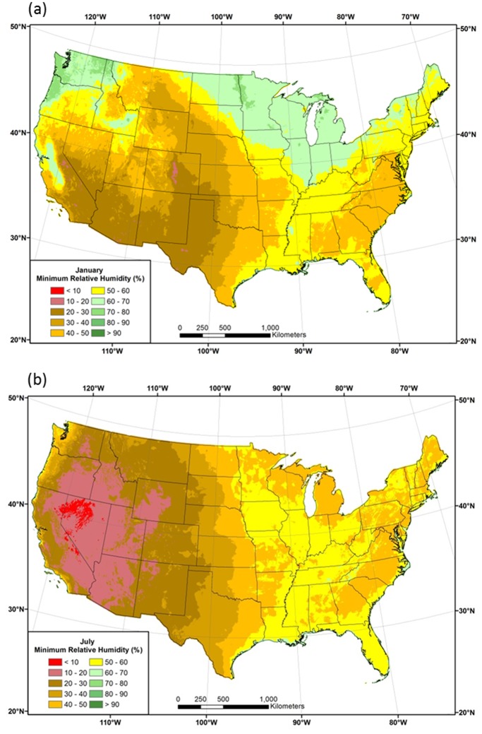
Maps of estimated 1981–2010 mean January and July RH _min, estimated from grid values of VPD _max and T _max, reveal some interesting features not easily seen in the maps of VPD _max (Fig 11). In January, RH _min values are as low as 10–15% on the lee side of the Rocky Mountains, associated with dry, Chinook (downslope) winds produced by a strong westerly jet stream. In contrast, RH _min values exceed 70% in the winter-wet Pacific Northwest. RH _min values are also above 70% in California’s Central Valley and Idaho’s Snake Plain, where extended periods of high pressure and calm winds promote temperature inversions that often result in persistent fog and low clouds (Fig 11a). Higher RH _min values in the upper Midwest reflect frequent cloudy weather during winter in this region.

Fig 11. Maps of minimum relative humidity.

Conterminous US 1981–2010 mean minimum relative humidity (RH _min) estimated from mean maximum temperature (T _max) and mean maximum vapor pressure deficit (VPD _max) for (a) January and (b) July.

RH _min patterns in July show a divided country, with a dry west and moist east (Fig 11b). The exception is the West Coast, where cool, moist onshore flow maintains relatively high humidity values throughout the day. The lowest RH _min (<10%) values are centered in Nevada, and more generally in the Great Basin. In the east, the highest values are found in regions that receive substantial moisture from the Gulf of Mexico, such as the southern Appalachians and Mississippi Valley.

Uncertainty Analysis

Estimating the true errors associated with spatial climate data sets is difficult, and subject to its own set of errors [36]. This is because the true climate field is unknown, except at a relatively small number of observed points, and even these are subject to measurement and siting uncertainties (as has already been noted in the case of irrigated land, for example). Leave-one-out cross validation (C-V) approach is the most common evaluation method where each station is omitted from the dataset one at a time, the station value estimated in its absence, and the estimate and observation compared. The mean absolute error (MAE) and bias are typically calculated once the process is complete. While this approach is commonly used to assess error in interpolation studies, and is reported here, there are several disadvantages. An obvious disadvantage is that no error information is provided for locations where there are no stations. The single-deletion method favors interpolation models that heavily smooth the results, so that deletion of one station is relatively unimportant to the stability of the estimate. Randomly withholding a larger percentage of the station data at once can help to minimize this issue, as well as provide more robust error statistics. Withholding a stratified sample from the analysis is useful in detecting specific weaknesses or issues in the interpolation, as was done to investigate irrigated stations (also, see [36] for an example).

In this study, uncertanties in the mapped estimates were initially estimated by performing a C-V exercise with ASSAY, and the results compiled for each month for each of the three modeling regions (west, central, and east).

Even accounting for weaknesses in the C-V methodology, these errors are underestimates of the actual C-V uncertainty. One overlooked aspect of CAI is that it relies on predictor grids which have their own interpolation errors. These errors accumulate from one CAI generation to the next. For T _dmean, uncertainties in the interpolated T _min predictor grids must be accounted for. In turn, VPD _min relies on interpolated T _min and T _dmean, and VPD _max relies on T _max, as well as T _min and T _dmean.

To quantify the effects of error propagation on the CAI MAEs, the predictor grid interpolation error was introduced at each CAI step by using ASSAY interpolated estimates at station locations in their absence instead of the predictor grid values, which already have those station values built in. For T _dmean, T _min values for all stations used in the mapping of the T _min predictor grid were estimated in their absence using ASSAY, and estimates common to both the T _min and T _dmean station datasets used as the values of T _min in an ASSAY C-V exercise for T _dmean. T _min values for stations used in the interpolation of T _dmean but not T _min, such as those from the SCAN and COAGMET networks, could not be estimated by ASSAY, because they were not used to create the predictor grid. However, they could still be included in the T _dmean C-V error estimation because, by definition, the estimates at their location on the T _min predictor grid were made in their absence.

For VPD _min, ASSAY estimates of station T _dmean values, predicted using ASSAY estimates of T _min as described above, were used in combination with ASSAY estimates of T _min to form station values of first-guess VPD _min, used as the predictor in the interpolation of VPD _min. The result was station values of first-guess VPD _min that accounted for errors in the interpolation of both T _min and T _dmean. These were used as the values of first-guess VPD _min in a C-V assessment of VPD _min with ASSAY. VPD _max involved the same steps as VPD _min, except that first-guess VPD _max values were formed from a combination of ASSAY estimates of T _max and T _dmean. Again, a C-V exercise for VPD _max was performed with ASSAY.

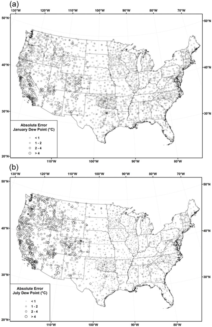
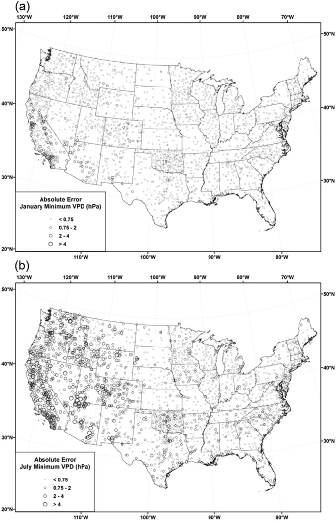
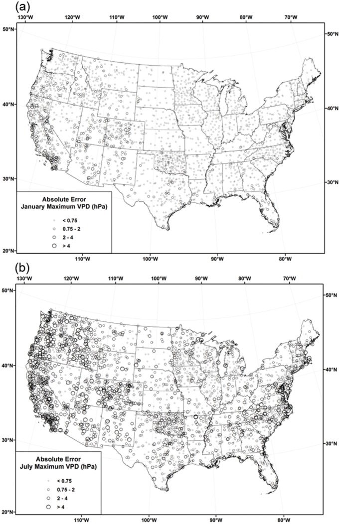
Table 6 reports monthly ASSAY cross-validation MAEs for each of the modeling regions. MAEs that account for CAI interpolation error propagation are denoted with a CAI or CAI2. Figs 12, 13 and 14 show the distribution of cross-validation absolute errors at stations across the country for T _dmean, VPD _min, and VPD _max, respectively.

Table 6. PRISM monthly cross-validation mean absolute errors (MAEs).

Both interpolation-only MAEs, and MAEs accounting for uncertainties in the predictor grids (denoted by CAI or CAI2), are given below. See text for details.

Region/Variable	Month
	Jan	Feb	Mar	Apr	May	Jun	Jul	Aug	Sep	Oct	Nov	Dec
West
T max (°C)	0.65	0.63	0.63	0.64	0.64	0.66	0.69	0.68	0.66	0.62	0.57	0.61
T min (°C)	0.98	0.93	0.85	0.82	0.87	0.97	1.08	1.09	1.11	1.04	0.95	0.96
T dmean (°C)	0.69	0.65	0.66	0.69	0.76	0.84	0.92	0.91	0.87	0.75	0.70	0.69
T dmean CAI (°C)	0.76	0.75	0.77	0.79	0.88	1.00	1.12	1.10	1.03	0.86	0.80	0.79
VPD min (hPa)	0.24	0.19	0.23	0.29	0.41	0.60	0.79	0.76	0.61	0.41	0.27	0.19
VPD min CAI2 (hPa)	0.31	0.28	0.36	0.45	0.65	0.89	1.25	1.17	0.99	0.64	0.41	0.28
VPD min (%)	41.9	31.2	32.2	31.0	28.5	30.1	30.5	32.1	32.2	29.2	34.0	33.7
VPD min CAI2 (%)	58.5	45.2	50.0	45.8	42.9	45.8	48.3	48.7	52.0	44.7	51.3	49.7
VPD max (hPa)	0.50	0.49	0.59	0.69	0.89	1.21	1.47	1.45	1.17	0.76	0.52	0.43
VPD max CAI2 (hPa)	0.57	0.58	0.70	0.82	1.10	1.46	1.86	1.81	1.43	0.97	0.63	0.52
VPD max (%)	11.1	8.7	7.4	6.4	6.1	6.3	6.0	5.9	5.8	5.8	7.6	10.1
VPD max CAI2 (%)	11.8	10.2	8.4	7.0	6.8	6.8	6.9	6.9	6.5	6.7	8.5	11.4
Central
T max (°C)	0.44	0.46	0.48	0.48	0.46	0.44	0.44	0.43	0.42	0.41	0.38	0.40
T min (°C)	0.65	0.63	0.55	0.55	0.53	0.53	0.55	0.58	0.63	0.67	0.64	0.63
T dmean (°C)	0.45	0.42	0.40	0.42	0.42	0.45	0.45	0.44	0.43	0.41	0.41	0.42
T dmean CAI (°C)	0.47	0.44	0.43	0.45	0.45	0.48	0.48	0.48	0.46	0.43	0.43	0.44
VPD min (hPa)	0.11	0.12	0.15	0.20	0.28	0.37	0.45	0.43	0.34	0.23	0.16	0.11
VPD min CAI2 (hPa)	0.13	0.15	0.19	0.27	0.37	0.49	0.60	0.56	0.46	0.32	0.21	0.15
VPD min (%)	22.4	22.0	20.3	19.3	22.8	23.6	29.6	33.0	31.3	28.4	23.3	23.2
VPD min CAI2 (%)	28.5	28.8	26.4	26.5	31.9	33.4	42.0	47.0	44.0	38.7	31.2	29.9
VPD max (hPa)	0.24	0.28	0.37	0.50	0.64	0.75	0.90	0.86	0.67	0.42	0.30	0.24
VPD max CAI2 (hPa)	0.29	0.34	0.43	0.62	0.79	0.96	1.13	1.07	0.84	0.55	0.37	0.30
VPD max (%)	5.3	5.1	4.2	3.8	3.9	3.6	3.8	3.7	3.5	3.2	3.7	5.1
VPD max CAI2 (%)	6.3	6.1	5.0	4.7	4.7	4.6	4.7	4.5	4.4	4.1	4.5	6.1
East
T max (°C)	0.40	0.46	0.49	0.51	0.50	0.49	0.48	0.47	0.43	0.42	0.37	0.37
T min (°C)	0.62	0.64	0.61	0.65	0.65	0.60	0.60	0.63	0.69	0.71	0.64	0.61
T dmean (°C)	0.46	0.42	0.40	0.40	0.40	0.40	0.38	0.38	0.40	0.39	0.39	0.39
T dmean CAI (°C)	0.46	0.43	0.42	0.43	0.42	0.42	0.41	0.41	0.44	0.42	0.41	0.40
VPD min (hPa)	0.10	0.12	0.19	0.25	0.31	0.36	0.38	0.38	0.33	0.24	0.18	0.13
VPD min CAI2 (hPa)	0.13	0.15	0.23	0.32	0.39	0.48	0.50	0.48	0.41	0.30	0.22	0.15
VPD min (%)	25.0	26.5	28.7	29.0	35.1	40.1	42.5	47.5	54.0	43.4	32.3	29.3
VPD min CAI2 (%)	33.2	33.9	36.7	40.1	51.9	63.7	77.8	78.9	78.9	64.4	42.8	38.1
VPD max (hPa)	0.25	0.28	0.50	0.59	0.75	0.93	1.01	0.91	0.73	0.48	0.34	0.26
VPD max CAI2 (hPa)	0.28	0.32	0.45	0.69	0.89	1.07	1.23	1.12	0.89	0.59	0.40	0.30
VPD max (%)	6.1	5.4	5.1	4.9	5.1	5.2	5.4	5.1	4.7	4.2	4.6	5.8
VPD max CAI2 (%)	6.6	5.7	5.5	5.6	5.9	6.1	6.6	6.3	5.9	5.1	5.2	6.3

Fig 12. Maps of T _dmean absolute cross-validation errors.

Errors for 1981–2010 mean monthly T _dmean in (a) January and (b) July.

Fig 13. Maps of VPD _min absolute cross-validation errors.

Errors for 1981–2010 mean monthly VPD _min in (a) January and (b) July.

Fig 14. Maps of VPD _max absolute cross-validation errors.

Errors for 1981–2010 mean monthly VPD _max in (a) January and (b) July.

Dew Point

In general, T _dmean interpolation errors in the west were greater than those in the central and eastern US, due primarily to terrain-induced complexities in the vertical distribution of moisture and temperature. This is evidenced by higher absolute errors in the Rocky Mountains, Cascades, and Sierra Nevada (Fig 12). Regionally, MAEs for T _dmean, interpolated as DPD (T _min−T _dmean), were less than 1°C in the west and less than 0.5°C in the central and east (Table 6). CAI MAEs that accounted for error propagation were 0.1–0.2°C larger than those that did not in the west, but less than 0.05°C larger in the central and east, owing to larger T _min interpolation errors in the west.

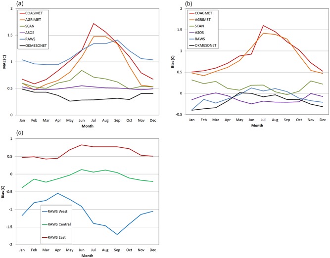
The T _dmean C-V analysis showed that the MAEs were inflated by systematic positive biases (lower observed DPD and higher T _dmean than predicted) in the COAGMET and AGRIMET networks. In fact, bias accounted for nearly all of the MAE. As discussed previously, stations in these networks were typically sited in or near irrigated fields for use in water management calculations. Despite subjective omission of stations producing the largest spatial inconsistencies, network-wide biases were still noticeable. Fig 15a and 15b show monthly T _dmean MAE and bias for each of the major station networks when each network is entirely eliminated from the dataset at one time. Plots are for the central region, to better control for the effects of complex physiographic features on interpolation bias; the exception is AGRIMET, which operates in the western region only, but stations are in flat agricultural areas, so interpolated predictions should be otherwise relatively unbiased. The peak MAE and bias in mid-summer correspond to the maximum difference in atmospheric moisture content one would be expect between irrigated and non-irrigated land. At their summer peaks, the COAGMET MAE and bias were 1.7 and 1.6°C, respectively. Peak AGRIMET MAE and bias were 1.5 and 1.4°C, respectively. These are in contrast to RAWS, for which the peak MAE was 1.4°C but the bias was only 0.1°C in the central region. The MAEs for these networks were much larger than the overall MAE for the central region of less than 0.5°C (Table 6).

Fig 15. Network cross-validation MAE and bias of mean dew point depression (DPD).

By month, station network, and region, when each network is entirely eliminated from the dataset at one time: (a) MAE for each network in the central region, except for AGRIMET, which is in the western region; (b), same as panel a, except showing bias; and (c) RAWS network bias for each region. The number of stations in each network is given in Table 1.

A second source of systematic bias was found regionally in RAWS stations (Fig 15c). In the western region, biases were negative (higher observed DPD and lower T _dmean than predicted). In this region, the culprits may have been both local land cover and location. RAWS stations in the West are used primarily for fire weather applications, and are typically sited in open, ventilated areas away from transpiring vegetation. In addition, many RAWS stations are located on exposed terrain above locally humid cold air pools, and in foothill locations, which can be above larger-scale valley inversions, where a dry, free atmosphere aloft overlies relatively moist air below. Spring is the time of year when good vertical mixing causes a reduction in the incidence of inversions and cold air pools, which may explain the minimal bias at this time of year. The case for siting and location as causes for bias appears to be supported in the central region, where RAWS biases are near zero (Fig 15c). It is not clear why biases become somewhat positive (lower observed DPD and higher T _dmean than predicted) in the eastern region. One explanation may be that RAWS stations, often located in heavily forested areas in the east, are sampling more locally humid environments than other networks located at airports and in developed areas. The seasonal maximum bias in summer would correspond with the time of maximum transpiration from vegetation.

Vapor Pressure Deficit

MAEs for VPD _min and VPD _max were calculated regionally as percentages and in absolute hPa units (Table 6) and absolute errors mapped across the country (Figs 13 and 14). MAEs in absolute units were typically larger in summer than in winter, in keeping with characteristically larger vapor pressure deficits in summer due to higher temperatures (Table 6). Regionally, VPD _min MAEs were less than 1 hPa in all months and regions, owing to relatively small absolute values. In January, the highest absolute VPD _min errors were concentrated in the desert southwest, where moisture deficits are greatest (Fig 13). These higher errors spread to most of the west in July, when deficits are seasonally high. Regional MAEs ranged from roughly 30–40 percent in the west, 20–30 percent in central, and 25–50 percent in the east. CAI2 MAEs that accounted for error propagation were 0.1–0.5 hPa and 15–20% larger in the west, 0.05–0.15 hPa and 5–15% larger in the central, and 0.05–0.15hPa and 10–25% larger in the east.

Regional VPD _max absolute MAEs were approximately double those for VPD _min in absolute units. Percentage MAEs were accordingly much lower, ranging from roughly 6–11, 3–5, and 4–6 percent in the west, central, and east, respectively. CAI2 MAEs that accounted for error propagation were 0.1–0.5 hPa and 0.5–1.5% larger in the west, and 0.05–0.25 hPa and 0.5–1.5% larger in the central and east. MAEs were again inflated by systematic positive biases (lower observed VPD observations than predicted) from COAGMET and AGRIMET. The spatial and temporal distributions of absolute errors were similar to that of VPD _min, with the highest January errors in the west, spreading to the east in July (Fig 14). July VPD _max errors were higher in the eastern US than those of VPD _min, because warm maximum temperatures in this region produce significant daytime vapor pressure deficits, despite relatively high RH values.

Summary and Conclusions

Long-term normal grids of 1981–2010 mean monthly average daily T _dmean, VPD _min and VPD _max were developed for the conterminous United States. The T _dmean grids update previous unpublished T _dmean normals used as CAI predictor grids in PRISM monthly time series datasets, and to our knowledge, the VPD _min and VPD _max normal grids are the first of their kind. Interpolation of the long-term monthly averages was performed using PRISM. Nearby stations entering the PRISM local regression functions (one per pixel) were assigned weights based on the physiographic similarity of the station to the grid cell that included the effects of distance, elevation, coastal proximity, vertical atmospheric layer, and topographic position. Relatively few stations were available for these variables, prompting us to use CAI to improve interpolation accuracy. In the CAI process, 1981–2010 monthly T _min grids served as predictor grids for the interpolation of T _dmean, expressed as the dew point depression (DPD = T _min— T _dmean). Second-generation CAI (CAI2) involving T _dmean and T _min, and T _dmean and T _max, predictor grids were used to interpolate VPD _min and VPD _max, respectively.

The general patterns of T _dmean were similar to those of T _min in both winter and summer. However, the assumption that T _dmean is equal to T _min did not hold over large parts of the country. In winter, T _dmean was several degrees higher than T _min in the northern US and in cold valley locations of the West. In summer, T _dmean averaged 10–25°C lower than T _min in the desert southwest. VPD _min was very low over most of the country, due to a combination of low temperatures and relatively small differences between ambient and dew point temperatures in the morning hours. Patterns of VPD _max roughly followed those of T _max in winter, with the lowest values in the northern tier and western mountains, and the highest in the southern states. In summer, the area of high VPD _max expanded considerably, reaching a maximum of over 60 hPa in the desert southwest. Coastal regions of the West exhibited relatively low VPD _max values, where cool, marine air penetrates inland.

A PRISM interpolation uncertainty analysis was performed using C-V exercises. Since CAI relies on predictor grids which have their own interpolation errors, these errors were included in the overall error estimates. To quantify the effects of error propagation on the CAI MAEs, the predictor grid interpolation error was introduced at each step by using ASSAY predictions at station locations instead of the interpolated predictor grid values. When accounting for error propagation, MAEs for T _dmean were 0.8–1.1°C in the west modeling region and less than 0.5°C in the central and east, with the greatest errors typically occurring in summer. VPD _min MAEs were generally less than 1 hPa in all months and regions, and VPD _max MAEs about double those values.

Overall, accounting for CAI error propagation increased C-V errors, but not as much as expected, especially when compared to the initial MAEs associated with the T _max and T _min predictor values. One reason for this appears to be that the errors were not systematically biased in one direction; that is, overestimates and underestimates partly canceled each other, producing lower net error increases.

Some stations in the AGRIMET and COAGMET networks were found to have consistently high T _dmean and low VPD values during the summer months. Stations in these networks were typically sited in or near irrigated fields for use in water management calculations, resulting in more humid conditions than locations distant from irrigated areas. This raised questions about whether the grids should represent conditions over irrigated land. A middle ground was taken, where a few stations causing the most severe spatial discrepancies were omitted from the datasets. In addition, the siting of RAWS stations was posited as the reason for lower than expected humidity in the west and higher than expected in the east. These issues highlight the effect that local topographic position and land use/land cover properties can have on the spatial patterns of atmospheric moisture content and deficit.

In combination with existing PRISM grids of T _min and T _max, grids of T _dmean, VPD _min and VPD _max allow the user to derive many other atmospheric moisture variables, such as minimum and maximum RH, vapor pressure, and DPD. Accompanying assumptions may need to be made, however, such as those outlined in the derivation of RH _min and RH _max. These new grids will serve as the predictor grids in second-generation CAI to produce an updated version of the PRISM T _dmean monthly time series dataset that covers the years 1895-present [9], and initial versions of monthly VPD _min and VPD _max time series grids for the same period using third-generation CAI. Similar methods will be used to produce initial versions of daily T _dmean, VPD _min and VPD _max time series datasets, spanning 1981-present. All of the PRISM normal grids discussed here are available online at http://prism.oregonstate.edu, and include 800-m and 4-km resolution data, images, metadata, pedigree information, and station inventory files. Links to the papers cited in Table 3 and elsewhere are also available from this website.

Data Availability

All of the PRISM normal grids discussed here are available online at (http://prism.oregonstate.edu), and include 800-m and 4-km resolution data, images, metadata, pedigree information, and station inventory files. Raw station data are available without restriction from the URLs listed in the paper.

Funding Statement

This study was funded by the USDA Department of Agriculture Risk Management Agency grant number 4500054499. The funders had no role in study design, data collection and analysis, decision to publish, or preparation of the manuscript.

References

- 1. Maurer EP, Wood AW, Adam JC, Lettenmaier DP, Nijssen B. A long-term hydrologically based dataset of land surface fluxes and states for the conterminous United States. J. Climate. 2002; 15: 3237–3251. [Google Scholar]
- 2.Daly C, Gibson WP, Doggett M, Smith J, Taylor G. Up-to-date monthly climate maps for the conterminous United States. Proc., 14th AMS Conf. on Applied Climatology, 84th AMS Annual Meeting Combined Preprints, Amer. Meteorological Soc., Seattle, WA, January 13–16, 2004, Paper P5.1. Available: http://ams.confex.com/ams/pdfpapers/71444.pdf
- 3. Hamlet AF, Lettenmaier DP. Production of temporally consistent gridded precipitation and temperature fields for the continental U.S. Journal of Hydrometeorology. 2005; 6: 330–336. [Google Scholar]
- 4. Livneh B, Rosenburg EA, Lin C, Nijssen B, Mishra V, Andreadis KM, et al. A Long-Term Hydrologically Based Dataset of Land Surface Fluxes and States for the Conterminous United States: Update and Extensions. J. Climate. 2013: 26, 9384–9392. 10.1175/JCLI-D-12-00508.1 [DOI] [Google Scholar]
- 5. Lundquist JD, Hughes M, Henn B, Gutmann ED, Livneh B, Dozier J, et al. High-elevation precipitation patterns: using snow measurements to assess daily gridded datasets across the Sierra Nevada, California. Journal of Hydrometeorology. 2015. 10.1175/JHM-D-15-0019.1 [DOI] [Google Scholar]
- 6. Daly C, Neilson RP, Phillips DL. A statistical-topographic model for mapping climatological precipitation over mountainous terrain. J. Appl. Meteor. 1994; 33: 140–158. [Google Scholar]
- 7. Daly C, Gibson WP, Taylor GH, Johnson GL, Pasteris P. A knowledge-based approach to the statistical mapping of climate. Climate Research. 2002; 22: 99–113. [Google Scholar]
- 8. Daly C, Halbleib MD, Smith JI, Gibson WP, Doggett MK, Taylor GH, et al. Physiographically-sensitive mapping of temperature and precipitation across the conterminous United States. International Journal of Climatology. 2008; 28: 2031–2064. [Google Scholar]
- 9.PRISM Climate Group, Oregon State University [internet]. Descriptions of PRISM Spatial Climate Datasets for the Conterminous United States. Available: http://www.prism.oregonstate.edu/documents/PRISM_datasets.pdf. Accessed 25 September 2015.
- 10. Hinckley TM, Lassoie JP, Running SW. Temporal and spatial variations in the water status of trees. Forest Science Monographs. 1978; 20: 72 pp. [Google Scholar]
- 11. Running SW. Environmental and physiological control of water flux through Pinus contorta. Can. J. For. Res. 1980; 10: 82–91. [Google Scholar]
- 12. Johnson JD, Ferrell WK. Stomatal response to vapour pressure deficit and the effect of water stress. Plant, Cell and Environ. 1983; 6: 451–456. [Google Scholar]
- 13. Bunce JA. Does transpiration control stomatal responses to water vapour pressure deficit? Plant, Cell and Environ. 1997; 20:131–135. [Google Scholar]
- 14. Zeppel MJB, Lewis JD, Phillips NG, Tissue DT. Consequences of nocturnal water loss: a synthesis of regulating factors and implications for capacitance, embolism and use in models. Tree Physiol. 2014; 34: 1047–1055. 10.1093/treephys/tpu089 [DOI] [PubMed] [Google Scholar]
- 15. Littell J.S., McKenzie D, Peterson DL, Westerling AL. Climate and wildfire area burned in Western US ecoprovinces, 1916–2003. Ecological Applications. 2009; 19:1003–1021. [DOI] [PubMed] [Google Scholar]
- 16. Williams A, Seager R, Berkelhammer M, Macalady A, Crimmins M, Swetnam T, et al. Causes and implications of extreme atmospheric moisture demand during the record-breaking 2011 wildfire season in the southwest United States. J. Appl. Meteor. Climatol. 2009; 10.1175/JAMC-D-14-0053.1, in press. [DOI] [Google Scholar]
- 17. Littell JS, Oneil EE, McKenzie D, Hicke JA, Lutz JA, Norheim RA, et al. Forest ecosystems, disturbance, and climate changes in Washington state, USA. Climatic Change. 2010; 102: 120–158. [Google Scholar]
- 18. Ashcroft BA, Gollan JR. Moisture, thermal inertia, and the spatial distributions of near-surface soil and air temperatures: Understanding factors that promote microrefugia. Agricultural and Forest Meteorology. 2013; 176: 77–89. [Google Scholar]
- 19. Running SW, Nemani RR, Hungerford RD. Extrapolation of synoptic meteorological data in mountainous terrain and its use for simulating forest evapotranspiration and photosynthesis. Canadian Journal of Forest Research. 1987; 17: 472–483. [Google Scholar]
- 20. Kimball J, Running SW, Nemani RR. An improved method for estimating surface humidity from daily minimum temperature. Agricultural and Forest Meteorology. 1997; 85: 87–98. [Google Scholar]
- 21. Thornton PE, Running SW, White MA. Generating surfaces of daily meteorological variables over large regions of complex terrain. Journal of Hydrology. 1997; 190: 214–251. [Google Scholar]
- 22. McEvoy DJ, Meija JF, Huntington JL. Use of an observation network in the Great Basin to evaluate gridded climate data. J. Hydrometeorology. 2014; 15: 1913–1931. [Google Scholar]
- 23. Abatzoglou JT. Development of gridded surface meteorological data for ecological applications and modeling, International Journal of Climatology. 2013; 33: 121–131. 10.1002/joc.3413 [DOI] [Google Scholar]
- 24. Anderson D B. Relative humidity or vapor pressure deficit. Ecology. 1936; 17: 277–282. [Google Scholar]
- 25. New M, Hulme M, Jones PD. Representing twentieth century space-time climate variability. Part II: Development of 1901–1996 monthly grids of terrestrial surface climate. J Climate. 2000; 13: 2217–2238. [Google Scholar]
- 26. Alduchov OA, Eskridge RE. Improved Magnus form approximation of saturation vapor pressure. J. Appl. Meteor. 1996; 35: 601–609. [Google Scholar]
- 27.National Oceanic and Atmospheric Administration [Internet]. Wet-bulb temperature and dewpoint temperature from air temperature and relative humidity. Available: http://www.srh.noaa.gov/images/epz/wxcalc/wetBulbTdFromRh.pdf. Cited 25 September 2015.
- 28. World Meteorological Organization. Calculation of monthly and annual 30-year standard normals Prepared by a meeting of experts, Washington, DC, USA, March 1989. WCDP 10, WMO-TD 341. [Google Scholar]
- 29.NOAA-National Climatic Data Center [Internet]. Data documentation for data set 3220, summary of the month cooperative. 2003. Available: http://www1.ncdc.noaa.gov/pub/data/documentlibrary/tddoc/td3220.pdf. Cited 25 September 2015.
- 30. Daly C, Helmer EH, Quinones M. Mapping the climate of Puerto Rico, Vieques, and Culebra. International Journal of Climatology. 2003; 23: 1359–1381. [Google Scholar]
- 31. Willmott CJ, Robeson SM. Climatologically aided interpolation (CAI) of terrestrial air temperature. Int. J. Climatology. 1995; 15: 221–229. [Google Scholar]
- 32.Plantico MS, Goss LA, Daly C, Taylor G. A new U.S. climate atlas. In: Proc., 12th AMS Conf. on Applied Climatology, Amer. Meteorological Soc., Asheville, NC, May 8–11, 2000, 247–248. Available: http://www.ncdc.noaa.gov/oa/about/cdrom/climatls2/info/atlasad.html.
- 33. Funk C, Michaelsen J, Verdin J, Artan G, Husak G, Senay G, et al. The collaborative historical African rainfall model: description and evaluation. Int J Climatology. 2000; 1: 47–66. [Google Scholar]
- 34.Daly C, Gibson WP, Doggett M, Smith J, Taylor G. Up-to-date monthly climate maps for the conterminous United States. Proc., 14th AMS Conf. on Applied Climatology, 84th AMS Annual Meeting Combined Preprints, Amer. Meteorological Soc., Seattle, WA, January 13–16, 2004, Paper P5.1, Available: http://ams.confex.com/ams/pdfpapers/71444.pdf.
- 35. Hamlet AF, Lettenmaier DP. Production of temporally consistent gridded precipitation and temperature fields for the continental U.S. Journal of Hydrometeorology. 2005; 6: 330–336. [Google Scholar]
- 36. Daly C. Guidelines for assessing the suitability of spatial climate data sets. International Journal of Climatology. 2006; 26: 707–72. [Google Scholar]
- 37. Daly C, Widrlechner MP, Halbleib MD, Smith JI, Gibson WP. Development of a new USDA Plant Hardiness Zone Map for the United States. Journal of Applied Meteorology and Climatology. 2012; 51: 242–264. [Google Scholar]
- 38. Daly C, Smith JI, McKane R. High-resolution spatial modeling of daily weather elements for a catchment in the Oregon Cascade Mountains, United States. Journal of Applied Meteorology and Climatology. 2007; 46: 1565–1586. [Google Scholar]
Associated Data
This section collects any data citations, data availability statements, or supplementary materials included in this article.
Data Availability Statement