Scalable Evaluation of Polarization Energy and Associated Forces in Polarizable Molecular Dynamics: II.Towards Massively Parallel Computations using Smooth Particle Mesh Ewald

Abstract

In this paper, we present a scalable and efficient implementation of point dipole-based polarizable force fields for molecular dynamics (MD) simulations with periodic boundary conditions (PBC). The Smooth Particle-Mesh Ewald technique is combined with two optimal iterative strategies, namely, a preconditioned conjugate gradient solver and a Jacobi solver in conjunction with the Direct Inversion in the Iterative Subspace for convergence acceleration, to solve the polarization equations. We show that both solvers exhibit very good parallel performances and overall very competitive timings in an energy-force computation needed to perform a MD step. Various tests on large systems are provided in the context of the polarizable AMOEBA force field as implemented in the newly developed Tinker-HP package which is the first implementation for a polarizable model making large scale experiments for massively parallel PBC point dipole models possible. We show that using a large number of cores offers a significant acceleration of the overall process involving the iterative methods within the context of spme and a noticeable improvement of the memory management giving access to very large systems (hundreds of thousands of atoms) as the algorithm naturally distributes the data on different cores. Coupled with advanced MD techniques, gains ranging from 2 to 3 orders of magnitude in time are now possible compared to non-optimized, sequential implementations giving new directions for polarizable molecular dynamics in periodic boundary conditions using massively parallel implementations.

1 Introduction

Polarizable force fields have been, in the last decade, the subject of an intense development.^1–8 The ability of anisotropic polarizable molecular mechanics (APMM) to model complex systems, including charged or very polar ones, biological substrates containing metal ions, weakly interacting molecules or ionic liquids is of prime interest in the molecular dynamics community,^8–12 as is its robustness and transferability.⁸ Furthermore, such force fields have been recently successfully employed in conjunction with quantum mechanical models^13–23 in order to accurately reproduce environmental effects on structural and photophysical properties of chromophores in complex biological substrates, expanding their use to the QM/MM community. Several strategies can be used to introduce polarization in a classical force field, including fluctuating charges,^20,24–26 Drude's oscillators,^23,27 the Kriging method²⁸ and induced dipoles.^29–33 Independent of the model, all polarizable force fields share the need to determine the polarization degrees of freedom for a given geometry, which usually requires one to solve a set of linear equations;^34,35 furthermore, a polarization term is added to the energy and thus it is required to compute the associated forces. With respect to standard, additive force fields, such a characteristic introduces a heavy computational overhead, as for each step of a molecular dynamics simulation (or for each value of the QM density in a QM/MM computation), one needs to solve a linear system whose size depends on the number of the polarizable sites. A standard, direct approach, such as the use of LU or Cholesky decomposition, becomes rapidly unfeasible for large systems, as it requires a computational effort that scales as the cube of the number of atoms, together with quadratic storage: the development of efficient iterative techniques is therefore a mandatory step in extending the range of applicability of polarizable force fields to large and very large molecular systems.

Iterative techniques require to perform several matrix-vector multiplications, representing a computational effort quadratic in the size of the system: an efficient implementation has therefore three different points to adress: i) a fast convergent iterative procedure, in order to limit as much as possible the number of matrix-vector multiplications, ii) a fast matrix-vector multiplication technique, and in particular a linear scaling technique that allows one to overcome the quadratic bottleneck and iii) an efficient parallel setup, in order to distribute the computational work among as many processors as possible, exploiting thus modern, parallel computers.

In a recent paper,³⁴ we focused on the various iterative techniques suitable to solve the polarization equations for dipole-based polarizable force fields and we found that two algorithms, namely, the preconditioned conjugate gradient (PCG) method and Jacobi iterations with convergence acceleration based on Pulay's Direct Inversion in the Iterative Subspace (JI/DIIS), were particularly suitable for the purpose, both in terms of convergence properties and in terms of parallel implementation, addressing therefore the first and the third points of an optimal implementation.

The aim of our paper is to introduce new algorithmic strategies to solve the polarization equations for polarizable molecular dynamics in periodic boundary conditions for which we present a new and tailored parallel implementation together with the specific procedure to compute the associated forces. We first analyze the coupling of previously proposed iterative solvers for polarization, that we only studied in the case of direct space computations, to the Smooth Particle Mesh Ewald (spme) technique. This technique allows one to compute the involved matrix-vector products required to determine the induced dipoles in iterative procedures with a computational effort, addressing therefore the need of an efficient and scalable implementation. Indeed, spme for distributed multipoles was introduced by Sagui et al.³⁶ and Wang and Skeel³⁵ demonstrated that PCG was compatible with spme but the study was limited to the case of permanent point charges. We then propose to assemble such ingredients into a new parallel implementation using spme for distributed multipoles and improved polarization solvers including the newly developed JI/DIIS. This strategy is oriented towards the needs of massive parallelism allowing one to tackle large systems by distributing both computation and memory on a large number of cores, resorting into a newly developed module of Tinker called Tinker-HP. In fact, the spme method computes the electrostatic interactions as the sum of a direct space contribution, which is limited to close neighbors, plus a reciprocal (Fourier) space sum, which can be efficiently computed thanks to the Fast Fourier transform (fft). However, the heavy cost in communication of any parallel fft implementation makes achieving a scalable parallel global implementation a more complex task than for direct space simulations. Such an issue is expected to be the main bottleneck for the parallel efficiency of the presented iterative solvers and will be addressed in our study.

The paper is organized as follows. In Section 2, we introduce the spme formalism in the general context of APMM using distributed point multipoles. In Section 3, we explicitly formulate the polarization energy and introduce the different iterative methods to solve the polarization equations. In Section 4, we explore the parallel behavior of the different iterative algorithms as well as the parallel behavior of the computation of the forces. In Section 5, some numerical results are provided. We conclude the paper in Section 6 with some conclusions and perspectives.

2 PME with multipolar interactions

The use of periodic boundary conditions is a natural choice when simulating intrinsically periodic systems, such as crystals or pure liquids, and is a commonly used procedure to simulate solvated systems with explicit solvent molecules including proteins, ions, etc. Notice that an alternative approach, based on non-periodic boundary conditions and polarizable continuum solvation models, has also been recently proposed for APMM.^37,38

When PBC are employed, the use of the particle-mesh Ewald method becomes particularly interesting because of both its computational efficiency and the physical accuracy of the results it provides. The PME method is based on the Ewald summation³⁹ introduced to compute the electrostatic energy of a system in PBC and has been originally formulated by Darden et al.⁴⁰. This first formulation, that involved Lagrange polynomials, introduced forces that were not analytical derivatives of the energy and another formulation using B-splines, the Smooth Particle Mesh Ewald (spme), was given by Essmann et al.⁴¹, allowing analytical differentiation to get the forces and so ensuring energy conservation. Such an approach, first developped for distributed point charges only, was extended to distributed multipoles by Sagui et al.³⁶ and to distributed Hermite gaussian densities by Cisneros et al.⁴².

2.1 Notation

In this paper, we will use the same notation as in our previous paper.³⁴ Let r^{N} be the system composed of a neutral unit cell U containing N atoms at positions ${\left\{{\overrightarrow{r}}_i\right\}}_{i=1}^N$ replicated in all directions. Let $({\overrightarrow{a}}_1,{\overrightarrow{a}}_2,{\overrightarrow{a}}_3)$ be the vectors defining the unit cell so that its volume is $V={\overrightarrow{a}}_1\cdot ({\overrightarrow{a}}_2\times {\overrightarrow{a}}_3)$. We will indicate vector quantities by using an arrow if the vectors are in ${\mathbb{R}}^3$ and with the bold font if they represent a collection of three-dimensional vectors. For instance, μ will be a 3N-dimensional column vector ${({\overrightarrow{\mu }}_1,\dots ,{\overrightarrow{\mu }}_N)}^T$, where each ${\overrightarrow{\mu }}_i={({\mu }_i^1,{\mu }_i^2,{\mu }_i^3)}^T$ is a three-dimensional column vector (in particular, a dipole). We will use Latin indexes as a subscript to refer to different atomic sites and Greek indexes as superscripts to indicate the Cartesian component of a vector, so that ${\mu }_i^{\alpha }$ denotes the α-th Cartesian component (α = 1, 2, 3) of the vector ${\overrightarrow{\mu }}_i(i=1,\dots ,N)$.

For any integers n₁, n₂, n₃ and m₁, m₂, m₃ we will denote by

$$\overrightarrow{n}=n_1{\overrightarrow{a}}_1+n_2{\overrightarrow{a}}_2+n_3{\overrightarrow{a}}_3\overrightarrow{m}=m_1{\overrightarrow{a}}_1^{\ast }+m_2{\overrightarrow{a}}_2^{\ast }+m_3{\overrightarrow{a}}_3^{\ast },$$

where $({\overrightarrow{a}}_1^{\ast },{\overrightarrow{a}}_2^{\ast },{\overrightarrow{a}}_3^{\ast })$ is the dual basis of $({\overrightarrow{a}}_1,{\overrightarrow{a}}_2,{\overrightarrow{a}}_3)$ (i.e. ${\overrightarrow{a}}_{\alpha }^{\ast }\cdot {\overrightarrow{a}}_{\beta }={\delta }_{\alpha \beta }$). Hence in what follows $\overrightarrow{n}$ will always be in the direct space and $\overrightarrow{m}$ in the reciprocal space and we shall identify $\overrightarrow{n}$ with (n₁, n₂, n₃) and $\overrightarrow{m}$ with (m₁, m₂, m₃).

Furthermore, we will call fractional coordinates of the atoms the quantities:

$${\overrightarrow{a}}_{\alpha }^{\ast }\cdot {\overrightarrow{r}}_i\in [-\frac{1}{2},\frac{1}{2}]\alpha =1,2,3;i=1,\dots ,N.$$ (1)

In the amoeba polarizable force field with which we have been working, the charge density of a system is approximated by a set of permanent atomic multipoles (up to quadrupoles) located at the atomic positions ${\overrightarrow{r}}_i$, which we will denote as follows: $q_{\mathrm{p}i},{\overrightarrow{\mu }}_{\mathrm{p}i},{\Theta }_{\mathrm{p}i}\text{for}i=1,\dots ,N$.

2.2 Ewald Summation and Smooth Particle Mesh Ewald

In this subsection, we will review how to compute electrostatic interactions between permanent multipoles in periodic boundary conditions by using the Ewald summation and the Smooth Particle Mesh Ewald method. The idea is to split the electrostatic energy into three terms, two being sums with good convergence properties and the third one being independent of the atomic positions.

The electrostatic potential at a point $\overrightarrow{x}$ created by the permanent multipoles is obtained by applying the associated multipole operator L_i to $L_i\mathrm{to}{\mid {\overrightarrow{r}}_i-\overrightarrow{x}\mid }^{-1}$ where, for i = 1, …, N:

$$L_i=q_{\mathrm{p}i}+{\overrightarrow{\mu }}_{\mathrm{p}i}\cdot {\nabla }_i+{\Theta }_{\mathrm{p}i}:{\nabla }_i{\nabla }_i,$$ (2)

where ▽_i▽_i is the 3×3 matrix defined by: ${\left({\nabla }_i{\nabla }_i\right)}_{\alpha \beta }={\partial }_{r_i^{\alpha }}{\partial }_{r_i^{\beta }}$. Let us define the multipole structure factor $S\left(\overrightarrow{m}\right)$

$$S\left(\overrightarrow{m}\right)=\sum _{j=1}^N{\tilde{L}}_j\left(\overrightarrow{m}\right)\text{exp}(2i\pi \overrightarrow{m}\cdot {\overrightarrow{r}}_j)$$ (3)

with ${\tilde{L}}_j$ being the Fourier transform of the multipole operator associated to site j:

$${\tilde{L}}_j\left(\overrightarrow{m}\right)=q_{\mathrm{p}j}+2i\pi {\overrightarrow{\mu }}_{\mathrm{p}j}\cdot \overrightarrow{m}-{\left(2\pi \right)}^2{\Theta }_{\mathrm{p}j}:M,$$ (4)

where (M)_αβ = m_am_b.

The electrostatic potentials ${\varphi }_{\text{elec}}\left({\overrightarrow{r}}_i\right)$ generated by the permanent multipoles at site i and the corresponding electrostatic energy E_elec (r^{N} are formally given by:

$${\varphi }_{\text{elec}}\left({\overrightarrow{r}}_i\right)=\sum _{\overrightarrow{n}\in {\mathbb{Z}}^3}{\sum _{1\le j\le N}}^{\left(n\right)}{L}_j\left(\frac{1}{\mid {\overrightarrow{r}}_j-{\overrightarrow{r}}_i+\overrightarrow{n}\mid }\right),$$ (5)

$$E_{\text{elec}}\left({\mathbf{r}}^{\left\{N\right\}}\right)=\frac{1}{2}\sum _{\overrightarrow{n}\in {\mathbb{Z}}^3}{\sum _{1\le i,j\le N}}^{\left(n\right)}{L}_i{L}_j\left(\frac{1}{\mid {\overrightarrow{r}}_j-{\overrightarrow{r}}_i+\overrightarrow{n}\mid }\right),$$ (6)

where the exponent (n) means that the terms i = j are not summed up when $\overrightarrow{n}=\overrightarrow{0}$. The Ewald summation technique^39,43 allows one to decompose the electrostatic energy of the geometric configuration r^{N} (equation (6)) into three components: a contribution E_dir consisting of short range interactions computed in the real space, a global contribution E_rec computed in the reciprocal space and a self energy term E_self, which is a bias arising from the Ewald summation. These contributions are given by:

$$E_{\text{dir}}=\frac{1}{2}\sum _{\overrightarrow{n}\in {\mathbb{Z}}^3}{\sum _{1\le i,j\le N}}^{\left(n\right)}{L}_i{L}_j\left(\frac{\text{erfc}(\beta \mid {\overrightarrow{r}}_j-{\overrightarrow{r}}_i+\overrightarrow{n}\mid )}{\mid {\overrightarrow{r}}_j-{\overrightarrow{r}}_i+\overrightarrow{n}\mid }\right),$$ (7)

$$E_{\text{rec}}=\frac{1}{2\pi V}\sum _{\begin{array}{c}\hfill \overrightarrow{m}\in {\mathbb{Z}}^3\hfill \\ \hfill \overrightarrow{m}\ne \overrightarrow{0}\hfill \end{array}}\frac{\text{exp}(-{\pi }^2{\overrightarrow{m}}^2∕{\beta }^2)}{{\overrightarrow{m}}^2}S\left(\overrightarrow{m}\right)S(-\overrightarrow{m}),$$ (8)

$$E_{\text{self}}=-\sum _{1\le j\le N}\left(\frac{\beta }{\sqrt{\pi }}{q}_{pj}^2+\frac{2{\beta }^3}{3\sqrt{\pi }}{\overrightarrow{\mu }}_{pj}^2+\frac{2{\beta }^3}{9\sqrt{\pi }}{q}_{pj}\mathrm{Tr}\left({\Theta }_{pj}\right)+\frac{8{\beta }^5}{45\sqrt{\pi }}{\Theta }_{pj}:{\Theta }_{pj}\right).$$ (9)

We therefore have:

$$E_{\text{elec}}=E_{\text{dir}}+E_{\text{rec}}+E_{\text{self}}.$$ (10)

This formulation introduces a positive parameter β that controls the range of the direct term and conversely the importance of the reciprocal term. The direct term is computed using a cutoff (that depends on β) as the erfc function in this term decreases to zero on a characteristic distance that depends on this parameter. Note that, as done by Wang and Skeel³⁵, we neglect the surface term that arises during the derivation of the Ewald summation. We have thus chosen to use the self energy that is commonly used in the literature^31,44–46 and this does not change the associated forces in molecular dynamics. However, as will be shown by some of us, other forms can be considered for this term.

Scaling factors and damping functions^30,31,47 are often used in force fields to parameterize electrostatic interactions at short range, for instance in order to exclude close (1–2, 1–3, 1–4) neighbors; here, we assume that the only interactions concerned are between atoms within the unit cell. As the Ewald summation corresponds to unscaled interactions, one has to take this into account by adding a correction to the energy computed with this method. Suppose that the interaction between multipoles of sites i and j is scaled and/or damped by a factor s_ij (s_ij = s_ji), then the correction

$$(s_{ij}-1)L_i{L}_j\left(\frac{1}{\mid {\overrightarrow{r}}_j-{\overrightarrow{r}}_i\mid }\right)$$ (11)

has to be added to the total energy. Let us define E_corr the sum of all these terms:

$$E_{\text{corr}}=\frac{1}{2}\sum _{i=1}^N\sum _{j\in M\left(i\right)}(s_{ij}-1)L_i{L}_j\left(\frac{1}{\mid {\overrightarrow{r}}_j-{\overrightarrow{r}}_i\mid }\right)$$ (12)

where M(i) is the list of atom sites j for which the multipolar interactions between sites i and j are scaled. For the case of the computation of the polarization energy, where all dipole-dipole interactions are included, such scaling parameters originate from Thole's damping, which is introduced in order to avoid the so-called polarization catastrophe.^30,47

As explained in Ref. 45, the total electrostatic potential can be split into four contributions Φ_dir, Φ_rec, Φ_self and Φ_corr, with

$${\Phi }_{\text{rec}}\left({\overrightarrow{r}}_j\right)=\frac{1}{\pi V}\sum _{\begin{array}{c}\hfill \overrightarrow{m}\in {\mathbb{Z}}^3\hfill \\ \hfill \overrightarrow{m}\ne \overrightarrow{0}\hfill \end{array}}\frac{\text{exp}(-{\pi }^2{\overrightarrow{m}}^2∕{\beta }^2)}{{\overrightarrow{m}}^2}S\left(\overrightarrow{m}\right)\text{exp}(-2i\pi \overrightarrow{m}\cdot {\overrightarrow{r}}_j).$$ (13)

In the context of the spme method, the fractional coordinates of the atoms that appear in the reciprocal term are scaled by three factors (one for each coordinate). Indeed, let K₁, K₂, K₃ be positive integers, then the corresponding scaled fractional coordinates of atom i are given by u_1i, u_2i, u_3i:

$$u_{\alpha j}=K_{\alpha }{\overrightarrow{a}}_{\alpha }^{\ast }\cdot {\overrightarrow{r}}_j\in [-\frac{K_{\alpha }}{2},\frac{K_{\alpha }}{2}].$$ (14)

In consequence, the complex exponential functions present in the reciprocal potential and the structure factor can be written:

$$\text{exp}\left(2i\pi \overrightarrow{m}{\overrightarrow{r}}_j\right)=\text{exp}\left(2i\pi m_1\frac{u_{1j}}{K_1}\right)\text{exp}\left(2i\pi m_2\frac{u_{2j}}{K_2}\right)\text{exp}\left(2i\pi m_3\frac{u_{3j}}{K_3}\right).$$ (15)

The spme consists in replacing each of the complex exponentials $\text{exp}\left(2i\pi m_{\alpha }\frac{u_{\alpha j}}{K_{\alpha }}\right)$, as a function of u_αj, by a B-spline interpolation of degree p on a grid of size K₁ × K₂ × K₃. Using B-splines makes the spme approximation of the reciprocal potential differentiable and allows one to derive forces that are analytical derivatives of the spme approximation of E_rec. Furthermore, the sums appearing in the reciprocal potential when using the approximation through B-spline interpolation can be interpreted as discrete Fourier transformations, allowing one to use the fft summation technique. After some cumbersome algebra,⁴⁸ the reciprocal potential can be approximated by:

$${\Phi }_{\text{rec}}\left({\overrightarrow{r}}_j\right)\approx \sum _{\overrightarrow{n}\in {\mathbb{Z}}^3}{\theta }_p(u_{1j}-n_1){\theta }_p(u_{2j}-n_2){\theta }_p(u_{3j}-n_3)(G^R\star Q^R)\left(\overrightarrow{n}\right)$$ (16)

where θ_p are the B-splines of degree p of Sagui et al.⁴⁸, G^R is the influence function defined by its Fourier transform in Sagui et al.⁴⁸ and Q^R is the real space multipolar array associated to the atomic multipoles of the system given by:

$$Q^R(k_1,k_2,k_3)=\sum _{\overrightarrow{n}\in {\mathbb{Z}}^3}\sum _{1\le j\le N}{L}_j\left({\theta }_p\right(u_{1j}-k_1-K_1{n}_1\left){\theta }_p\right(u_{2j}-k_2-K_2{n}_2\left){\theta }_p\right(u_{3j}-k_3-K_3{n}_3\left)\right).$$ (17)

Thus, two sets of parameters control the approximation level of the spme algorithm: K₁, K₂, K₃, that define the size of the interpolation grid along each axis, and p, the degree of the B-splines that these complex exponentials are interpolated with.

From a computational point of view, the standard spme algorithm follows these steps:

1. Compute the real space potential. The derivatives of the erfc function can be computed recursively as it is shown in Ref. 49.

2. Compute the correction potential due to scaling factors of the electrostatic interactions (usually done at the same time as the computation of the real space potential).

3. Compute the reciprocal potential:

   • (a) Build the multipolar array Q^R associated with the atomic multipoles of the system;
   • (b) Compute the fft of this array Q^F;
   • (c) Multiply Q^F with G^F, i.e., the Fourier transform of G^R, which corresponds to a convolution in direct space;
   • (d) Compute the backward fft of the result to get the convolution of Q^R and G^R;
   • (e) Multiply the result with the values of the B-splines at the position where the potential is to be evaluated following equation (16).

3 Evaluation of the Polarization Energy and its Derivatives in Periodic Boundary Conditions

In this section we will see how the previously described methods, i.e., the Ewald summation and Smooth Particle Mesh Ewald, can be used in order to compute the polarization energy and the associated forces in a dipole-based polarizable force-field.

The static multipoles create, at each atom i, an electric field ${\overrightarrow{E}}_i$ that is responsible for an induced dipole moment ${\overrightarrow{\mu }}_i$, the unknown of the polarization problem, in such a way that the (favorable) interaction between the induced dipoles and the inducing field is maximized, while the sum of the work to polarize each site and the repulsion between the induced dipoles is minimized. In other words, the electrostatic equilibrium is reached when the total polarization energy (defined below) is minimized.

3.1 The Polarization Energy

Let us introduce the vectors

$$\mathbf{E}=\left(\begin{array}{c}\hfill {\overrightarrow{E}}_1\hfill \\ \hfill {\overrightarrow{E}}_2\hfill \\ \hfill ⋮\hfill \\ \hfill {\overrightarrow{E}}_N\hfill \end{array}\right),\mu =\left(\begin{array}{c}\hfill {\overrightarrow{\mu }}_1\hfill \\ \hfill {\overrightarrow{\mu }}_2\hfill \\ \hfill ⋮\hfill \\ \hfill {\overrightarrow{\mu }}_N\hfill \end{array}\right),$$ (18)

where E collects the electric fields created by the permanent multipoles on the atom sites and μ the induced dipoles. The polarization energy functional can be written in a compact way:

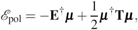(19)

where the first term represents the interactions between the dipoles and the inducing field and the second one the interactions between dipoles expressed through the polarization matrix T that will be introduced below. The minimizer μ of equation (19) is the total vector of the induced dipole moments we introduced above; it satisfies the optimality condition:

$$T\mu =\mathbf{E}.$$ (20)

3.1.1 Permanent Fields

One can apply the Ewald summation to the electric fields ${\overrightarrow{E}}_i$ for i = 1,…,N, in a similar fashion to what was described in the last section:

$${\overrightarrow{E}}_i={\overrightarrow{E}}_{i,\text{dir}}+{\overrightarrow{E}}_{i,\text{rec}}+{\overrightarrow{E}}_{i,\text{corr}}+{\overrightarrow{E}}_{i,\text{self}},$$ (21)

where

$${\overrightarrow{E}}_{i,\text{dir}}=\sum _{\overrightarrow{n}\in {\mathbb{Z}}^3}{\sum _{1\le j\le N}}^{\left(n\right)}-\frac{\partial }{\partial {\overrightarrow{r}}_i}{L}_j\left(\frac{\text{erfc}(\beta \mid {\overrightarrow{r}}_j-{\overrightarrow{r}}_i+\overrightarrow{n}\mid )}{\mid {\overrightarrow{r}}_j-{\overrightarrow{r}}_i+\overrightarrow{n}\mid }\right),$$ (22)

$${\overrightarrow{E}}_{i,\text{rec}}=\frac{1}{\pi V}\sum _{\begin{array}{c}\hfill \overrightarrow{m}\in {\mathbb{Z}}^3\hfill \\ \hfill \overrightarrow{m}\ne \overrightarrow{0}\hfill \end{array}}-\frac{\partial }{\partial {\overrightarrow{r}}_i}\left(\frac{\text{exp}(-{\pi }^2{\overrightarrow{m}}^2∕{\beta }^2)}{{\overrightarrow{m}}^2}S\left(\overrightarrow{m}\right)\text{exp}(-2i\pi \overrightarrow{m}\cdot {\overrightarrow{r}}_i)\right),$$ (23)

$${\overrightarrow{E}}_{i,\text{corr}}=\sum _{j\in M\left(i\right)}-(s_{ij}-1)\frac{\partial }{\partial {\overrightarrow{r}}_i}{L}_j\left(\frac{1}{\mid {\overrightarrow{r}}_j-{\overrightarrow{r}}_i+\overrightarrow{n}\mid }\right),$$ (24)

$${\overrightarrow{E}}_{i,\text{self}}=\frac{4{\beta }^3}{3\sqrt{\pi }}{\overrightarrow{\mu }}_{pi}.$$ (25)

The field ${\overrightarrow{E}}_{i,\text{self}}$ is a bias arising from the Ewald summation. Applying the spme method, one can approximate ${\overrightarrow{E}}_{i,\text{rec}}$ by

$${\overrightarrow{E}}_{i,\text{rec}}\approx \sum _{\overrightarrow{n}\in {\mathbb{Z}}^3}-\frac{\partial }{\partial {\overrightarrow{r}}_i}\left({\theta }_p\right(u_{1i}-n_1\left){\theta }_p\right(u_{2i}-n_2\left){\theta }_p\right(u_{3i}-n_3\left)\right)(G^R\ast Q^R)\left(\overrightarrow{n}\right)$$ (26)

as explained in section 2.

3.1.2 The Polarization Matrix

One can also apply the Ewald summation to the electric fields at site i generated by the other induced dipoles and their images, and by the images of ${\overrightarrow{\mu }}_i$, which leads to the expression of the off-diagonal term of the polarization matrix:

$$T_{ij}=T_{ij,\text{dir}}+T_{ij,\text{rec}}+T_{ij,\text{corr}}.$$ (27)

The expressions of the three terms of the right-hand side of Equation (27) are:

$$T_{ij,\text{dir}}^{\alpha \beta }={\sum _{\overrightarrow{n}\in {\mathbb{Z}}^3}}^{\left(n\right)}\frac{\partial }{\partial r_i^{\alpha }}\frac{\partial }{\partial r_j^{\beta }}\frac{\text{erfc}(\beta \mid {\overrightarrow{r}}_j-{\overrightarrow{r}}_i+\overrightarrow{n}\mid )}{\mid {\overrightarrow{r}}_j-{\overrightarrow{r}}_i+\overrightarrow{n}\mid },$$ (28)

$$T_{ij,\text{rec}}^{\alpha \beta }=\frac{2i}{V}\underset{\overrightarrow{m}\ne \overrightarrow{0}}{\sum _{\overrightarrow{m}\in {\mathbb{Z}}^3}}\frac{2i\pi \exp (-{\pi }^2{\overrightarrow{m}}^2∕{\beta }^2)}{{\overrightarrow{m}}^2}{m}^{\alpha }{m}^{\beta }\exp \left(2i\pi \overrightarrow{m}\right({\overrightarrow{r}}_j-{\overrightarrow{r}}_i\left)\right),$$ (29)

$$T_{ij,\text{corr}}^{\alpha \beta }=\sum _{j\in M\left(i\right)}(s_{ij}-1)\frac{\partial }{\partial r_i^{\alpha }}\frac{\partial }{\partial r_j^{\beta }}\left(\frac{1}{\mid {\overrightarrow{r}}_j-{\overrightarrow{r}}_i+\overrightarrow{n}\mid }\right).$$ (30)

Applying the spme method we have then:

$$T_{ij,\mathit{rec}}^{\alpha \beta }\approx \sum _{\overrightarrow{n}\in {\mathbb{Z}}^3}\frac{\partial }{\partial r_i^{\alpha }}\left({\theta }_p(u_{1i}-n_1){\theta }_p(u_{2i}-n_2){\theta }_p(u_{3i}-n_3)\right)(G^R\ast Q_j^{R\beta })\left(\overrightarrow{n}\right)$$ (31)

where $Q_j^{R\beta }$ is the multipolar array associated with the β component of the j-th induced dipole:

$$Q_j^{R\beta }(k_1,k_2,k_3)=\sum _{\overrightarrow{n}\in {\mathbb{Z}}^3}\frac{\partial }{\partial r_j^{\beta }}\left({\theta }_p(u_{1j}-k_1-K_1{n}_1){\theta }_p(u_{2j}-k_2-K_2{n}_2){\theta }_p(u_{3j}-k_3-K_3{n}_3)\right).$$ (32)

From the Ewald summation, the self-fields $T_{i,\text{self}}{\overrightarrow{\mu }}_i$, where

$$T_{i,\text{self}}^{\alpha \beta }=-\frac{4{\beta }^3}{3\sqrt{\pi }}{\delta }_{\alpha \beta },$$ (33)

also have to be included to the expression of the polarization energy that reads:

(34)

where the polarizabilities ${\alpha }_i\in {\mathbb{R}}^{3x3}$ describe the linear response to an electric field of the contribution of atom i to the density of charge. Recall that the first term represents the interactions between the inducing field and the dipoles, and the others the interactions between dipoles.

Finally, the 3N × 3N polarization matrix T, takes the form:

$$\mathrm{T}=\left(\begin{array}{ccccc}\hfill {\alpha }_1^{-1}+T_{1,\text{self}}\hfill & \hfill T_{12}\hfill & \hfill T_{13}\hfill & \hfill \cdots \hfill & \hfill T_{1N}\hfill \\ \hfill T_{21}\hfill & \hfill {\alpha }_2^{-1}+T_{2,\text{self}}\hfill & \hfill T_{23}\hfill & \hfill \cdots \hfill & \hfill T_{2N}\hfill \\ \hfill T_{31}\hfill & \hfill T_{32}\hfill & \hfill \ddots \hfill & \hfill \hfill & \hfill \hfill \\ \hfill ⋮\hfill & \hfill ⋮\hfill & \hfill \hfill & \hfill \hfill & \hfill ⋮\hfill \\ \hfill T_{N1}\hfill & \hfill T_{N2}\hfill & \hfill \hfill & \hfill \cdots \hfill & \hfill {\alpha }_N^{-1}+T_{N,\text{self}}\hfill \end{array}\right).$$ (35)

3.2 Forces

The forces associated with the polarization energy are obtained by differentiating the latter with respect to the positions of the atoms. At this point, we should remind the reader that not only does depends on the atomic positions but so does the minimizer μ. We thus obtain:

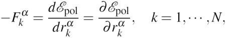where we have exploited the variational formulation of the polarization energy. More precisely, we can develop:

$$\begin{array}{cc}\hfill -F_k^{\alpha }& =-{\mu }^{†}\frac{\partial \mathbf{E}}{\partial r_k^{\alpha }}+\frac{1}{2}{\mu }^{†}\frac{\partial \mathbf{T}}{\partial r_k^{\alpha }}\mu \hfill \\ \hfill & =-\sum _{i=1}^N\frac{\partial E_i^{\beta }}{\partial r_k^{\alpha }}{\mu }_i^{\beta }+\frac{1}{2}\sum _{i=1}^N\frac{\partial {\left({\alpha }_i^{-1}\right)}^{\beta \gamma }}{\partial r_k^{\alpha }}{\mu }_i^{\beta }{\mu }_i^{\gamma }+\frac{1}{2}\sum _{i=1}^N\sum _{j\ne i}\frac{\partial T_{ij}^{\beta \gamma }}{\partial r_k^{\alpha }}{\mu }_i^{\beta }{\mu }_i^{\gamma }.\hfill \end{array}$$ (36)

The second term of the right hand side of equation (36) originates from the fact that the polarizability tensor needs to be first defined in some molecular frame and then rotated in the lab frame; similar contributions are also present in the first term due to the static dipoles and quadrupoles. Such contributions to the forces require to take the derivatives of the rotation matrices used to switch from the local frame, where the polarizabilities and multipoles are expressed, to the global frame into account. A complete derivation of these terms, which is straightforward, but very cumbersome, can be found in Ref. 34.

3.3 Iterative Schemes to Solve the Polarization Equations

In section 3.1 we introduced the polarization equations (20) which require to invert the 3N × 3N polarization matrix T to compute the induced dipoles. As N can be very large it is usually not possible to use exact methods such as LU or Cholesky factorizations whose computational cost scales as N³ (for a N × N matrix) and which require quadratic storage. A more convenient strategy is to use an iterative method. In a recent paper³⁴ we explored various iterative strategies to solve the polarization equations. We suggested that two methods seem to be especially suitable for the computation of the induced dipoles within a parallel implementation: the Preconditioned Conjugate Gradient (PCG) method and the Jacobi method coupled with Direct Inversions in the Iterative Subspace (DIIS).

We observed that the spectrum of the Polarization Matrix with Periodic Boundary Conditions computed with spme has in general almost the same structure as for nonperiodic boundary conditions, both methods have the same rate of convergence for our particular problem as what was described in our previous paper. The convergence of such methods is shown in figure 2 in comparison with the Jacobi Over-Relaxation method (JOR) which has traditionally been used in conjunction with the amoeba force field. Similarly to what was observed in direct space computation, both the JI/DIIS and PCG exhibit good convergence properties. Notice that the simple Jacobi iterations are not convergent. Although the rate of convergence is the same as for the previously studied direct space case, the decomposition of the polarization matrix T in three matrices (four with the diagonal) with particular properties makes the parallel implementation of the solvers different.

Figure 2.

Parallel scaling of the induced dipoles calculation (PCG and JI/DIIS) for the S1 system, using a separate group of processes to compute the reciprocal space contribution

4 Parallel Implementation

Let us recall the steps of both the PCG and JI/DIIS iterative methods in order to comment their parallel implementations with MPI.

Starting from an initial guess μ₀, they define a new set of induced dipoles at each iteration. In the case of the JI/DIIS solver, the new induced dipoles are obtained after one block-type Jacobi iteration followed by a DIIS extrapolation. This extrapolation requires one to assemble the so called DIIS matrix which is done by making scalar products of the past increments with the newest one.⁵⁰

Let ε be the convergence threshold and maxit the maximum number of iterations. Also, let O be the off-diagonal part of the polarization matrix T and α be the (3N × 3N) block-diagonal matrix with the polarizability tensors of the atoms of the system on its diagonal. Furthermore, let T_{sel f} be the (3N × 3N) block-diagonal matrix collecting the self terms, and D the (3N × 3N) block-diagonal part of T given by: D = α⁻¹ + T_{sel f} so that T = O+D. Then JI/DIIS can be summarized as follows:

• while it ≤ maxit and inc ≥ ε do

•  ${\tilde{\mu }}_{it+1}={\mathbf{D}}^{-1}(\mathbf{E}-{O\mu }_{it})$: Jacobi step

•  $inc={\Vert {\tilde{\mu }}_{it+1}-{\tilde{\mu }}_{it}\Vert }_{l^2\left({\mathbb{R}}^{3N}\right)}$

•  ${\mu }_{it+1}\leftarrow {\tilde{\mu }}_{it+1}$: DIIS extrapolation

• end while

The procedure is slightly more complicated for the conjugate gradient method because the new set of induced dipoles are obtained by updating them using a descent direction.

Let p_it be such a descent direction at iteration it, r_it the residual at the same iteration and p₀ = −r₀.

Then, conjugate gradient is described by the following pseudo code (preconditioned conjugate gradient only differs by the fact that T is replaced by D⁻¹T and E by D⁻¹E):

• while $it\le maxit\text{and}\Vert {\mathbf{r}}_{it}\Vert {}_{l^2\left({\mathbb{R}}^{3N}\right)}\ge ∊\mathrm{do}$

•  ${\gamma }_{it}=\frac{{\mathbf{r}}_{it}^T{\mathbf{r}}_{it}}{{\mathbf{p}}_{it}^T{\mathbf{Tp}}_{it}}$

•  μ_it+1 = μ_it +γ_itp_it : the new dipoles along the descent direction p_it

•  r_it+1 = r_it +γ_itTp_it : the updated residual

•  ${\beta }_{it+1}=\frac{{\mathbf{r}}_{it+1}^T{\mathbf{r}}_{it+1}}{{\mathbf{r}}_{it}^T{\mathbf{r}}_{it}}$

•  p_it+1 = −r_it+1+β_it+1p_it : new descent direction

• end while

In both cases, matrix-vector products are required at each iteration, these involve the current values of the dipoles for the JI/DIIS and the descent direction for the Conjugate Gradient.

In terms of a parallel implementation, the parts that require communication between processes are these matrix-vector products (communication of the dipoles or of the descent direction) and the scalar products (reductions).

A comparison between the two solvers reveals that, because of the global reductions needed to compute the DIIS matrix at each iteration, the JI/DIIS might in principle be less suited for parallelization than the PCG. There are two intertwined considerations that need to be stated. First, our implementation is based on non-blocking communication, both for the dipoles/descent directions and for the global reductions. This means that the MPI communication calls return immediately even if the processes involved are not complete: communication is performed while the computation is still going. Notice that a “MPI_Wait” or “MPI_Probe” has to be executed after the computation in order to make sure that all the processes received the needed information. The use of non-blocking communication allows one to efficiently cover the communication time, limiting thus the impact of assembling the DIIS matrix on the performances of the JI/DIIS. Second, as the communication is done before the convergence check, the converged dipoles/descent directions are always broadcast. As one needs to compute the forces in MD simulation, which require the converged dipoles to be assembled, one needs a further communication step in the PCG solver, i.e., the dipoles at convergence, whereas this is not necessary for the JI/DIIS, as the converged dipoles are already communicated. These two considerations combined explain the slightly superior performance of the JI/DIIS solver.

Note that we have improved our last parallel implementation of the solvers (that was coupled with direct space computations only) so that the only important difference between them is an additional round of communications (of the converged induced dipoles) in the case of the PCG. For this reason, we expect them to have a similar parallel behaviour.

4.1 Direct Part (real space)

In this section, we first recall the main steps of the previously studied parallel implementation of the polarization solvers without periodic boundary conditions and then explain the differences with respect to the case of the direct part of the interactions when spme is used.

When no periodic boundary conditions are imposed, as studied in Ref. 34, no cutoff is used so that global communications of the current dipoles (JI/DIIS) or descent direction (PCG) are mandatory and a particle decomposition, where the atoms are distributed among processes without taking into account their positions, suitable. These global communications, whose number grows quadratically with the number of processes, are then the obvious bottleneck to the effectiveness of the parallel implementation.

Things are more complicated for spme computations. First, the use of a cutoff for the short range real space part of the interactions makes the broadcast of all the dipoles at each iteration unnecessary: at each iteration each process only has to receive the values of the induced dipoles that are at a distance inferior to the real space cutoff.

To take advantage of this, we choose to use a spatial decomposition load balancing where each process is assigned to a region of the elementary cell. This implies that each process computes the induced dipoles arising on every atomic site lying in its part of the elementary cell. For now our algorithm only considers a spatial decomposition into slabs using a 1D-decomposition of one of the three directions and an iterative procedure has been implemented in order to adapt the size of these domains in the case of non homogeneous systems. More advanced load balancing procedures have been proposed in the literature (Ref. 51). Further developments and the tuning of these techniques for the polarization problem is under active investigation in our team and they will be included in future implementations.

To reduce the total number of messages, a good strategy is to send the induced dipoles by block: a process receives the whole part of the induced dipoles vector treated by another process as long as it needs to receive at least one of its values.

Also, we have observed that using Newton's third law, that is to compute the distance involving a pair of atom sites only once, is an important obstacle to a scalable implementation. Indeed, although it allows one to reduce the computations of such distances by half, one has to make additional communication between the processes when using this technique, which has a great impact on the parallel efficiency of the algorithm for large systems and/or when a large number of cores is employed. Furthermore, we observed that the loss in efficiency for a few cores is quickly compensated by the gain in parallel efficiency when a larger number of cores is used.

4.2 Reciprocal Space Part

The computation of the reciprocal polarization matrix/induced dipoles matrix vector product can be divided in four steps as explained in section 2.

1. The first one is to fill the multipolar array Q^R: this can be easily distributed among the processes.

2. The second one is to compute the fft of this array. We use the parallel version of the FFTW library⁵² to perform this task. As all the other parallel fft libraries, the large number of communications that it requires limits its parallel scaling to a relatively low number of cores for the 3D grids normally used for the PME method (up to 128×128×128 for example). The impact of this can be limited by increasing the real space cutoff while decreasing the size of the fft grid in order to keep the same accuracy for the PME while limiting the proportional time spent doing FFTS.

   Furthermore, as a 1D decomposition is used again to split the work among the processors (but this time the reciprocal space is divided into slabs), no performance gain can be obtained by using slabs smaller than one.

   Note also that the amoeba force field⁵³ requires one to compute two sets of induced dipoles, that correspond to two sets of electric fields created by the permanent multipoles on the atom sites with different scaling parameters.³⁷ However, the arrays involved in the fft being all real, it is possible to get all the results by calling only one complex to complex fft calculation.

   As mentioned above, the grid points are distributed among the processes with a 1D decomposition when using the MPI version of the FFTW library. Suppose that K₁, K₂ and K₃ are the sizes of the grid axis on the three dimensions the fft has to be done on. Then each MPI process treats slabs of data of size K₁ × K₂ × K_3loc, where the variation of the values of K_3loc is as small as possible between processes in order for the computational load to be well distributed. We require each process to compute the contribution to the grid of the dipoles whose scaled fractional coordinate u_3i belongs to the portion of the grid treated by this process. Depending on how the spatial decomposition is made initially, this may require a few communications between neighboring processes.

   As the B-splines are non zero only on a small portion of the grid around the scaled fractional coordinates (u_αi) of the corresponding atoms, only processes treating a neighboring portion of the grid may have contributions to the array representing the dipoles that overlap each other grids domain. In terms of communication, this means that before calling the fft routine, each process needs to receive the contributions of its neighboring processes to its part of the grid, and send its contribution to the part of the grid of its neighboring processes. Thus, these local communications are not a limiting factor in terms of parallel scaling.

3. Then the convolution in Fourier space is easily distributed among the processes and the backward fft can be directly computed in parallel as each process has already its whole portion of the grid.

4. Finally, for the same reasons as above, processes have to communicate their part of the grid to neighboring processes in order to extract the reciprocal potentials by multiplying the grid values with the appropriate B-spline values.

As explained above, reductions have to be done during the iterative procedure. This can be done without affecting the parallel scaling by using the non blocking collective operations from the MPI3 standard that allow one to cover efficiently communications with computations.

4.3 Forces

Things are less complicated for the computation of the forces associated with the polarization energy: no iterative procedure is necessary and one can make use of previous computations in order to limit the number of calls to the fft routines. Indeed, as the first step of the computation of the induced dipoles is to compute the electric fields due to the permanent multipoles of the system E, the associated multipolar grid G^R ★ Q^R($\overrightarrow{n}$) can be stored and reused to get the derivatives of the reciprocal part of this electric fields by just multiplying this grid by the appropriate derivative of the B-splines at the appropriate grid points. This cannot be done to get the electric fields created by the induced dipoles as the only associated grid that could be stored would be the one associated with the dipoles one iteration before convergence. Thus, it needs to be computed.

5 Numerical results

5.1 Computational Details

The new solvers were included in our Tinker-HP code that is a stand alone module based on elements of Tinker 6.3 and 7.0 that includes new developments introduced by our lab. The parallel implementation was tested on the Stampede supercomputer of the TACC (Texas Advanced Computing Center) whose architecture consists, for the part we did our tests on, in 6400 nodes with two intel Xeon E5-2680 CPUs with eight cores at 2.7Ghz and 32 GB of DDR3 DIMM RAM. These nodes communicate within a 56 GB/s InfiniBand network. The following numerical results are all based on computations made on this supercomputer. To benchmark our algorithms, we considered three water molecule clusters of different sizes: one of 20,000 molecules (60,000 atoms), one of 32,000 molecules (96,000 atoms) and one of 96,000 molecules (288,000 atoms). In all three cases, the convergence threshold was set to 10⁻⁵ for the dipoles increment which guarantees for energy conservation during a MD;³⁴ we used B-splines of degree 5 and a real space cutoff parameter of 1nm. The AMOEBA09 force field was used for every computation. The characteristics of these test systems, together with the PME grid sizes used and the size of the elementary cubic cell, are given in table 1. In view of using many processors, notice that the PME parameters are chosen in order to increase the computational cost of the direct part of the interactions (with better parallel scaling) and decreasing the importance of the reciprocal part, while keeping a good accuracy of the global results. From our tests, we observed that with these parameters, the computation of the polarization energy and of the associated forces represents more than 70% of a full force field single point calculation. We tested our implementation of both solvers and of the forces on the Stampede cluster and verified that we obtained the same results as the public version of TINKER up to the machine precision when the convergence criterion was pushed down to extremely small values. A first implementation showed that the poor parallel scaling of the 3D fft routines limited the global parallel scaling of the algorithm: no gain could be obtained by using more than 64–128 cores. To limit and compensate the impact of the poor parallel scaling of the fft routines, a popular strategy is to take advantage of the independence of the direct and reciprocal contributions by assigning their treatment to separate group of processes,^51,54 in a heteregenous scheme. The reciprocal space part is faster than the direct space one (by a factor that depends on the parameter β used); however the latter has a better parallel scaling: it is therefore possible to use more processors for the better scaling part by balancing the distribution of cores in such a way that the reciprocal and direct space computations take the same time doing each their part of the matrix/vector products. The heterogeneous strategy allows us to increase the scalability of our code up to 512 cores.

Table 1.

Caracteristics of the test sytems used to benchmark the parallel implementation and sizes of the fft grids. Box size is the size of the edge of the cubic box, in nanometers

System	Number of atoms	Box size	Grid Size
S1	60,000	8.40	72 × 72 × 72
S2	96,000	9.85	80 × 80 × 80
S3	288,000	14.30	128 × 128 × 128

The scaling of the PCG and JI/DIIS solvers is illustrated in figures 2–4.

Figure 4.

Parallel scaling of the induced dipoles calculation (PCG and JI/DIIS) for the S3 system using a separate group of processes to compute the reciprocal space contribution

The absolute best timings for the solvers are reported in table 2. The best timings obtained with the 6.3 version of TINKER which is parallelized with OpenMP routines and uses a different implementation of the PCG solver are also reported in supporting information for comparison. Both the JI/DIIS and the PCG solvers share a similar parallel behavior; the JI/DIIS solver exhibits a small edge in terms of parallel efficiency, which is explained in section 4, due to the additional communications happening after convergence in order to compute the forces. Nevertheless, the absolute best timings of the two solvers are comparable.

Table 2.

Absolute timings (in seconds) and number of cores used (in parentheses) for the PCG and JI/DIIS parallel solvers in our implementation (TINKER HP).

System	PCG	JI/DIIS
S1	0.45 (128)	0.44 (128)
S2	0.50 (192)	0.47 (192)
S3	0.92 (512)	0.88 (512)

The parallel computation of the forces associated with the polarization energy also naturally benefits from the separate calculation of the direct and reciprocal contributions. The scaling of our implementation is reported in figure 5. The absolute best timings are also reported in table 3, and a comparison with the best timings obtained with the 6.3 version of TINKER can be found in supporting information.

Figure 5.

Parallel scaling of the computation of the forces associated to the polarization energy for the S1, S2 and S3 systems using a separate group of processes to compute the reciprocal space contribution. Notice that negligible performance gains were observed for S1 and S2 when increasing the number of threads beyond 256.

Table 3.

Absolute best timings (in seconds) and number of cores used (in parentheses) for the computation of the forces associated to the amoeba polarization energy in our (TINKER HP) implementation

System	TINKER HP
S1	0.07 (256)
S2	0.10 (256)
S3	0.20 (512)

5.2 Further performance improvements

All the loops involved in the solvers and in the computation of the forces can be parallelized with OpenMP within each MPI process in order to limit the number of necessary communications for a given number of cores and to take advantage of the shared memory architecture within each node of the supercomputer. Furthermore, the FFTW library also enables to use such a computational paradigm. We found experimentally that the best results using this hybrid OpenMP/MPI paradigm were obtained by using 2 OpenMP threads per MPI process, allowing to improve the overall best timing of the solvers and of the computation of the forces. Notice that this hybrid paradigm can be used to extend the range of scalability of the MPI implementation; however, whenever the MPI implementation has not reached its scaling plateau, the pure MPI code is always more efficient than the hybrid one. Nevertheless, the hybrid implementation allows one to take advantage of a larger number of processors, when available.

The best overall timings obtained with the hybrid implementation are given in table 4 for both solvers and for the forces. The total best timings (energy + forces) are also reported. The numbers in the last column of table 4 give a measure of the overall computational overhead introduced by the use of polarizable force field in a PBC MD simulation: even for a system as large as S3 (almost 300,000 atoms) such an overhead can be reduced to less than a second of wall time by using the JI/DIIS solver together with the new parallel implementation. However, such numbers were computed by using a guess for the dipoles that does not take advantage of previous information, for instance, the values of the dipoles at previous steps of the simulation. As discussed in a recent publication,³⁴ the results can be further improved by using as a guess the predictor step of Kolafa's always stable predictor corrector:⁵⁵ we report in table 5 the results obtained by using such a guess, which represents our default choice for MD simulations.

Table 4.

Best Hybrid MPI/OpenMP timings (in seconds) and maximum number of CPU cores for the solvers and for the polarization forces. The overall dipoles plus forces best timings is also reported.

System	Cores	Solver		Forces	Total
		PCG	JI/DIIS
S1	256	0.32	0.30	0.04	0.34
S2	512	0.35	0.35	0.08	0.43
S3	1024	0.61	0.60	0.10	0.70

Table 5.

Best Hybrid MPI/OpenMP timings (in seconds) and maximum number of CPU cores for the solvers and for the polarization forces by using the predictor step of Kolafa's always stable predictor corrector integrator as an initial guess. The overall dipoles plus forces best timings is also reported.

System	Cores	Solver		Forces	Total
		PCG	JI/DIIS
S1	256	0.16	0.15	0.04	0.19
S2	414	0.18	0.18	0.08	0.26
S3	1024	0.32	0.30	0.10	0.40

In conclusion, our new implementation allows one to treat systems as large as S3 introducing an overhead as little as 0.7s on 1024 cores, which can be further reduced to 0.4s per time step during a MD simulation by using better initial guesses, allowing polarizable MD simulations in PBC to be performed on large and very large systems.

6 Conclusion

In this paper, we presented a new implementation of the polarization energy and associated forces for the amoeba force field which is suited to perform polarizable MD simulations using periodic boundary conditions on parallel computers. To do so, we studied the coupling of the PCG and JI/DIIS iterative solvers for polarization to spme for distributed multipoles and discussed their optimal parallel implementation. We stated in the introduction that three ingredients are needed in order to achieve an efficient implementation of a polarizable force field: a fast convergent iterative solver, a fast matrix-vector multiplication technique and an efficient parallel setup. The three points have been addressed in this paper and the resulting implementation tested on large to very large systems. Let us recapitulate the main results of this work. The first two points have been adressed by extending PCG and JI/DIIS³⁴ to the context of PBC simulations with spme. Indeed, spme transforms the involved quantities avoiding the computational bottleneck and replacing it by a calculation.

Finally, the paper addresses the third point with an extended discussion of the various technical issues that affect the specific polarization problems. The two iterative solvers have been analyzed in a real-life context, i.e., the one of MD simulations, when the forces have to be computed after the linear equations have been solved. Both solvers are well suited for a parallel implementation, however, JI/DIIS seems slightly superior to PCG for very scalable implementations. Finally, the use of only a portion of the available CPUs to do the various reciprocal space computations, while employing the other processors for the more scalable direct space ones in order to compensate the non-optimal parallel scaling of the FFTs has been addressed. This non-optimal parallel behavior is the main bottleneck of our parallel implementation which is the first to address such issues in a production code for polarizable MD.

The scaling of our implementation is overall quite good up to as many as 512–1024 cores: we would like to point out that a parallel implementation of polarizable force fields is much more challenging than for additive force fields, as solving the polarization linear systems implies a large number of synchronization barriers, one per iteration, in particular, the effect of which can be only partially mitigated by covering communication with computation.

Overall, we illustrated how our new implementation is well suited to treat large and very large systems, extending thus the range of applicability of dipole-based polarizable force fields such as amoeba to very large systems: we remark that, by using 1024 cores, as little as 0.4 second per time step is needed to handle the polarization energy and forces for a system composed of as much as 288,000 atoms, when Kolafa's predictor step is used to provide a guess for the iterative solver.

There are still various open challenges and improvements that need to be addressed for polarizable MD simulations. The use of more advanced load-balancing techniques, in the spirit of what was done for example in GROMACS,^51,56 certainly deserves future investigation. The extension of the presented machinery to other, advanced force fields, such as SIBFA⁸ and GEM⁴² is another interesting development which is being actively investigated in our groups. On a different side, we have recently proposed a complementary approach, that is, the use of polarizable continuum solvation methods instead of PBC: a comparison between the two approaches, especially for difficult systems such as highly charged metal ions or biological molecules, as well as a comparison of the performances of the two approaches, is in progress. The presented methods will also be included in the FFX package.⁵⁷ We will present in an upcoming paper an improved global scaling of the amoeba force field within the massively parallel Tinker-HP package based on Tinker 7.

Figure 1.

Norm of the increment as a function of the number of iterations for Ubiquitin and different iterative methods.

Figure 3.

Parallel scaling of the induced dipoles calculation (PCG and JI/DIIS) for the S2 system using a separate group of processes to compute the reciprocal space contribution

References

- (1).Jorgensen WL. J. Chem. Theory Comput. 2007;3:1877–1877. doi: 10.1021/ct700252g. and references therein. [DOI] [PubMed] [Google Scholar]
- (2).Warshel A, Kato M, Pisliakov AV. J. Chem. Theory Comput. 2007;3:2034–2045. doi: 10.1021/ct700127w. [DOI] [PubMed] [Google Scholar]
- (3).Cieplak P, Dupradeau F-Y, Duan Y, Wang J. J. Phys. Condens. Mat. 2009;21:333102. doi: 10.1088/0953-8984/21/33/333102. [DOI] [PMC free article] [PubMed] [Google Scholar]
- (4).Lopes PE, Roux B, MacKerell J, Alexander D. Theor. Chem. Acc. 2009;124:11–28. doi: 10.1007/s00214-009-0617-x. [DOI] [PMC free article] [PubMed] [Google Scholar]
- (5).Piquemal J-P, Jordan KD. Theor. Chem. Acc. 2012;131:1–2. [Google Scholar]
- (6).Ji C, Mei Y. Acc. Chem. Res. 2014;47:2795–2803. doi: 10.1021/ar500094n. [DOI] [PubMed] [Google Scholar]
- (7).Cisneros GA, Karttunen M, Ren P, Sagui C. Chem. Rev. 2014;114:779–814. doi: 10.1021/cr300461d. [DOI] [PMC free article] [PubMed] [Google Scholar]
- (8).Gresh N, Cisneros GA, Darden TA, Piquemal J-P. J. Chem. Theory Comput. 2007;3:1960–1986. doi: 10.1021/ct700134r. [DOI] [PMC free article] [PubMed] [Google Scholar]
- (9).Freddolino PL, Harrison CB, Liu Y, Schulten K. Nature Physics. 2010;6:751–758. doi: 10.1038/nphys1713. [DOI] [PMC free article] [PubMed] [Google Scholar]
- (10).Tong Y, Mei Y, Li YL, Ji CG, Zhang JZH. J. Am. Chem. Soc. 2010;132:5137–5142. doi: 10.1021/ja909575j. [DOI] [PubMed] [Google Scholar]
- (11).Luo Y, Jiang W, Yu H, MacKerell AD, Roux B. Faraday Discuss. 2013;160:135–149. doi: 10.1039/c2fd20068f. [DOI] [PMC free article] [PubMed] [Google Scholar]
- (12).Huang J, Lopes PEM, Roux B, MacKerell AD. J. Phys. Chem. Lett. 2014;5:3144–3150. doi: 10.1021/jz501315h. [DOI] [PMC free article] [PubMed] [Google Scholar]
- (13).Nielsen CB, Christiansen O, Mikkelsen KV, Kongsted J. J. Chem. Phys. 2007;126:154112. doi: 10.1063/1.2711182. [DOI] [PubMed] [Google Scholar]
- (14).Kongsted J, Osted A, Mikkelsen KV, Christiansen O. J. Chem. Phys. 2003;118:1620–1633. [Google Scholar]
- (15).Steindal AH, Olsen JMH, Ruud K, Frediani L, Kongsted J. Phys. Chem. Chem. Phys. 2012;14:5440–5451. doi: 10.1039/c2cp23537d. [DOI] [PubMed] [Google Scholar]
- (16).Marini A, Muñoz-Losa A, Biancardi A, Mennucci B. J. Phys. Chem. B. 2010;114:17128–17135. doi: 10.1021/jp1097487. [DOI] [PubMed] [Google Scholar]
- (17).Jacobson LD, Herbert JM. J. Chem. Phys. 2010;133:154506. doi: 10.1063/1.3490479. [DOI] [PubMed] [Google Scholar]
- (18).Arora P, Slipchenko LV, Webb SP, DeFusco A, Gordon MS. J. Phys. Chem. A. 2010;114:6742–6750. doi: 10.1021/jp101780r. [DOI] [PubMed] [Google Scholar]
- (19).Caprasecca S, Curutchet C, Mennucci B. J. Chem. Theory Comput. 2012;8:4462–4473. doi: 10.1021/ct300620w. [DOI] [PubMed] [Google Scholar]
- (20).Lipparini F, Barone V. J. Chem. Theory Comput. 2011;7:3711–3724. doi: 10.1021/ct200376z. [DOI] [PubMed] [Google Scholar]
- (21).Lipparini F, Cappelli C, Barone V. J. Chem. Theory Comput. 2012;8:4153–4165. doi: 10.1021/ct3005062. [DOI] [PubMed] [Google Scholar]
- (22).Lipparini F, Cappelli C, Barone V. J. Chem. Phys. 2013;138:234108. doi: 10.1063/1.4811113. [DOI] [PMC free article] [PubMed] [Google Scholar]
- (23).Boulanger E, Thiel W. J. Chem. Theory Comput. 2012;8:4527–4538. doi: 10.1021/ct300722e. [DOI] [PubMed] [Google Scholar]
- (24).Rick SW, Stuart SJ, Berne BJ. J. Chem. Phys. 1994;101:6141–6156. [Google Scholar]
- (25).Verstraelen T, Speybroeck VV, Waroquier M. J. Chem. Phys. 2009;131:044127. doi: 10.1063/1.3187034. [DOI] [PubMed] [Google Scholar]
- (26).Piquemal J-P, Chelli R, Procacci P, Gresh N. J. Phys. Chem. A. 2007;111:8170–8176. doi: 10.1021/jp072687g. [DOI] [PubMed] [Google Scholar]
- (27).Lamoureux G, Roux B. J. Chem. Phys. 2003;119:3025–3039. [Google Scholar]
- (28).Mills MJ, Popelier PL. Comp. Theor. Chem. 2011;975:42–51. [Google Scholar]
- (29).Applequist J, Carl JR, Fung K-K. J. Am. Chem. Soc. 1972;94:2952–2960. [Google Scholar]
- (30).Thole B. Chem. Phys. 1981;59:341–350. [Google Scholar]
- (31).Wang J, Cieplak P, Li J, Wang J, Cai Q, Hsieh M, Lei H, Luo R, Duan Y. J. Phys. Chem. B. 2011;115:3100–3111. doi: 10.1021/jp1121382. [DOI] [PMC free article] [PubMed] [Google Scholar]
- (32).Ponder JW, Wu C, Ren P, Pande VS, Chodera JD, Schnieders MJ, Haque I, Mobley DL, Lambrecht DS, DiStasio RA, Head-Gordon M, Clark GNI, Johnson ME, Head-Gordon T. J. Phys. Chem. B. 2010;114:2549–2564. doi: 10.1021/jp910674d. [DOI] [PMC free article] [PubMed] [Google Scholar]
- (33).Gordon MS, Slipchenko L, Li H, Jensen JH. Annu. Rep. Comput. Chem. 2007;3:177–193. [Google Scholar]
- (34).Lipparini F, Lagardère L, Stamm B, Cancès E, Schnieders M, Ren P, Maday Y, Piquemal J-P. J. Chem. Theory Comput. 2014;10:1638–1651. doi: 10.1021/ct401096t. [DOI] [PMC free article] [PubMed] [Google Scholar]
- (35).Wang W, Skeel RD. J. Chem. Phys. 2005;123:164107. doi: 10.1063/1.2056544. [DOI] [PubMed] [Google Scholar]
- (36).Sagui C, Pedersen LG, Darden TA. J. Chem. Phys. 2004;120:73–87. doi: 10.1063/1.1630791. [DOI] [PubMed] [Google Scholar]
- (37).Lipparini F, Lagardère L, Raynaud C, Stamm B, Cancès E, Mennucci B, Schnieders M, Ren P, Maday Y, Piquemal J-P. J. Chem. Theory Comput. 2015;11:623–634. doi: 10.1021/ct500998q. [DOI] [PMC free article] [PubMed] [Google Scholar]
- (38).Caprasecca S, Jurinovich S, Lagardère L, Stamm B, Lipparini F. J. Chem. Theory Comput. 2015;11:694–704. doi: 10.1021/ct501087m. [DOI] [PubMed] [Google Scholar]
- (39).Ewald PP. Ann. Phys. 1921;369:253. [Google Scholar]
- (40).Darden T, York D, Pedersen L. J. Chem. Phys. 1993;98:10089–10092. [Google Scholar]
- (41).Essmann U, Perera L, Berkowitz ML, Darden T, Lee H, Pedersen LG. J. Chem. Phys. 1995;103:8577–8593. [Google Scholar]
- (42).Cisneros GA, Piquemal J-P, Darden TA. J. Chem. Phys. 2006;125:184101. doi: 10.1063/1.2363374. [DOI] [PMC free article] [PubMed] [Google Scholar]
- (43).Smith ER. Proc. R. Soc. A. 1981;375:475–505. [Google Scholar]
- (44).Aguado A, Madden PA. J. Chem. Phys. 2003;119:7471–7483. [Google Scholar]
- (45).Toukmaji A, Sagui C, Board J, Darden T. J. Chem. Phys. 2000;113:10913–10927. [Google Scholar]
- (46).Nymand TM, Linse P. J. Chem. Phys. 2000;112:6152–6160. [Google Scholar]
- (47).Sala J, Guàrdia E, Masia M. J. Chem. Phys. 2010;133:234101. doi: 10.1063/1.3511713. [DOI] [PubMed] [Google Scholar]
- (48).Sagui C, Pedersen LG, Darden TA. J. Chem. Phys. 2004;120:73–87. doi: 10.1063/1.1630791. [DOI] [PubMed] [Google Scholar]
- (49).Smith W. CCP5 Newsletter. 1998;46:18–30. [Google Scholar]
- (50).Rohwedder T, Schneider R. J. Math. Chem. 2011;49:1889–1914. [Google Scholar]
- (51).Hess B, Kutzner C, Van Der Spoel D, Lindahl E. J. Chem. Theory Comput. 2008;4:435–447. doi: 10.1021/ct700301q. [DOI] [PubMed] [Google Scholar]
- (52).Frigo M, Johnson SG. FFTW: An adaptive software architecture for the FFT. 1998. [Google Scholar]
- (53).Ponder JW, Wu C, Ren P, Pande VS, Chodera JD, Schnieders MJ, Haque I, Mobley DL, Lambrecht DS, DiStasio RA, Head-Gordon M, Clark GNI, Johnson ME, Head-Gordon T. J. Phys. Chem. B. 2010;114:2549–2564. doi: 10.1021/jp910674d. [DOI] [PMC free article] [PubMed] [Google Scholar]
- (54).Phillips JC, Braun R, Wang W, Gumbart J, Tajkhorshid E, Villa E, Chipot C, Skeel RD, Kale L, Schulten K. J. Comput. Chem. 2005;26:1781–1802. doi: 10.1002/jcc.20289. [DOI] [PMC free article] [PubMed] [Google Scholar]
- (55).Kolafa J. J. Comput. Chem. 2004;25:335–342. doi: 10.1002/jcc.10385. [DOI] [PubMed] [Google Scholar]
- (56).Pronk S, Páll S, Schulz R, Larsson P, Bjelkmar P, Apostolov R, Shirts MR, Smith JC, Kasson PM, van der Spoel D, Hess B, Lindahl E. Bioinformatics. 2013;29:845–854. doi: 10.1093/bioinformatics/btt055. [DOI] [PMC free article] [PubMed] [Google Scholar]
- (57).Schnieders MJ, Fenn TD, Pande VS. J. Chem. Theory Comput. 2011;7:1141–1156. doi: 10.1021/ct100506d. [DOI] [PubMed] [Google Scholar]