Current extinction rates of reptiles and amphibians

Significance

It is hard to know how many species have gone extinct so far because it is difficult to prove that something not seen recently is really gone forever. This paper uses a new, highly conservative statistical method to infer the number of extinct amphibian and reptile species across the world. Frogs are of particular concern because an invasive fungus has recently caused many populations to collapse. The data are lists of specimens in museum collections. The method provides sensible results when the data are randomized or artificial extinctions are imposed. It suggests that about 200 frog extinctions have occurred and hundreds more will be lost over the next century, so we are on pace to create a mass extinction.

Abstract

There is broad concern that a mass extinction of amphibians and reptiles is now underway. Here I apply an extremely conservative Bayesian method to estimate the number of recent amphibian and squamate extinctions in nine important tropical and subtropical regions. The data stem from a combination of museum collection databases and published site surveys. The method computes an extinction probability for each species by considering its sighting frequency and last sighting date. It infers hardly any extinction when collection dates are randomized and it provides underestimates when artificial extinction events are imposed. The method also appears to be insensitive to trends in sampling; therefore, the counts it provides are absolute minimums. Extinctions or severe population crashes have accumulated steadily since the 1970s and 1980s, and at least 3.1% of frog species have already disappeared. Based on these data and this conservative method, the best estimate of the global grand total is roughly 200 extinctions. Consistent with previous results, frog losses are heavy in Latin America, which has been greatly affected by the pathogenic chytrid fungus Batrachochytrium dendrobatidis. Extinction rates are now four orders-of-magnitude higher than background, and at least another 6.9% of all frog species may be lost within the next century, even if there is no acceleration in the growth of environmental threats.

Obtaining concrete estimates of extinction tallies for major taxonomic groups has proven to be elusive, with the literature veering between conservative counts based on thorough assessments of well-known species to much higher figures based on global-scale considerations of threat levels (1–5). Uncertainty is so great that, for example, the 2004 Global Amphibian Assessment (1) used by the International Union for the Conservation of Nature (IUCN) hazarded that anywhere between 9 and 122 amphibians might have gone extinct since 1980. Another analysis (2) suggested a range of 28–201. Meanwhile, comprehensive reviews of threats to reptiles (5) offered no estimate of the number of extinct species and sidestepped the matter of whether it might be large.

These sorts of questions are still wide open because (i) it is difficult to distinguish species that are highly endangered and rarely sighted from species that are actually extinct, and (ii) researchers have lacked a robust statistical protocol for estimating extinction tallies (6). A means of addressing these concerns is provided by a Bayesian approach that involves computing probabilities of sightings (Materials and Methods), which like a recently published algorithm (6) yields highly accurate posterior extinction probabilities in simulations. As a result, the summed posteriors constitute reasonable estimates of the total number of species to have gone extinct in a particular area (Tables 1 and 2). The probabilities are dependent upon the exact choice of Bayesian priors and on other details of implementation, but the method is consistently conservative and it is optimal for detecting single-digit extinction percentages of the kind reported here (Materials and Methods).

Table 1.

Estimated numbers of frog extinctions in studied geographic regions

Region	Species	Prior	Posterior	Extinct	CI
Southeastern United States	66	0.0283	0.0011	0.07	0.03–0.12
Mesoamerica	384	0.1341	0.0462	17.74	13.61–22.52
Brazil	517	0.0895	0.0265	13.69	9.48–18.61
Southern Europe	32	0.0060	0.0000	0.00	–
East Africa	177	0.1259	0.0503	8.90	5.44–13.07
Madagascar	187	0.1277	0.0591	11.06	6.74–16.10
South Asia	142	0.0419	0.0101	1.43	0.24–3.07
Sunda	293	0.0193	0.0012	0.35	0.13–0.62
Sahul	412	0.1164	0.0528	21.77	15.70–28.52
Global	2,164	0.0927	0.0305	66.05	56.00–76.98

Counts consistently exceed those obtained by randomizing the data (Table S1). “Species” is number of species analyzed. “Prior” is average extinction probability based on a first-pass analysis of the data. “Posterior” is average extinction probability based on a reanalysis using the computed prior. “Extinct” is sum of extinction probabilities. “CI” is bootstrapped 95% confidence interval.

Table 2.

Estimated numbers of squamate extinctions in studied geographic regions

Region	Species	Prior	Posterior	Extinct	CI
Southeastern United States	164	0.0690	0.0163	2.67	1.06–5.06
Mesoamerica	748	0.0908	0.0197	14.74	11.09–18.95
Brazil	300	0.0494	0.0059	1.77	1.02–2.80
Southern Europe	97	0.0796	0.0192	1.86	0.69–3.83
East Africa	283	0.1083	0.0307	8.68	5.85–12.23
Madagascar	223	0.1183	0.0447	9.96	6.44–14.11
South Asia	251	0.1130	0.0380	9.55	6.46–13.22
Sunda	449	0.0419	0.0057	2.57	1.33–4.35
Sahul	906	0.0522	0.0073	6.63	4.64–9.07
Global	3266	0.0744	0.0165	53.99	45.96–62.41

Column names are as in Table 1. See also Table S2.

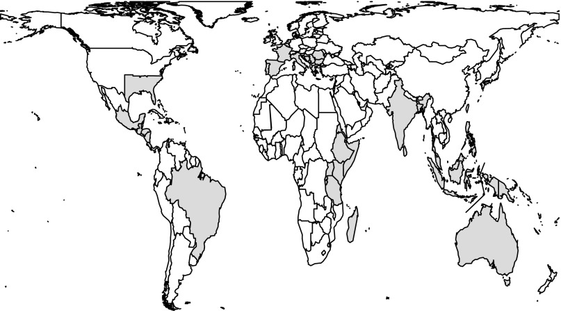
The new equation is applied here to anuran, caudatan, and squamate museum specimen records and published observations that encompass nine major geographic regions (Fig. S1). Although the dataset does not include unpublished field observations, the identifications used here constitute the only information that can be used in a study of this kind. Study regions were selected based on the amount of available data and to provide broad coverage emphasizing the tropics. These regions collectively include most of the hotspots for amphibian diversity (3) and for vertebrates in general (4), and they are large and widely dispersed enough that they are likely to be representative. The analyses used individual specimen records primarily drawn from HerpNET (www.herpnet.org) and a series of databases focusing on particular regions or museums. Additional information was drawn from 361 publications that documented recent sightings in particular localities, and public databases were used to vet and update species names. The dataset includes at least one observation each for 2,708 of 6,355 frog species recognized as valid by AmphibiaWeb (amphibiaweb.org) (42.6%) and 4,105 of 9,267 squamate species recognized by the Reptile Database (www.reptile-database.org) (44.3%).

Fig. S1.

Geographic regions included in the analysis.

Results

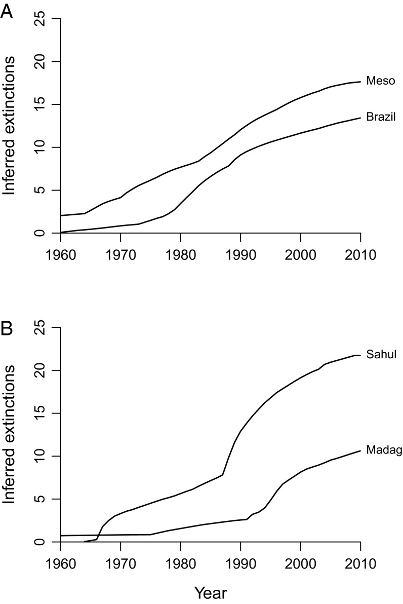
Cumulative extinction probability curves suggest that anuran extinction rates were negligible before the 1970s, and since then have been considerable and sustained (Fig. 1). There is substantial decoupling among regions and between groups (Table 1). For example, the number of extinctions in the southeastern United States and southern Europe is apparently zero, in line with previously published expectations that tropical species are more threatened (1, 4, 5), and frog extinctions usually exceed squamate losses in the same regions. Because most of the apparent squamate extinctions except those in Mesoamerica, Madagascar, and possibly South Asia seem to represent either local extirpations or other confounding factors (Supporting Information), the data only provide clear evidence of extinction pulses of frogs and only in a few specific areas: Mesoamerica, Brazil, Madagascar, and the Sahul region. Most of the apparent extinctions in Sahul pertain to New Guinea, where the dataset is of good quality (Fig. S2).

Fig. 1.

Cumulative numbers of inferred anuran extinctions in (A) Mesoamerica and Brazil and (B) Madagascar and the Sahul region (where extinctions are strongly concentrated in New Guinea). Figures are sums of individual extinction probabilities (see Table 1 for frogs and Table 2 for squamates) and are extremely conservative (Materials and Methods and Figs. 4 and 5). Global grand totals are 66.1 frog extinctions and 54.0 squamate extinctions.

Fig. S2.

Size of the dataset representing New Guinea. A square-root scale is used on the y axis to make smaller values more visible.

The figures for these regions weakly suggest an acceleration in extinction rates during the 1980s and early 1990s (Fig. 1). If real, this pattern might relate to the Batrachochytrium dendrobatidis epidemic, which has been strongly implicated in major population declines of anurans throughout Central America (7) and Australia (8) and is a potential factor in Brazil (9). B. dendrobatidis also infects plethodontid salamanders and is thought to be responsible for Central American salamander population declines (7). However, B. dendrobatidis is absent from New Guinea (10) and Madagascar (11), where the current data suggest there has been a substantial number of extinctions. The data also do not prove that there has been a truly catastrophic mass extinction in Central America, even though numerous population crashes have been observed (7). Furthermore, B. dendrobatidis has had little or no effect on populations in Europe (12), Asia (13), and mainland Africa (14) despite being present. Therefore, rates of anuran loss cannot yet be tied to B. dendrobatidis in a consistent manner.

Variation among countries is also difficult to relate to their environmental and socioeconomic differences in a broad-brush manner. For example, the possible extinction pulse in Madagascar may stem from the fact that its human population has more than doubled since 1985, at which point 66% of its rain forests had already been eliminated (15). High extinction rates in Brazil and New Guinea also might involve deforestation. However, deforestation in South Asia and the Sunda region appears to have had little or no impact.

Factors other than the B. dendrobatidis epidemic and habitat destruction might be important locally, but if the current analysis is accurate then they are less plausible as single agents of extinction on a global scale. No one has suggested that the numerous introductions of exotic reptile and amphibian species in the United States have resulted in extinctions of native species, and introductions in the tropics have been minimal. The cane toad Rhinella marina has been introduced to Australia and New Guinea, where it might be a factor, but also the Philippines, the United States, and other countries where no major losses of amphibians appear to have occurred (Table 1). Economic exploitation has been implicated by the IUCN in very few major population declines of individual amphibians and reptile species and appears to have spatially restricted effects (5, 8). Finally, this analysis is unable to directly quantify the effects of climate change, but the early onset and steady pace of extinctions in most areas (Fig. 1) is inconsistent with a recent major impact. This point will, however, become irrelevant as global warming continues to accelerate.

Discussion

In sum, there are two major patterns in the regional data. First, despite spatial heterogeneity the number of frog extinctions seems to have been much higher in relative terms than the number of squamate extinctions (Table 1 vs. Table 2). Second, a substantial extinction pulse in Latin America is most plausibly related to the B. dendrobatidis epidemic, although it might involve other factors such as deforestation or the spread of invasive species.

Total global losses for the entire study period through 2010 are 3.05% for frogs (Table 1). This figure is equivalent to ∼6,355 × 0.0305 = 194 extinctions if the true global tally is proportional to estimates for the regions studied here. Figures for caudatans are similar in relative terms (Materials and Methods). The anuran total to date is higher than previously reported values (2). Therefore, one could argue that the tallies might represent regional extirpations, taxonomic errors, and cases in which population crashes have not yet led to actual extinctions. Cases of extirpation and error appear to be rare with respect to frogs, although nuisance factors are important for squamates (Supporting Information). It is also impossible to say whether some of the inferred frog extinctions do represent steep population declines. Regardless, there are many good reasons to think the counts are conservative: (i) the analytical method is designed to infer less extinction when data are lacking or when a species is found in multiple areas; (ii) it is also unlikely to detect extinctions that have occurred within the last decade or two (Fig. 2); (iii) the results have been skewed downward by assuming that extinctions could have taken place as early as 1900, long before many species were even described; (iv) a substantial number of species may have disappeared before being documented in museum collections; (v) rare species are more often omitted from the analyses because multiple sightings are required to compute an extinction probability; (vi) some seemingly widespread species, especially in the tropics, may actually consist of cryptic species complexes that include locally rare and geographically restricted members (16); (vii) processes such as human population growth, habitat destruction, and climate change accelerated through the study interval; and (viii) many species may already be doomed to extinction because their current population sizes are unviable.

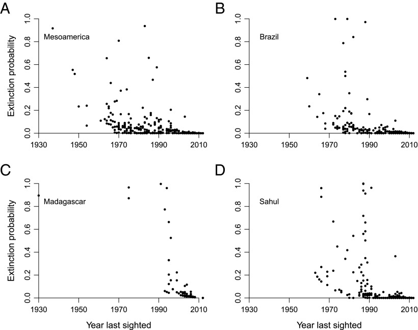
Fig. 2.

Relationship between the current extinction probability and the last year of collection for frogs from the Mesoamerica (A), Brazil (B), Madagascar (C), and the Sahul region (D).

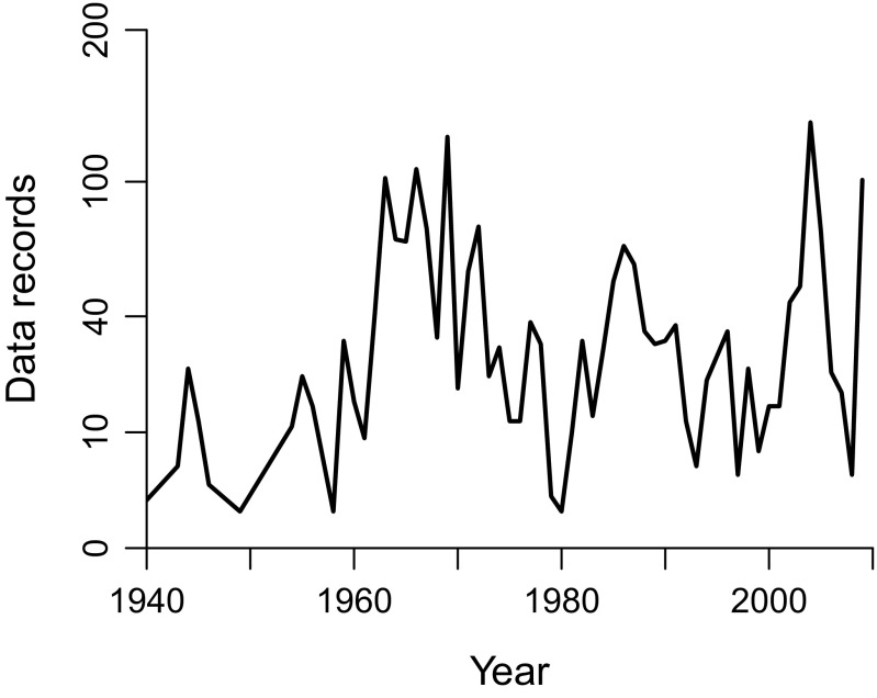
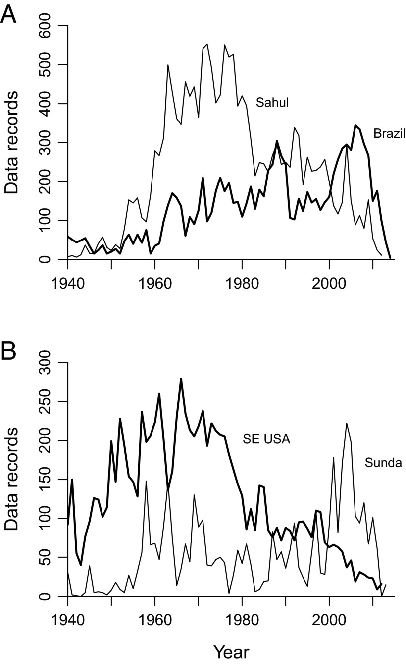
Even though the first point is straightforward, the fact that the analysis only recovers absolutely large anuran extinction pulses in selected regions (Fig. 1 and Table 1) raises the question of whether these pulses might simply reflect regional declines in sampling. This suspicion is hard to square with actual sampling trends (Fig. 3). For example, extinctions are relatively common in both Brazil and the Sahul region but the data tallies go in opposite directions (Fig. 3A). Meanwhile, little or no extinction is inferred for frogs from the southeastern United States or Sunda region, and yet the former dataset shows a decline much like that in the Sahul region, whereas the latter exhibits high variation with an overall upward trend (Fig. 3B). These patterns strengthen the argument that the figures reported in Table 1 are absolute minima.

Fig. 3.

Size of anuran datasets representing regions with high (A) and low (B) extinction estimates. (A) The Sahul region (thin line) and Brazil (thick line). (B) The Sunda region (thin line) and southeastern United States (thick line).

Because a method like the one used here infers little extinction in the absence of data, the true scope of the current mass extinction will remain unclear until there is much more intensive sampling in the tropics. Indeed, this paper is not intended to provide a definitive answer because the data include a myriad of complexities. It only offers a conservative lower bound that is an approximation of current knowledge. Despite this fact, the evidence does suggest that there has been a massive increase in the extinction rate over the long-term background average. Fossil data indicate that the background rate for reptiles and amphibians is even lower than the approximate 22% per species per million year rate for mammals (17) (Materials and Methods). A cumulative loss on the order of several percent in a few decades (Fig. 1 and Table 1) therefore implies that current rates are about four orders of magnitude higher than normal. Indeed, average extinction rates observed during 1971–2000 suggest that, about 6.9% of anuran species may be lost within the next century (Materials and Methods). This rate may seem slow on a human time scale, but it is a conservative minimum estimate and human impacts are intensifying. Thus, the data suggest that a runaway train of extinction is now likely to produce what would be seen as a global mass extinction on the ultimately more important landscape of geological time. Mitigating this crisis will require strong ongoing support of monitoring by field ecologists and museum scientists (18).

Materials and Methods

Geographic Regions.

The analyses focused on nine mostly large geographic regions with distinct biotas that were chosen to cover major hotspots of biodiversity (3) and conservation threat (4); they capture large fractions of all low-latitude biogeographic regions, including both humid and arid biomes (Fig. S1). Parts of the United States and Europe were analyzed to broaden the socioeconomic and demographic scope of areas included in the study. The focal regions were the southeastern United States (Alabama, Arkansas, Florida, Georgia, Louisiana, Mississippi, North Carolina, South Carolina, Tennessee, and Texas east of 100° W); Mesoamerica (Belize, Costa Rica, El Salvador, Guatemala, Honduras, Nicaragua, Panama, and tropical Mexico; i.e., all Mexican states centered below the Tropic of Cancer); Brazil; southern Europe (Albania, Bosnia and Herzegovina, Croatia, Cyprus, Bulgaria, France, Greece, Italy, Kosovo, Macedonia, Malta, Montenegro, Portugal, Romania, Serbia, Slovenia, and Spain); East Africa (Burundi, Djibouti, Eritrea, Ethiopia, Kenya, Rwanda, Somalia, Tanzania, and Uganda); Madagascar; low-altitude South Asia (Bangladesh, India, and Sri Lanka); the Sunda Shelf region (Brunei, Indonesia, Malaysia, the Philippines, and Singapore); and the Sahul region (New Guinea, including Papua New Guinea and the Indonesian part of the island, and Australia). Data were sparse for the remaining subtropical and tropical regions.

Data Sources.

Analyses were restricted to species listed as being valid by AmphibiaWeb (amphibiaweb.org) or the Reptile Database (www.reptile-database.org). Lists of specimens were downloaded from HerpNET (www.herpnet.org), the Online Zoological Collections of Australian Museums (OZCAM) website (ozcam.org.au), the American Museum of Natural History website (AMNH: www.amnh.org), the Field Museum of Natural History website (fm1.fieldmuseum.org/collections/search.cgi?dest=herps&action=form), and the Muséum national d’Histoire naturelle website (https://science.mnhn.fr). Additional records for East Africa were directly provided by the AMNH and the Natural History Museum in London. Data for Brazil were retrieved from the speciesLink Network (www.splink.org.br). Institutions providing large numbers of data records are listed in the Supporting Information.

Additional data were drawn from the primary literature to make sure that undersampling was not responsible for high extinction count estimates (although the Bayesian method actually tends to underestimate extinction when sampling is persistently poor). The literature search focused on papers published over the past 15 y and, respectively, yielded 53, 18, 48, 61, 95, 71, and 15 publications for the Mesoamerican, Southern European, East African, Malagasy, South Asian, Sunda Shelf, and New Guinea datasets. The United States, Brazilian, and Australian datasets were deemed adequate without augmentation.

Data Preparation.

Invalid names were corrected by referring to a list of synonyms and outdated genus-species combinations downloaded from the Integrated Taxonomic Information System website (www.itis.gov). Records of 91 extralimital species, invasive species, and species found only on small islands were removed by hand. Threat status was based on the IUCN Red List of Threatened Species (www.iucnredlist.org), with some updates drawn from the Australian Environment Protection and Biodiversity Conservation Act list (www.environment.gov.au).

Species sampled only in 1 y were omitted from the analysis. Data records were grouped by collection year and location. Sample locations were defined as states or provinces for Brazil, India, Indonesia, Malaysia, Mexico, the Philippines, and the United States, Interim Biogeographic Regionalization for Australia regions for Australia, and otherwise entire countries. For published data, locations were defined as reported by the authors.

Extinction Probability Equation.

Numerous methods of evaluating individual species have been proposed (19, 20) but they perform poorly when evaluated using either empirical data (20, 21) or simulations (22). Most of them also provide hypothesis test statistics (i.e., P values) instead of actual extinction chances, and as such are categorically unusable for the present purpose of inferring extinction counts. Posterior probabilities were instead computed using a simple Bayesian method, which performs robustly in a variety of simulations similar to those previously published (6). The probabilities it generates are strongly related to the last year of sighting (Fig. 2) but the correlation is erratic because other factors come into play.

The computation works by combining an agnostic, 0.5 prior extinction probability with joint conditionals calculated separately for the two hypotheses that a given species has survived or gone extinct. It is assumed that extinction operates on a continuous basis, so the extinction probability declines exponentially through time and is therefore lowest in the most recent year. Assuming a uniform distribution instead would make little difference to the results because the exponentially distributed per interval prior changes very slowly. Varying the overall prior of 0.5 uniformly over the range 0–1 would have no effect at all.

The conditional computations are based on a published combinatoric equation (23) that compares the number of ways a species’ sightings can be located within its observed range to the number of ways they can be located across the species’ hypothesized range. These probabilities are based on the numbers of potential sightings (i.e., those of all species found in the same geographic area) and of actual sightings. The conditional based on the survival hypothesis assumes that each species actually ranges through the whole study interval; the conditionals based on hypothesized extinction dates assume that the ranges go up to the base of the relevant intervals. The conditionals are set to zero for all extinction dates that equal or precede the last sighting. Bayes’ theorem is then applied to compute a posterior extinction probability for each interval. The summed probabilities are computed for all species and then averaged to obtain a rate for the entire dataset. Finally, this mean probability is recycled as a prior and the individual species values are recomputed. Simulations show that this last step biases the figures downward when actual probabilities are high, but when they are very low recycling produces more accurate estimates.

This method could be applied to simple presence–absence data. However, there is much additional information in the form of sighting frequencies within intervals. Therefore, the calculations are based on counts of sightings of each focal species in each interval relative to counts of all sightings in each interval (Fig. 3).

To make the analyses more realistic, the data are analyzed separately for each local geographic area (country or state/province) and the resulting posteriors are then multiplied to obtain an overall extinction probability for each species. This approach is highly conservative because poor data in any area will result in a low individual posterior and therefore a low product. For example, if a species found in three areas has posteriors of 0.5, 0.5, and 0.1, the overall extinction probability is only 0.025. In practice, the method almost never infers that a species found in multiple areas is extinct.

The computations must consider a fixed window of time. This window could equal the span between the first and last observation of the taxonomic group in a given region. However, using a fixed window across all regions seems more objective. The computation will yield higher extinction probabilities when the window is short. In principle, it would be admissible to assume that no extinctions could have taken place before about 1950 because the current analysis suggests that few or none occurred before the 1960s (Fig. 1). To make the analyses more conservative, the window is defined to run from the year 1900 to the last observation of the group in the relevant region. Imposing this rule has little effect in terms of truncating older data because there are few 19th century data records in most regions.

Confidence Intervals.

The samples of species (Tables 1 and 2) are partial relative to total global diversity, making it important to estimate uncertainty in the counts. Confidence limits are easy to compute using a bootstrap protocol in which posterior extinction probabilities are drawn with replacement from the empirical set, the values are summed, and the procedure is iterated 10,000 times. Tables 1 and 2 report the 95% confidence limits derived using this procedure.

Performance with Randomized Data.

Any method will flag some species as extinct regardless of whether any extinctions have occurred in the first place. It is therefore important to show that false-positives are rare by considering what would happen if we could be sure there was no extinction at all. This question is easily answered by randomizing combinations of collection years and spatial locations plus identifications across the entire set of data records for each region (e.g., records of all frogs from Brazil). For example, a date of 1900 might be substituted for one of 2000 in an identification of some species from some place. Records are grouped by geographic area (country or state/province) to make sure that spatial variation in sampling intensity is not altered. By definition, the randomization protocol leaves the number of data records in each year unchanged. It also has almost no visible effect on the number of species sampled in a given year (Fig. S3), which shows that inferred extinctions cannot be attributed to a trend toward only sampling nonthreatened species. The results of a single trial each for the four key frog datasets are illustrated in Fig. 4. These very low cumulative extinction probability sums (see also Tables S1 and S2) show that the trends summarized in Fig. 1 and Table 1 cannot be dismissed as an artifact of the method: if a species is not actually extinct it almost never infers a high extinction probability. Thus, the extinction tallies reported in this paper are likely to be absolute minimums, regardless of whether sampling is rich or poor.

Fig. S3.

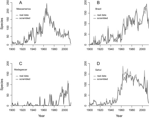
Number of species sampled per year in the actual data for frogs from (A) Brazil, (B) Mesoamerica, (C) Madagascar, and (D) the Sahul region (thin black lines) and datasets in which the years of collection have been randomized (thick gray lines; see also Fig. 4). Small offsets and the lack of consistent trends demonstrate that collectors are not focusing more strongly on particular groups of species.

Fig. 4.

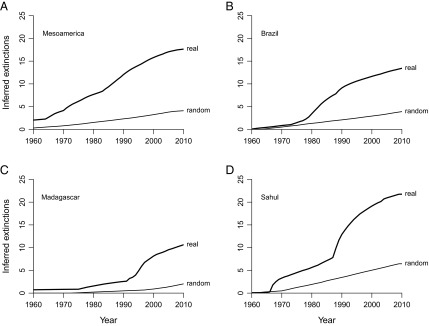
Simulated extinction proportions recovered by Bayesian analysis in the presence and absence of extinction. Data are for (A) Mesoamerica, (B) Brazil, (C) Madagascar, and (D) the Sahul region. Upper lines (“real”) show actual values. Lower lines (“random”) show data produced by randomizing collection dates, which obliterates any signal of true extinction.

Table S1.

Frog extinction probabilities computed on the basis of randomized data

Region	Prior	Posterior	Extinct
Southeastern United States	0.0351	0.0025	0.16
Mesoamerica	0.0766	0.0107	4.13
Brazil	0.0595	0.0079	4.07
Southern Europe	0.0342	0.0017	0.05
East Africa	0.0653	0.0095	1.67
Madagascar	0.0775	0.0122	2.30
South Asia	0.0418	0.0083	1.25
Sunda	0.0196	0.0010	0.27
Sahul	0.0799	0.0157	6.47
Global	0.0604	0.0083	17.85

Prior = average extinction probability based on a first-pass analysis of the data. Posterior = average extinction probability based on a reanalysis using the computed prior. Extinct = sum of extinction probabilities.

Table S2.

Squamate extinction probabilities computed on the basis of randomized data

Region	Prior	Posterior	Extinct
Southeastern United States	0.0813	0.0141	2.29
Mesoamerica	0.0768	0.0110	8.26
Brazil	0.0380	0.0030	0.89
Southern Europe	0.0775	0.0119	1.17
East Africa	0.0858	0.0162	4.67
Madagascar	0.1097	0.0372	8.48
South Asia	0.0524	0.0076	1.97
Sunda	0.0294	0.0031	1.40
Sahul	0.0451	0.0044	3.99
Global	0.0577	0.0072	23.65

Column names are as in Table S1.

Performance with Truncated Data.

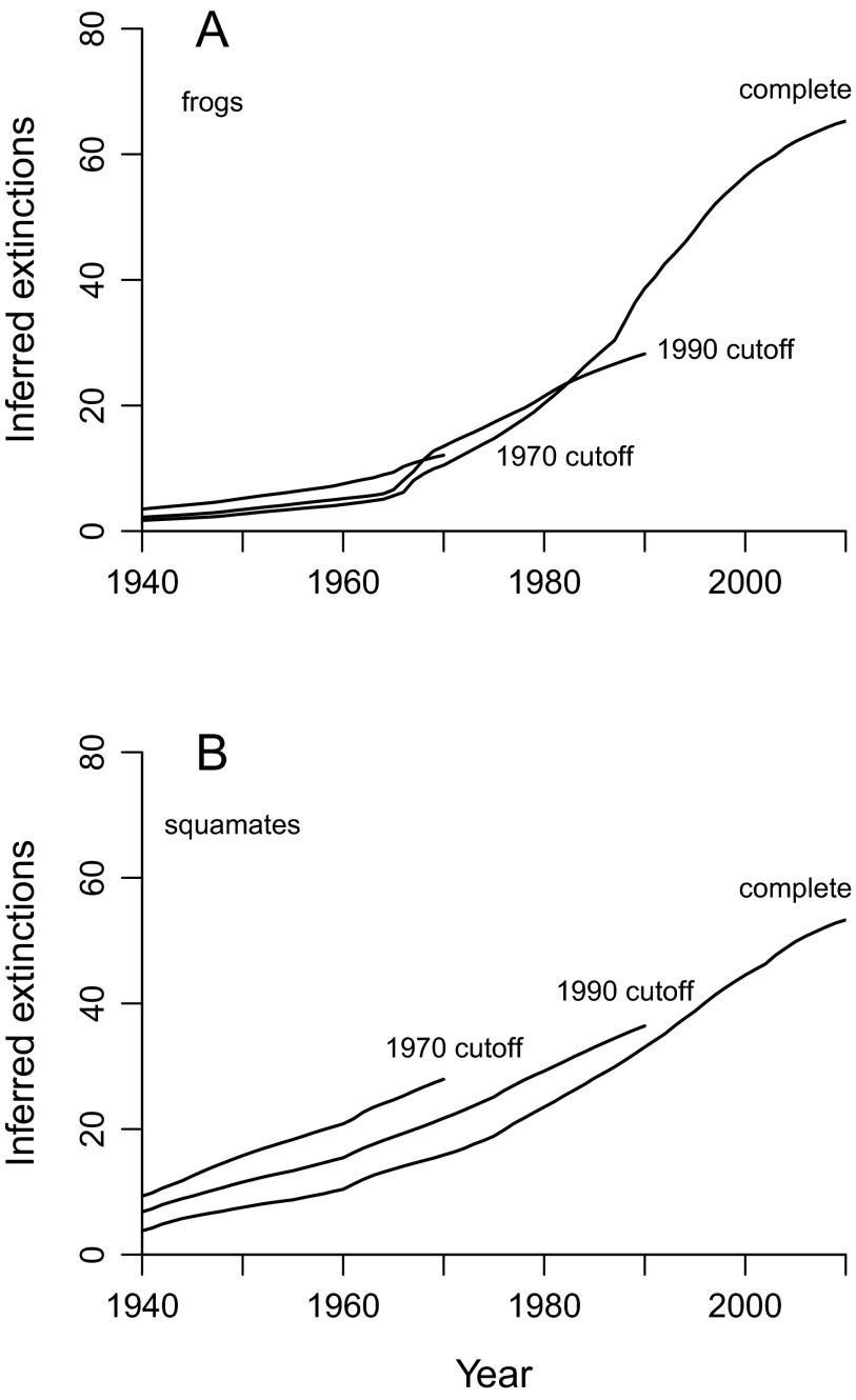
A poor method might infer many spurious extinctions because the data are truncated at the present. In other words, it might be fooled by the fact that many species have not been sighted recently simply at random, even though they will be sighted again in the future. To test for this bias, the global frog data were truncated at 1990 and then again at 1970 and the extinction probabilities were recomputed. The results suggest that censorship has virtually no effect on the running tally of inferred extinctions (Fig. S4). There are also fair correlations between the through-1970 and current probabilities (Spearman’s rank-order correlation ρ = 0.592, P < 0.001) and between through-1990 and current probabilities (ρ = 0.612, P < 0.001), which is noteworthy because the truncated probabilities are consistently low and therefore more subject to random sampling error.

Fig. S4.

(A and B) Effect of truncating the data records at either 1970 or 1990.

Performance with Simulated Extinction.

The degree of conservativeness of the method when applied to real data can also be shown in a straightforward way by means of a Monte Carlo simulation analysis. The algorithm involves randomly adding a number of extinction events to an empirical dataset and seeing whether the analytical method recovers the correct extinction proportion. (i) Extinction events are randomly produced on the basis of an assumed per year extinction probability. To reflect the fact that major extinction threats have increased through time, a zero probability is assumed for years before 1900. (ii) All actual presences of a species younger than the simulated extinction event are removed from the dataset. (iii) The number of species going extinct is divided by the total to produce a simulated proportion. (iv) Bayesian computations are applied to the data and the sum of extinction probabilities is divided by the number of analyzed species to produce an inferred proportion. (v) The analysis is repeated after varying the assumed extinction probability.

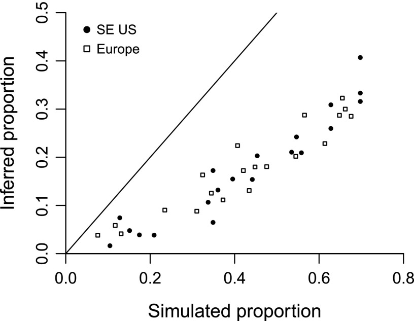
Interpreting the results would be difficult given a dataset suspected to include a significant number of real extinctions. Therefore, two datasets seeming to only include a trivial number (Table 1) were selected: those representing frogs from the southeastern United States and squamates from southern Europe. The first is very densely sampled and includes relatively few species, so it amounts to a best-case scenario. The second is moderately sampled. The results suggest that Bayesian probabilities are indeed extraordinarily conservative (Fig. 5): the inferred extinction proportions are less than one-half as high as the simulated proportions.

Fig. 5.

Simulated extinction proportions and posterior probability sums recovered after imposing artificial extinction events. Proportions were generated by randomly adding events to real occurrence data for frogs from the southeastern United States (closed circles) and for squamates from southern Europe (open squares). Sums are based on Bayesian calculations.

Because the simulations suggest such unusually conservative behavior, it is inferred that the number of false-positives hiding within Table 1 (extant species flagged as likely extinct) is generally much smaller than the number of false-negatives (extinct species flagged as likely extant). Again, the extinction proportions reported in this paper are likely to be substantial underestimates: the real proportions could be many times higher.

Salamander Data.

Analyses of salamander specimen records from the southeastern United States (109 species) and Mesoamerica (178 species) were also feasible. Summed estimates for the two regions were, respectively, 0.57 and 5.77 extinctions, with probabilities > 0.2 for three species (Batrachosps nigriventris, a least-concern species well-known from the United States that was purportedly collected in Panama in 1932 and 1936, which has a posterior of 0.623; Dendrotriton xolocalcae, a vulnerable Mexican species last collected in 1966 that has a posterior of 0.926; and Oedipina paucidentata, a critically endangered Costa Rican endemic last collected in 1952 that has a posterior of 0.381). The inferred 3.63% extinction rate for Mesoamerica is not a surprise because the B. dendrobatidis fungus does cause mortality in salamanders (7), but the dataset is too small to warrant detailed interpretation.

Comparison of Probabilities to Threat Categorizations.

The IUCN threat categorization is widely used in studies of global and regional patterns (1–5). Correlations with independent categorizations are unfortunately weak (24, 25). Nonetheless, only the IUCN data are available for the entire range of species considered here.

Mean extinction probabilities and counts of species with extinction probabilities >0.5 do climb with nominal threat levels (Table S3): the fraction of species seeming to be extinct is quite low in the “least concern” category. Furthermore, the unevaluated category seems to include a relatively large number of seemingly extinct species, as one might expect. However, the relationship between counts and rankings is not perfect, which might reflect problems with the IUCN ratings that have been noted before (25). Of equal concern, threat categorizations are lacking for well over half of all squamates and the higher-ranked categories seem to have been used very sparingly: the number of critically endangered squamate species is a full order-of-magnitude lower than the number of critically endangered frog species, even though (i) the number of evaluated squamate species is half again greater, and (ii) the absolute numbers of apparent frog and squamate extinctions are comparable (Table 1). The results together suggest that unless the new probabilities are quite inaccurate, threat categories should be reassessed for a large number of species.

Table S3.

Comparison between IUCN threat categorizations and Bayesian extinction assessments

Status	Species	Sum	Mean	> 0.5	Percent (%)
Frogs
EX	8	1.50	0.1876	3	0.3750
CR	85	5.24	0.0616	6	0.0706
EN	158	6.13	0.0388	7	0.0443
VU	142	6.61	0.0466	8	0.0563
NT	110	3.42	0.0311	4	0.0364
LC	1159	24.94	0.0215	29	0.0250
DD	240	11.39	0.0474	11	0.0458
?	262	6.81	0.0260	7	0.0267
Squamates
EX	—	—	—	—	—
CR	11	0.06	0.0059	0	0
EN	50	1.68	0.0336	2	0.0400
VU	106	1.87	0.0177	2	0.0189
NT	44	1.00	0.0228	2	0.0455
LC	835	14.45	0.0173	16	0.0192
DD	75	3.17	0.0423	4	0.0533
?	2142	31.74	0.0148	24	0.0112

Status = IUCN category (EX, extinct; CR, critically endangered; DD, data deficient; EN, endangered; LC, least concern; NT, near threatened; VU, vulnerable; ?, status not determined). Species = number of species assessed. Sum = raw sum of Bayesian posterior extinction probabilities. Mean = mean probability. > 0.5 = number of species with probabilities > 0.5; Percent = percentage of assessed species with probabilities > 0.5.

Projected Extinction Percentages.

Per year rates of extinction accelerated in the mid-20th century (Fig. 1), making it necessary to focus only on relatively recent values to make any projections. Potentially, artifactual slowdowns at the end of the curves also become visible somewhere after 2000 (Fig. 1) and the method is unable to recognize extinctions having occurred within the last decade or two (Fig. 2). Therefore, means of the per year rates were computed from the combined global data for the period 1971–2000. The respective values for frogs and squamates are 0.0720% and 0.0298% per year. These figures were used to compute losses-in-one-century projections of 6.95% and 2.93% by means of the equation 100 [1 − (1 − x)¹⁰⁰] where x is the rate in proportional (not percent) terms.

Background Extinction Rates.

Robust rates of extinction for living groups with good fossil records can be obtained using the conventional method of Lyellian analysis, which involves taking the log ratio of species found at one point in geological time to species still alive (26). For example, 7 of 14 amphibian species at the 13-Myr-old Norden Bridge Quarry in Nebraska are extinct (27), suggesting an extinction rate of 5.2% per million years. Likewise, 8 of 12 squamates in the approximately 11-Ma-old Lemoyne Quarry fauna (28) are extinct, suggesting a rate of 9.5% per million years. Similar data exist for a variety of other Miocene samples. For the purpose of computing such rates, older (e.g., Oligocene) samples include too few extant species and younger (e.g., Pliocene) samples include too few extinct species.

Acknowledged Institutions

The following museums and universities each provided at least 1,000 useable data records via HerpNet, OZCAM, speciesLink, or their own sites: the Academy of Natural Sciences of Drexel University, the American Museum of Natural History, the Australian Museum, the Australian National Wildlife Collection, the Bishop Museum, the California Academy of Sciences, the Carnegie Museum of Natural History, Cornell University, the Field Museum of Natural History, the Florida Museum of Natural History, the Fundação de Amparo à Pesquisa do Estado de São Paulo, Georgia State University, the Los Angeles County Museum of Natural History, Louisiana State University, the Milwaukee Public Museum, the Museo Nacional de Ciencias Naturales, the Museu de Biologia Prof Mello Leitão, the Muséum National d’Histoire naturelle, the Museum of Southwestern Biology, the Museum of Vertebrate Zoology at Berkeley, Museum Victoria, the Natural History Museum in London, the Smithsonian Institution, the South Australian Museum, the Texas Cooperative Wildlife Collection, the Universidade Estadual de Campinas, the Universidade Estadual Paulista, the Universidade Federal de Mato Grosso, the University of Arizona, the University of Colorado, the University of Kansas, the University of Texas at El Paso, and the Western Australian Museum.

Species at Risk

To facilitate ground-truthing of the results by assessing species on a one-by-one basis, those having Bayesian posterior extinction probabilities >0.2 are listed here by geographic region. IUCN threat categorization codes (Table S3) and last sighting years are given before probabilities. Comments are based largely on IUCN assessments and on the Reptile Database. Most of the frog species are endemic to the study regions, whereas many of the squamate species range out of the study regions or are otherwise problematic.

Frogs.

Abbreviations are as follows: EX, extinct; CR, critically endangered; DD, data deficient; EN, endangered; LC, least concern; NT, near threatened; VU, vulnerable ; ?, status not determined.

Southeastern United States.

None.

Mesoamerica.

Agalychnis lemur (? 1982 0.222), Allobates kingsburyi (EN 1950 0.234), Atelopus glyphus (CR 1965 0.218), Craugastor amniscola (DD 1965 0.234), Craugastor angelicus (CR 1987 0.467), Craugastor emleni (CR 1985 0.659), Craugastor fecundus (CR 1989 0.576), Craugastor merendonensis (CR 1968 0.277), Craugastor milesi (CR 1983 0.937), Craugastor omoaensis (CR 1974 0.383), Eleutherodactylus albolabris (? 1964 0.257), Eleutherodactylus dilatus (EN 1954 0.241), Hypsiboas albomarginatus (LC 1937 0.917), Incilius holdridgei (CR 1970 0.808), Isthmohyla zeteki (NT 1964 0.656), Plectrohyla robertsorum (EN 1971 0.372), Pristimantis latidiscus (? 1948 0.518), Pristimantis moro (LC 1947 0.554), Pristimantis ockendeni (LC 1966 0.439), Rhinella chrysophora (EN 1996 0.205), Rhinella granulosa (LC 1969 0.283). A. lemur, A. glyphus, P. latidiscus, P. ockendeni, and R. granulosa range into South America but most contribute little to the probability total for this region. Specimens of A. kingsburyi (an Ecuadorian endemic) and H. albomarginatus (a Brazilian endemic) may be misidentified. The others are all endemic to the study region.

Brazil.

Cycloramphus dubius (LC 1988 0.972), Cycloramphus granulosus (DD 1977 0.788), Cycloramphus mirandaribeiroi (DD 1978 0.220), Cycloramphus semipalmatus (NT 1979 0.999), Gastrotheca fissipes (LC 1999 0.297), Ischnocnema epipeda (NT 1978 0.538), Leptodactylus pustulatus (LC 1973 0.999), Melanophryniscus spectabilis (DD 1965 0.341), Phrynomedusa fimbriata (EX 1959 0.482), Phrynomedusa marginata (LC 1978 0.219), Rhinella arenarum (LC 1982 0.841), Scinax brieni (LC 1978 0.500), Scinax strigilatus (DD 1960 0235), Trachycephalus atlas (LC 1980 0.350). R. arenarum is widely distributed in South America. The others are all Brazilian endemics.

Southern Europe.

None.

East Africa.

Arthroleptis adolfifriederichi (LC 1983 0.254), Arthroleptis lameerei (LC 1956 0.248), Arthroleptis wahlbergii (? 1923 0.794), Hyperolius marginatus (LC 1930 0.922), Mertensophryne lonnbergi (NT 1981 0.252), Phrynobatrachus bequaerti (V 1962 0.521), Phrynobatrachus kinangopensis (LC 1981 0.543), Phrynobatrachus minutus (LC 1971 0.904), Phrynobatrachus rouxi (DD 1926 0.898), Poyntonophrynus lughensis (LC 1975 0.364). Arthroleptis is taxonomically complex, so some identifications may be erroneous and others may be overlooked. All species except M. lonnbergi, P. kinangopensis, P. minutus, and P. rouxi range outside of the study area.

Madagascar.

Anodonthyla montana (VU 1994 0.960), Anodonthyla rouxae (EN 1975 0.872), Dyscophus antongili (NT 1995 0.663), Heterixalus boettgeri (LC 1999 0.223), Madecassophryne truebae (EN 1995 0.330), Mantella madagascariensis (VU 1991 0.997), Mantidactylus ambohimitombi (DD 1930 0.895), Mantidactylus bourgati (DD 1975 0.966), Mantidactylus madecassus (EN 1995 0.330), Platypelis milloti (EN 1993 0.774), Plethodontohyla ocellata (LC 1995 0.204), Plethodontohyla tuberata (V 1996 0.525), Stumpffia grandis (DD 1995 0.220). All are endemic to Madagascar.

South Asia.

Fejervarya greenii (? 1976 0.444), Philautus signatus (EN 1967 0.223), Polypedates eques (EN 1995 0.519). P. signatus is from the Western Ghats; the others are endemic to Sri Lanka.

Sunda.

None.

Sahul.

Albericus valkuriarum (LC 1988 0.659), Aphantophryne pansa (LC 1988 0.348), Austrochaperina robusta (LC 1969 0.229), Barygenys flavigularis (DD 1986 0.225), Batrachylodes minutus (LC 1966 0.270), Batrachylodes trossulus (LC 1986 0.291), Callulops humicola (LC 1966 0.960), Callulops stictogaster (LC 1982 0.224), Cophixalus cryptotympanum (DD 1991 0.963), Cophixalus kaindiensis (DD 1988 0.583), Cophixalus parkeri (LC 1988 0.912), Cophixalus riparius (LC 1987 0.997), Cophixalus sphagnicola (LC 1988 0.503), Litoria amboinensis (LC 1985 0.266), Litoria angiana (LC 1987 1.000), Litoria contrastens (DD 1982 0.543), Litoria disrupta (LC 1987 0.939), Litoria lutea (VU 1966 0.960), Litoria narinosa (LC 1987 0.560), Nyctimystes daymani (? 1972 0.688), Nyctimystes foricula (? 1987 0.718), Nyctimystes kubori (? 2003 0.365), Oreophryne anthonyi (LC 1963 0.220), Oxydactyla stenodactyla (LC 1974 0.450), Palmatorappia solomonis (VU 1966 0.884), Platymantis neckeri (LC 1966 0.270), Platymantis solomonis (LC 1989 0.310), Rheobatrachus silus (EX 1979 0.418), Taudactylus diurnus (EX 1978 0.342), Xenorhina rostrata (LC 1972 0.238). A. robusta, R. silus, and T. diurunus are or were Australian endemics. All of the others are or were endemic to New Guinea and the Solomon Islands. There is no trend in the size of the New Guinea dataset (Fig. S2).

Squamates.

Southeastern United States.

Coleonyx brevis (LC 1975 0.227), Opheodrys vernalis (? 1906 0.937), Tantilla nigriceps (LC 1981 0.419). All have ranges that extend well outside of the study region.

Mesoamerica.

Anolis cristifer (DD 1925 0.554), Aspidoscelis inornata (LC 1960 0.238), Ctenosaura oedirhina (EN 1980 0.432), Epictia magnamaculata (? 1960 0.290), Eumeces ochoterenae (? 1941 0.958), Geophis blanchardi (DD 1940 0.886), Mesoscincus schwartzei (LC 1939 0.608), Pseustes shropshirei (? 1960 0.0906), Rhadinaea forbesi (DD 1948 0.581), Sceloporus albiventris (? 1964 0.211), Sceloporus edwardtaylori (LC 1971 0.250). A. inornata and P. shropshirei range into South America; the others are endemic to the study region and are mostly found in Mexico.

Brazil.

Elapomorphus mertensi (? 1967 0.373). A widespread Brazilian endemic.

Southern Europe.

Eumeces algeriensis (LC 1908 0.892). This species is mostly restricted to North Africa.

East Africa.

Agama mwanzae (LC 1974 0.535), Amblyodipsas katangensis (? 1955 0.488), Causus maculatus (? 1962 0.228), Chamaeleo hoehneli (? 1975 0.281), Chamaeleo roperi (? 1934 0.698), Chamaesaura anguina (? 1961 0.438), Chilorhinophis carpenteri (? 1958 0.981), Chondrodactylus bibronii (? 1930 0.535), Mochlus sundevalli (LC 1958 0.214). A. mwanzae records may have been overlooked because this taxon is sometimes treated as a subspecies. C. roperi may be invalid. A. katangensis, C. maculatus, C. anguina, C. bibronii, and M. sundevalli range outside of the study area.

Madagascar.

Amphiglossus astrolabi (LC 1992 0.882), Brookesia peyrierasi (V 1989 0.353), Furcifer bifidus (LC 1931 0.904), Geckolepis anomala (? 1950 0.430), Lygodactylus decaryi (DD 1950 0.430), Oplurus saxicola (LC 2003 0.253), Phelsuma barbouri (LC 1995 0.696), Pseudoxyrhopus imerinae (NT 1978 0.320), Tracheloptychus madagascariensis (LC 2003 0.400), Uroplatus fimbriatus (LC 2002 0.948), Zonosaurus trilineatus (LC 1983 0.649). G. anomala is probably a junior synonym of Geckolepis typica. All are endemic to Madagascar.

South Asia.

Ahaetulla mycterizans (LC 1965 0.498), Bronchocela jubata (LC 1910 0.936), Ceratophora stoddartii (? 1995 0.261), Liopeltis calamaria (? 1979 0.230), Nessia burtoni (? 1979 0.689), Nessia monodactyla (? 1978 0.785), Plectrurus perroteti (LC 1990 0.253), Rhinophis drummondhayi (? 1978 0.320), Rhinophis philippinus (? 1978 0.413), Typhlops beddomii (? 1982 0.202). A. mycterizans and B. jubata are largely restricted to southeast Asia. L. calamaria is widespread and P. perroteti and T. beddomii are from southern India; the others are endemic to Sri Lanka.

Sunda.

Macrocalamus lateralis (LC 1987 0.722). This species ranges into Southeast Asia, and is represented here by Malaysian specimens that may have been misidentified.

References

- 1.Stuart SN, et al. Status and trends of amphibian declines and extinctions worldwide. Science. 2004;306(5702):1783–1786. doi: 10.1126/science.1103538. [DOI] [PubMed] [Google Scholar]
- 2.McCallum ML. Amphibian decline or extinction? Current declines dwarf background extinction rate. J Herptol. 2007;41(3):483–491. [Google Scholar]
- 3.Wake DB, Vredenburg VT. Colloquium paper: Are we in the midst of the sixth mass extinction? A view from the world of amphibians. Proc Natl Acad Sci USA. 2008;105(Suppl 1):11466–11473. doi: 10.1073/pnas.0801921105. [DOI] [PMC free article] [PubMed] [Google Scholar]
- 4.Hoffmann M, et al. The impact of conservation on the status of the world’s vertebrates. Science. 2010;330(6010):1503–1509. doi: 10.1126/science.1194442. [DOI] [PubMed] [Google Scholar]
- 5.Böhm M, et al. The conservation status of the world’s reptiles. Biol Conserv. 2013;157:372–385. [Google Scholar]
- 6.Alroy J. A simple Bayesian method of inferring extinction. Paleobiology. 2014;40(4):584–607. [Google Scholar]
- 7.Cheng TL, Rovito SM, Wake DB, Vredenburg VT. Coincident mass extirpation of neotropical amphibians with the emergence of the infectious fungal pathogen Batrachochytrium dendrobatidis. Proc Natl Acad Sci USA. 2011;108(23):9502–9507. doi: 10.1073/pnas.1105538108. [DOI] [PMC free article] [PubMed] [Google Scholar]
- 8.Evans MC, et al. The spatial distribution of threats to species in Australia. Bioscience. 2011;61(4):281–289. [Google Scholar]
- 9.Verdade VK, et al. A leap further: The Brazilian Amphibian Conservation Action Plan. Alytes. 2012;29(1-4):28–43. [Google Scholar]
- 10.Dahl C, et al. Batrachochytrium dendrobatidis not found in rainforest frogs along an altitudinal gradient of Papua New Guinea. Herpetol J. 2012;22(3):183–186. [Google Scholar]
- 11.Vredenburg VT, et al. A molecular survey across Madagascar does not yield positive records of the amphibian chytrid fungus Batrachochytrium dendrobatidis. Herpetol Notes. 2012;5:505–517. [Google Scholar]
- 12.Ouellet M, Dejean T, Galois P. Occurrence of the amphibian chytrid fungus Batrachochytrium dendrobatidis in introduced and native species from two regions of France. Amphibia-Reptilia. 2012;33(3-4):415–422. [Google Scholar]
- 13.Swei A, et al. Prevalence and distribution of chytridiomycosis throughout Asia. FrogLog. 2011;98:33–34. [Google Scholar]
- 14.Soto-Azat C, Clarke BT, Poynton JC, Cunningham AA. Widespread historical presence of Batrachochytrium dendrobatidis in African pipid frogs. Divers Distrib. 2010;16(1):126–131. [Google Scholar]
- 15.Green GM, Sussman RW. Deforestation history of the eastern rain forests of Madagascar from satellite images. Science. 1990;248(4952):212–215. doi: 10.1126/science.248.4952.212. [DOI] [PubMed] [Google Scholar]
- 16.Vieites DR, et al. Vast underestimation of Madagascar’s biodiversity evidenced by an integrative amphibian inventory. Proc Natl Acad Sci USA. 2009;106(20):8267–8272. doi: 10.1073/pnas.0810821106. [DOI] [PMC free article] [PubMed] [Google Scholar]
- 17.Alroy J. Speciation and extinction in the fossil record of North American mammals. In: Butlin R, Bridle J, Schluter D, editors. Speciation and Patterns of Diversity. Cambridge Univ Press; Cambridge, UK: 2009. pp. 301–323. [Google Scholar]
- 18.Shaffer HB, Fisher RN, Davidson C. The role of natural history collections in documenting species declines. Trends Ecol Evol. 1998;13(1):27–30. doi: 10.1016/s0169-5347(97)01177-4. [DOI] [PubMed] [Google Scholar]
- 19.Solow AR. Inferring extinction from sighting data. Ecology. 1993;74(3):962–964. [Google Scholar]
- 20.Solow AR, Roberts DL. A nonparametric test for extinction based on a sighting record. Ecology. 2003;84(5):1329–1332. [Google Scholar]
- 21.McCarthy MA. Identifying declining and threatened species with museum data. Biol Conserv. 1998;83(1):9–17. [Google Scholar]
- 22.Rivadeneira MM, Hunt G, Roy K. The use of sighting records to infer species extinctions: An evaluation of different methods. Ecology. 2009;90(5):1291–1300. doi: 10.1890/08-0316.1. [DOI] [PubMed] [Google Scholar]
- 23.Höhle M, Held L. SFB 386, Discussion Paper 499. Vol. 386. Ludwigs-Maximilians Universität München Institut für Statistik Sonderforschungsbereich; Munich: 2006. Bayesian estimation of the size of a population; pp. 1–12. [Google Scholar]
- 24.O’Grady JJ, et al. Correlations among extinction risks assessed by different systems of threatened species categorization. Conserv Biol. 2004;18(6):1624–1635. [Google Scholar]
- 25.Wilson LD, Johnson JD, Mata-Silva V. A reassessment of the conservation status of the amphibians of Mexico based on the EVS measure. Amphib Reptile Conserv. 2013;7(1):97–127. [Google Scholar]
- 26.Stanley SM. Effects of competition on rates of evolution, with special reference to bivalve mollusks and mammals. Syst Zool. 1973;22(4):486–506. [Google Scholar]
- 27.Holman JA. New herpetological species and records from the Norden Bridge fauna (Miocene: Late Barstovian) of Nebraska. Trans Nebr Acad Sci. 1982;10:31–36. [Google Scholar]
- 28.Parmley D, Holman JA. Hemphillian (late Miocene) snakes from Nebraska, with comments on Arikareean through Blancan snakes of midcontinental North America. J Vert Paleont. 1995;15(1):79–95. [Google Scholar]