Multi-modal data fusion using source separation: Two effective models based on ICA and IVA and their properties

Abstract

Fusion of information from multiple sets of data in order to extract a set of features that are most useful and relevant for the given task is inherent to many problems we deal with today. Since, usually, very little is known about the actual interaction among the datasets, it is highly desirable to minimize the underlying assumptions. This has been the main reason for the growing importance of data-driven methods, and in particular of independent component analysis (ICA) as it provides useful decompositions with a simple generative model and using only the assumption of statistical independence. A recent extension of ICA, independent vector analysis (IVA) generalizes ICA to multiple datasets by exploiting the statistical dependence across the datasets, and hence, as we discuss in this paper, provides an attractive solution to fusion of data from multiple datasets along with ICA. In this paper, we focus on two multivariate solutions for multi-modal data fusion that let multiple modalities fully interact for the estimation of underlying features that jointly report on all modalities. One solution is the Joint ICA model that has found wide application in medical imaging, and the second one is the the Transposed IVA model introduced here as a generalization of an approach based on multi-set canonical correlation analysis. In the discussion, we emphasize the role of diversity in the decompositions achieved by these two models, present their properties and implementation details to enable the user make informed decisions on the selection of a model along with its associated parameters. Discussions are supported by simulation results to help highlight the main issues in the implementation of these methods.

I. Introduction

In many disciplines today, there is an increasing availability of multiple and complementary data associated with a given task/problem, and the main challenge is the extraction of features that are most useful and relevant for the given task. Examples of problems include detection of a target in a given video sequence or sets of images such as multi-spectral remote sensing data, indexing of audio files, e.g., according to genre, instruments, and/or themes within, identification of biomarkers for a disease or condition, and evaluation of treatment in longitudinal studies using medical imaging data among many others.

Multiple sets of data might either refer to data of the same type as in multi-subject or multi-spectral data, or of different types and nature as in multi-modality data, where modality refers to a specific data acquisition framework that captures unique information such as function and structure in medical imaging. While there are challenges associated with both, fusion of multi-modality data poses a number of major challenges as in this case, the nature, dimensionality, and resolution of the datasets can be significantly different. Because, in most cases, one can make very few a priori assumptions on the relationship among different modalities, data-driven methods based on source separation have proved particularly useful for data fusion. By using a simple generative model, usually of the linear mixing type, these techniques minimize the underlying assumptions and let different data types fully interact, hence performing fusion rather than data integration, where one modality is used to constrain another [1]. As such, they enable useful decompositions of the data through latent variables—components—that can help explain interactions and relationships of different modalities and populations, provide information in complementary scales as in the fusion of functional magnetic resonance imaging (fMRI) and electroencephalography (EEG) data [2], identify biomarkers to differentiate groups [1], among others. In the first example, the complementary information is obtained in terms of precise temporal (with EEG) and spatial (with fMRI) information explaining the dynamics of an experiment—auditory oddball task—in a group of healthy individuals, and in the second case, spatial fMRI and structural MRI (sMRI) components—maps—are given that show how and where brain function is affected and how this change is related to structure information in patients with schizophrenia.

Independent component analysis (ICA) has been the most widely used one among various blind source separation (BSS) techniques, see e.g., [3], [4], and has proven to be quite useful for fully multivariate data fusion as well [1], [5]. By assuming that the observations are a linearly mixed set of independent sources/components, ICA can recover the original sources except for their ordering and magnitudes—and a set of maximally independent features have been shown to be useful for many tasks [4], [6], [7]. Independent vector analysis (IVA) [8], [9] generalizes ICA to multiple datasets, and as shown in [10], both ICA and IVA can be formulated using mutual information rate such that they maximally exploit all available statistical information—diversity—within, and in the case of IVA, across the datasets, which is critical in fusion studies. As such, both ICA and IVA provide a fully multivariate approach for the analysis of multiple sets of data.

In this paper, we focus on fusion of multi-modal data and present two decomposition methods that are both fully multivariate and allow multiple datasets to fully interact in a symmetric manner—i.e., let all datasets play a similar role with the goal of extracting joint features to summarize the properties of all the datasets by allowing them to inform on each other. These are the Joint ICA (jICA) model that has been introduced for the fusion of multi-modal medical imaging data [2] and widely used, see e.g. [1], [11]–[19] and the Transposed IVA (tIVA) model that we introduce in this paper for the fusion of multiple datasets. Transposed IVA generalizes the model given in [20] using multi-set canonical correlation analysis (MCCA) such that, with the tIVA model, higher-order-statistics (HOS) can be taken into account. We study the properties of jICA and tIVA for fusion, discuss key issues in their implementation along with the advantages and disadvantages associated with each. We also provide guidance in the selection of a particular model and discuss other key decisions one has to make such as algorithm and order selection when using BSS solutions for data fusion.

The paper is organized as follows. In Section II, we review source separation using ICA and IVA with emphasis on the multivariate nature of the methods and the way they account for the statistical properties—diversity—present within the data. We also review canonical correlation analysis (CCA) and MCCA and establish their connection to IVA. Then in Section II-D, we formally introduce the jICA and tIVA models, examine their properties. We also discuss the importance of order selection in data fusion and highlight the key considerations for fusion of multi-modal data. Section IV introduces simulation results to study the key properties of the two models, and the paper concludes with a discussion in Section V. In the accompanying paper, [21], the two models are applied to fusion of fMRI, sMRI, and EEG data and the selection of a given model and the associated parameters are considered for a practical application.

II. Single and Multi-dataset Source Separation and Their Application to Data Fusion

Blind source separation, and particularly ICA, which has been the most active area of research within source separation [4], provides an attractive framework for multivariate data fusion. In this section, we introduce ICA and its generalization to multiple datasets, IVA, under a broad umbrella that considers the use of multiple types of diversity in the estimation. We provide the connection of IVA with MCCA [22], which has been used for joint multi-set data analysis and fusion [23]–[25]. We then address the application of ICA to the problem of joint BSS, where the datasets can be either multi-set or multi-modal, and present a brief overview of various approaches. For multi-modal fusion, the focus of this paper, we introduce feature-based fusion, which creates a dimension of coherence among data from different modalities when their dimensionality and nature are completely different.

In our discussion of ICA and IVA, and to highlight the role of diversity for the two methods, we use mutual information rate minimization as the general umbrella, which allows us to also consider many of the algorithms introduced for ICA under the maximum likelihood (ML) framework. ML theory enables us to study large sample properties of the estimators and to naturally incorporate model/order selection into the problem definition along with comparisons of algorithm performance using bounds. Though, we note that joint diagonalization provides another effective approach to derive solutions for ICA and IVA, see e.g., [4], [26]–[29]. These approaches can naturally take sample dependence into account as in [28]–[30], however, their computational cost significantly increases with number of datasets and dimensionality.

A. ICA and IVA

Consider the noiseless ICA problem based on instantaneous mixing of latent sources where there are as many sources as mixtures. This latent variable model is written as

$$\mathbf{x}(v)=\mathbf{As}(v),1\le v\le V,\mathbf{x}(v),\mathbf{s}(v)\in {ℝ}^N,$$ (1)

where v is the sample index such as voxel, pixel, or time and the mixing matrix A is full rank. The estimates are given by u(v) = Wx(v), which can be also written in matrix form as U = WX for a given set of observations X where, ${\mathbf{u}}_n^{\top }\in {ℝ}^V$ is the nth row of U = WX, i.e., U = [u₁, …, u_N]^⊤, and X, U ∈ ℝ^N×V. Since we consider the more general case that considers sample dependence as well and would like to keep the notation as simple as possible, we make the following definitions. We use x(v) ∈ ℝ^N to refer to the random vector that contains the N mixtures x_n(v), 1 ≤ n ≤ N, and x_n ∈ ℝ^V to denote the transpose of the nth row of the observation matrix X ∈ ℝ^N×V. When the reference is to a random quantity rather than observation, it will be clear from context. In addition, we consider the simple noise-free ICA model in (1) since in the applications we consider here, the problem is typically overdetermined hence requiring a dimensionality reduction step prior to ICA. In this step, the dimensionality of the signal subspace—order—is usually determined using information-theoretic criteria, discussed in Section III-C, and the dimensionality is reduced using principal component analysis (PCA). ICA is then applied to this dimension-reduced data-set, hence noise that is assumed to be Gaussian and independent from the signal is discarded prior to ICA.

ICA is based on the assumption that the observations are a linearly mixed set of independent sources/components, an assumption that allows identification of the original sources subject to only scaling and permutation ambiguities, and, under rather mild conditions, for identifiability. It has been successfully applied to numerous data analysis problems, see e.g., [4], [6], [7], [31]–[33]. Starting with the assumption that the sources s_n in s(v) = [s₁(v), s₂(v), …, s_N (v)]^⊤ are statistically independent, given the mixtures (observations) x(v)—assumed to be linearly mixed x(v) = As(v)—ICA identifies the underlying sources (latent variables) by making use of different properties of the sources, such as non-Gaussianity, sample dependence, geometric properties, or nonstationarity of the signal, i.e., diversity in some form [4, Chapter 1]. Among those, the most commonly used type of diversity has been non-Gaussianity—HOS—of the sources. Most of the popular ICA algorithms such as Infomax [34], FastICA [35], and joint approximate diagonalization of eigenmatrices (JADE) [27] as well as many of the variants of maximum likelihood techniques with different approaches for approximating the source density, such as [36], [37], all belong to this class. A second important group make use of the second-order statistics (SOS). These include the algorithm for multiple unknown signal extraction (AMUSE) [38], second-order blind identification (SOBI) [39], and weights-adjusted SOBI (WASOBI) [40], among others. In this case, we use a random process rather than a random variable model for the sources, and emphasize the need to include the sample index in s_n(v). Algorithms that only make use of HOS implicitly assume that the samples within a source are independent and identically distributed (i.i.d.), in which case we can also simply use s_n. An important result in terms of identifiability that must be emphasized is that for ICA, one can identify Gaussian sources as long as they do not have proportional covariance matrices. The oft repeated result for ICA that states ICA can identify only a single Gaussian source is thus only true when sample dependence is not accounted for in the algorithm design and one relies solely on the use of HOS, thus taking a very limited view of ICA.

In many applications—and obviously in data fusion—not only a single but multiple datasets with dependence among them need to be jointly analyzed. IVA extends the ICA problem to multiple datasets such that one can take advantage of yet another important source of diversity, statistical dependence across multiple datasets. In [10], mutual information rate is presented as an umbrella that allows one to take multiple types of diversity into account for IVA, and for its special case of a single dataset, ICA. It is shown how, with the addition of each new type of diversity, identification of the ICA/IVA model becomes easier, enabling the decomposition of a broader class of signals. In addition, with the addition of each new type of diversity, the performance of the algorithm improves achieving a better separation of the signals that are independent—when taken into account in the design of the algorithm.

The general IVA model [10] that takes these general statistical properties into account is shown in Figure 1 for K datasets (observations) X^[k] where the rows of matrices S^[k] are components/sources that are independent within a dataset, and linearly mixed through the mixing matrices A^[k]. Using the random process notation, for K related datasets, each formed from linear mixtures of N independent sources with V samples, we write the model as

Fig. 1.

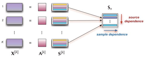
IVA for multi-dataset analysis and the two key signal properties available in addition to HOS: sample dependence and dependence among sources within a source component matrix S_n

$${\mathbf{x}}^{[k]}(v)={\mathbf{A}}^{[k]}{\mathbf{s}}^{[k]}(v),1\le k\le K,1\le v\le V$$ (2)

where A^[k] ∈ ℝ^N×N, k = 1, …, K are invertible matrices and the source estimates are u^[k](v) = W^[k]x^[k](v). We define the nth source component vector (SCV) s_n as

$${\mathbf{s}}_n(v)={\left[s_n^{[1]}(v),s_n^{[2]}(v),\dots ,s_n^{[K]}(v)\right]}^{\top }\in {ℝ}^K$$ (3)

by concatenating the nth source from each of the K datasets, or similarly, define the source component matrix (SCM) S_n shown in Figure 1, through concatenation of the nth row of each S^[k]. The SCV takes into account sample dependence through the inclusion of index v in its notation—or simply when we write it as an SCM—and more importantly, since it is defined using corresponding sources across all K datasets, this is the term that accounts for the dependence across the datasets and the cost function is defined with respect to the SCV.

IVA thus maximizes independence across the SCVs by minimizing the mutual information rate [10]

$${\mathcal{I}}_r^{\text{IVA}}(\mathcal{W})=\sum _{n=1}^N{H}_r({\mathbf{u}}_n)-\sum _{k=1}^{K}log\left|det\left({\mathbf{W}}^{[k]}\right)\right|-C$$ (4)

$$=\sum _{n=1}^N\left(\sum _{k=1}^K{H}_r(u_n^{[k]})-{\mathcal{I}}_r({\mathbf{u}}_n)\right)-\sum _{k=1}^{K}log\left|det\left({\mathbf{W}}^{[k]}\right)\right|-C,$$ (5)

where the (differential) entropy rate denoted with subscript r is H_r(u_n) = lim_v→∞ [H[u_n(1), …, u_n(v)]/v] and the entropy H (u_n) = −E{log p_sn(u)}. Here, 𝒲 refers to the block diagonal KN×KN weight matrix with N×N matrices W^[k] as the diagonal blocks.

Since entropy rate measures the per sample density of the average uncertainty of a random process, minimization of (4) makes use of both HOS—through the minimization of missing information, entropy—and sample dependence by making the samples easier to predict by increasing sample dependence, i.e., decreasing the entropy rate. The term log | det W^[k]| acts as a regularization term preserving the volume across the directions of source estimation and results when we use the Jacobian for H_r(u). The role of diversity across datasets in IVA is evident if we study (5), as here the second term ${\sum }_{n=1}^N{\mathcal{I}}_r({\mathbf{u}}_n)$ accounts for the dependence within the components of an SCV. While the goal is to decrease the entropy rate for each SCV to minimize the mutual information rate and increase independence, this term has negative sign, indicating the need to increase mutual information within the components of an SCV, to make use of the dependence—whenever it exists. Without this second term, the IVA cost is the same as the sum of K separate ICAs performed on each dataset. Hence, IVA makes use of dependence across the datasets, when it exists, and only for the components for which it does exist. Thus this is not a requirement in general. In any case, the goal in a joint decomposition is taking advantage of the diversity among the datasets. Finally, when we have a single dataset, K = 1, the SCV u_n = u_n is a scalar quantity and IVA reduces to ICA.

For a given set of observations, one can write the likelihood and study the performance of the ICA/IVA estimator using maximum likelihood theory. The Fisher information matrix tells us how informative the observations are for the estimation of the demixing matrix and the conditions that guarantee the positive definiteness of the Fisher Information matrix—since it is a covariance matrix—also give the identification conditions for the ICA/IVA model. It is shown that, both for ICA and IVA, it is the SOS that determine identifiability—for a detailed discussion of the conditions see [10], [41]. In the case of IVA, one can identify i.i.d. Gaussian sources as long as they are correlated across the datasets, an important result that underlines the advantages of exploiting all available diversity when jointly decomposing multiple datasets.

B. Two examples—Algorithm choice and role of diversity

We demonstrate the role of diversity in performance of ICA and IVA and how different types of diversity can be taken into account with two examples. First, consider the separation of two linearly mixed sources using ICA, an i.i.d. source drawn from a generalized Gaussian distribution (GGD) and a second source, a first-order autoregressive (AR) process generated by an i.i.d. Gaussian process (v) such that s(v) = as(v − 1) + ν(v). For a GGD, the probability density function (pdf) is Gaussian for shape parameter β = 1, super-Gaussian when β ∈ (0, 1) and sub-Gaussian when β > 1. Thus, β quantifies the role of HOS, and the AR coefficient, a of sample dependence, with increasing role of HOS as β moves away from 1 and sample dependence as a moves away from 0. In Figure 2(a), we plot the induced Cramér-Rao lower bound (CRLB) using the interference-to-signal-ratio (ISR) as in [10]. The results are shown for 1000 samples and 500 independent runs. First note that for finite CRLB, it suffices for one of the sources to have sample correlation—nonzero a—when both are Gaussian. The widely referenced and repeated condition for the real case that says “with ICA one can identify only a single Gaussian,” hence is true only when sample dependence is not taken into account—or is absent in that the samples are i.i.d., which rarely is the case in practice. In the same figure, we also show the performance of three different ICA algorithms, efficient variant of FastICA (EFICA) [42], WASOBI [40], and entropy rate bound minimization (ERBM) [43], [44]. EFICA takes only HOS into account and uses a parametric GGD model, hence is a good match for the sources in this example. WASOBI makes use of only second-order statistics, sample correlation, and can approach the CRLB for stationary AR sources. Finally, ERBM uses a flexible density matching mechanism based on entropy maximization and also accounts for sample dependence through an invertible filter model. As shown in Figure 2(a), only ERBM can account for the two types of diversity that exists in this example, HOS and sample dependence. Since it is a simple, computationally attractive, joint diagonalization algorithm, WASOBI provides more competitive performance when sources are correlated Gaussians (β = 1) and EFICA can only approach the bound for the case when there is no sample correlation. While we observe that the exact density match as in the case of EFICA provides the best performance for the i.i.d. case, the flexible ERBM can approach the bound as well. The properties of EFICA, WASOBI and many others can be studied under the mutual information rate minimization, and hence ML, umbrella [10], [45].

Fig. 2.

Two examples to demonstrate the role of diversity for (a) ICA (HOS and sample dependence); and (b) IVA (HOS, sample dependence, and source dependence) with respect to the induced CRLB. For both examples, note the improvement in performance as the role of HOS increases, i.e., as shape parameter β moves away from 1, as sample dependence, i.e., the value of AR coefficient a, increases, and in the case of IVA, as shown in (b), as source dependence measured by correlation across datasets ρ increases.

In the second example, shown in Figure 2(b), we demonstrate the role of diversity for IVA, where in addition to HOS and sample dependence—quantified by β and a respectively as in the previous case—we also have correlation among sources ρ. Source correlation is introduced for the first pair of sources that come from a multivariate GGD, and the second pair is a first-order vector AR process with a diagonal coefficient matrix aI. As observed in the figure, with the inclusion of each new type of diversity, the performance improves (the CRLB/normalized ISR decreases). The CRLB is finite—hence the model is identifiable, even when all sources are i.i.d. Gaussians as long as there is correlation across the pair of Gaussian sources, i.e., sources within an SCV.

With IVA as well, depending on the algorithm chosen, multiple types of diversity can be taken into account, however algorithm design is more challenging due to the multivariate nature of sources. Both IVA-GGD that uses a fixed shape parameter from a number of candidates [46] and its adaptive variant IVA-A-GGD [47] can take HOS into account, but like EFICA, they are based on the simple GGD density model, which is limited to unimodal and symmetric distributions. IVA-ERBM [48] uses a more flexible density model that includes symmetric, skewed, unimodal, and bimodal marginals for the multivariate density model and also incorporates sample dependence. In the figure we also show the performance of three IVA algorithms, IVA with the multivariate Gaussian model (IVA-G) [9], IVA-A-GGD, [47], and IVA-ERBM [48]. IVA-G can only account for SOS, sample and source correlation, while IVA-A-GGD takes HOS into account and is a good match for the SCVs in this example. However, IVA-ERBM provides the best performance as it accounts for all three types of diversity available for this problem, at the expense of highest computational complexity, as expected.

C. CCA, MCCA, and IVA

IVA is intimately related to CCA [49] and its generalization to multiple datasets, MCCA [22]. IVA generalizes both to the case where not only SOS but all-order statistics can be taken into account and where the demixing matrix is not constrained to be orthogonal. CCA is most likely the oldest method that enables inference from two datasets by letting them interact in a symmetric manner, i.e., by treating the two datasets similarly. It has been widely applied in economics, biomedical data analysis, medical imaging, meteorology, and signal processing among others [50]. Using the notation presented in Section II-A, CCA finds pairs of weighting vectors ${\mathbf{w}}_n^{[1]}$ and ${\mathbf{w}}_n^{[2]}$ to transform x^[1] and x^[2] such that the normalized correlation between their transformations $u_n^{[1]}={\left({\mathbf{w}}_n^{[1]}\right)}^{\top }{\mathbf{x}}^{[1]}$ and $u_n^{[2]}={\left({\mathbf{w}}_n^{[2]}\right)}^{\top }{\mathbf{x}}^{[2]}$ is maximized.

In [22], a number of extensions of CCA to multiple datasets, all termed multi-set CCA, are described and presented under a common umbrella. They can be introduced by using the SCV definition in (3) as follows. In order to maximize the correlation among the K datasets, we search for vectors ${\mathbf{w}}_n^{[k]}$, k = 1, …, K such that the correlation within an SCV ${\mathbf{u}}_n={\left[u_n^{[1]},u_n^{[2]},\dots ,u_n^{[K]}\right]}^{\top }\in {ℝ}^K$ where $u_n^{[k]}={\left({\mathbf{w}}_n^{[k]}\right)}^{\top }{\mathbf{x}}^{[k]}$, is maximized. This is achieved through a deflationary approach where one first estimates ${\mathbf{w}}_n^{[k]}$ for k = 1, …, K, and then proceeds to the estimation of ${\mathbf{w}}_{n+1}^{[k]}$ for k = 1, …, K such that ${\mathbf{w}}_n^{[k]}$ is orthogonal to ${\mathbf{w}}_{n+1}^{[k]}$, thus resulting in matrices W^[k] that are orthogonal.

There are five metrics introduced in [22] where each has the goal of increasing the correlation within an SCV estimate, u_n, by moving the SCV correlation matrix ${\mathbf{R}}_n=E\{{\mathbf{u}}_n{\mathbf{u}}_n^{\top }\}$ close to being singular, i.e., increasing the spread of the eigenvalues. Examples include MAXVAR that maximizes the largest eigenvalue of R_n and GENVAR that minimizes the product of eigenvalues, i.e., the determinant, of R_n. The GENVAR cost provides the connection with IVA. If we were to assume that a multivariate Gaussian model is used for the SCV, thus only taking second-order statistics into account and ignoring sample dependence by assuming i.i.d. samples, we can substitute the entropy of a multivariate Gaussian for the nth SCV $(1/2)log\left[{(2\pi e)}^K{\mathrm{\Pi }}_{k=1}^K{\lambda }_n^{[k]}\right]$ where ${\lambda }_n^{[k]}$, k = 1, …, K are the eigenvalues of R_n into (4). Given that in MCCA, the demixing matrices W^[k] are constrained to be orthogonal the last term in (4) disappears and hence the IVA cost reduces to the minimization of the product of eigenvalues of R_n under a given constraint, such as on the sum of the eigenvalues.

Thus, IVA generalizes MCCA and justifies the use of GEN-VAR within a maximum likelihood framework, additionally, when IVA algorithms are designed using a richer class of models for the multivariate pdfs as in [48], then one can fully incorporate HOS, as well as sample dependence. As such, IVA is readily applicable to all the problems for which MCCA has proved useful, and in addition, can take HOS across multiple datasets into account, allowing for better use of available statistical information.

D. Application of ICA, MCCA, and IVA to joint data analysis and fusion

ICA as well as CCA/MCCA enable joint BSS and have been used for multivariate data fusion and analysis. In this section, we provide a brief overview of these applications and address how IVA provides an effective solution for multi-set data analysis as already demonstrated with a number of convincing examples, and can be also used for multi-modal data fusion through the tIVA model we introduce in Section III. In the discussion, we differentiate between multi-set data analysis—also called fusion in certain contexts—and multimodal data fusion and address the two separately next.

Multi-set data refers to multiple datasets that are essentially of the same type and dimension such as video or image sequences from multiple channels—e.g., RGB channels or multi-spectra—or from multiple views, medical imaging data such as fMRI or EEG data collected from multiple subjects, with multiple conditions or tasks, and remote sensing data at different time instances, spectral bands, angles, or polarizations. One way to analyze multiple datasets within a blind source separation framework is by defining a single dataset through simple concatenation of these datasets and then performing a single ICA on this new single dataset. Two such models have proven useful, especially with application to medical image analysis and fusion: the Group ICA model that concatenates multiple datasets in the vertical dimension followed by a principal component analysis (PCA) step [33], [51] and the jICA model that performs this concatenation horizontally such that each dataset is stacked next to each other [1], [2]. Group ICA model has been typically used for analysis of data from multiple subjects [33], [51], [52]—hence for multi-set data—and jICA for multi-modal data fusion. However, depending on the nature of the data and the task at hand, there are examples of different use for each model as in [12], [53]. Another way to perform multi-set analysis is to directly make use of the IVA model shown in Figure 1 as it allows for full interaction of multiple datasets without additional constraints such as the definition of a common “group subspace” as in Group ICA or a common mixing matrix as in the jICA model. IVA has been successfully used in multi-set data analysis. Examples include multisubject fMRI analysis [54]–[56], study of brain dynamics in rest data [57], enhancing of steady-state visual evoked potentials (SSVEP) for detection [58] among others. Similarly, MCCA has been used for multi-set analysis, for analysis of multi-subject fMRI data [23], [24], and Landsat Thematic Mapper data with spectral bands over a number of years [25].

Multi-modal data, on the other hand, refers to information collected about the same phenomenon using different types of modalities or sensors, where the modalities provide complementary information and thus joint analysis of such data is expected to provide a more complete and informative view about the task at hand. Examples include functional medical imaging data such as EEG and fMRI data that report on distinct aspects of brain function, EEG by recording electrical activity through electrodes placed on the scalp and fMRI by imaging the brain hemodynamic response. In addition, one can fuse structural MRI and/or diffusion tensor imaging data along with functional data to incorporate structure information, or one can also look at associations with genetic information such as single nucleotide polymorphism (SNP) data. Similarly, in remote sensing, optical and radar imagery provide complementary information, where the synthetic radar aperture systems complement the information optical sensors provide for horizontal objects bypassing the limitations on time-of-day and atmospheric conditions for the optical sensors. This is our main focus in this article, fusion of data from multiple modalities where the datasets are complementary to each other, though, typically of different nature, size, and resolution.

Feature-based fusion of multi-modal data

Since our focus is on multi-modal fusion with the goal of letting the modalities fully interact in a symmetric manner, there are a number of challenges that need to be overcome. A major one stems from the fact that the nature of data from various modalities is inherently different and the best way to treat them equally for true fusion is thus not evident, and in addition, their dimensionality and resolutions differ. One effective way to overcome both of these challenges is to define a set of multivariate features such that most of the variability in the data is still preserved, i.e., these are not higher level features that are simple summary statistics, but are still multivariate. By generating such features, one can establish a dimension of coherence that enables the creation of a link among the multi-modal data through this common dimension.

This is the approach that has been used in the fusion of medical imaging data with the jICA approach [1], [2] and in MCCA [20], as well as their variations, such as parallel ICA [11], linked ICA [59], and MCCA + jICA [60]. A natural example is the use of features extracted for multiple subjects where the subject profiles/covariations provide the common dimension over which the modalities are linked. For data acquired during an event-related task, these can be task-related contrast images for fMRI data, event-related potentials for EEG, and when there is no task, e.g., when working with rest data, fractional amplitude of low frequency fluctuations could provide the features for fMRI and EEG. For structural MRI when fused with functional data, making use of segmented gray matter images is meaningful since the activity would be expected to be connected to gray matter only. Besides subjects, the common dimension can be defined using different conditions, trials, or time instances at which the multimodal data are acquired. In all of these cases, we can look for underlying components that have similar (dependent) covariations across the multivariate features. We provide specific examples in [21], but first, in the next section, define the two models based on ICA and IVA to effectively link such datasets.

III. The Joint ICA and Transposed IVA models for multi-modal fusion and their properties

Given K ≥ 2 datasets that have a common dimension N, we define two models: the jICA and the tIVA models to fuse multi-modal feature data, or multiple datasets with at least one dimension of coherence. We show the two models in Figure 3. An application example would be multivariate features extracted from fMRI, EEG, sMRI, and SNP data (or a combination of those) for N subjects where the common dimension is the subjects and associations across modalities are achieved through subject covariations, i.e., profiles. The jICA model is introduced in [2] where it is applied to construct chronometry of auditory oddball target detection from EEG and fMRI data in healthy subjects and is implemented in the Fusion ICA Toolbox (FIT, http://mialab.mrn.org/software/fit/) for application to medical imaging data. The tIVA model generalizes the model introduced in [20] where MCCA is used to maximize profile correlations across modalities to the case where HOS and dataset dependences are also taken into account. Next, we first provide an overview of the two methods and then discuss the choice of an algorithm for each, emphasizing the role of diversity, and consider the problem of order selection and validation.

Fig. 3.

Two models for multi-modal data fusion for multiple datasets—shown for K = 2. Note the change in the role of sources and mixing matrix columns for the profiles and components.

A. Comparison of the two models

In order to compare the two models shown in Figure 3, we first establish the terminology, especially in reference to components vs profiles. As an example, consider a case where we have multivariate features extracted from N different subjects and the connection among the two datasets is established by subject covariations. Let the multi-modality datasets be formed by stacking features from the two groups once after another, then if we are looking for differences between the groups then the subject covariations correspond to the profile that indicates a difference between the groups as in the example case considered in Figure 4. Or, alternatively if we are studying a single group and looking at similar components, these would be profiles that exhibit small variations among its entries.

Fig. 4.

Generative model for the simulations.

By transposing the datasets in tIVA, the role of samples and observations is reversed with respect to jICA, if we define the matrices as the number of observations by samples. In addition, while in jICA the independent sources correspond to components, e.g., fMRI spatial maps, ERP or sMRI components, that are linked across a common profile, in tIVA, the independent sources become the profiles, i.e., the subject covariations. Hence, we prefer to use profile and component as shown in Figure 3 within the context of fusion, which, depending on the model used, can refer to either sources—that are independent—or columns of mixing matrix/matrices, which are close to being orthogonal even when not constrained by the algorithm as in FastICA. This is due to the role of the last term log |detW^[k]| in the the ICA/IVA cost (4) that acts as a regularizer, which is maximum for orthogonal W and minimum when any two rows of W are co-linear. Below we summarize the properties of the profiles and components, which play an important role in the decision of how to choose one model over another. For jICA in Figure 3, the associated components are

• constrained to have the same profile across modalities, and

• independent among themselves;

while the profiles—a single set for all modalities—are close to being orthogonal among themselves. For tIVA, however, it is the profiles that are

• maximally dependent across the modalities (for corresponding profiles), and

• independent among themselves within a modality

while the components are close to being orthogonal within a modality.

Since even for a representation at the feature-level, the nature of datasets is still typically very different, the link is established by finding components for which the covariations across the datasets are similar. In the case of the jICA model, we constrain these to be exactly the same across the modalities, and for tIVA, maximally statistically dependent, as in this case, a given profile across the modalities corresponds to a single SCV defined in Section 3. IVA makes use of dependence that exists across the datasets when achieving the decomposition hence making the tIVA model more flexible than jICA. Thus, when there are components that are common across only a subset of the datasets, IVA will be able to identify those while the performance of jICA will suffer as there is a strong mismatch to the underlying model for jICA. Similarly, when the strength (correlation) of connections among components across the modalities are significantly different, tIVA will again outperform jICA. However when the noise and uncertainty is an important concern, an approach that imposes strong constraints like jICA can be preferable as we demonstrate with examples. The tall nature of the data matrices in Figure 3 makes it clear that IVA needs to be performed after a dimension reduction step where the selected order is less than N, a topic we address in Section III-C. Because for tIVA, the samples refer to N, e.g., number of subjects rather than the samples within features as in jICA, the tIVA model requires a significant number of samples N to have sufficient statistical power.

These differences in the properties of the profiles and components imply additional considerations. An important application for both of these models is the identification of biomarkers between groups of subjects—or conditions. In these cases, the subject dimension N includes subjects from M classes such that $N={\sum }_{m=1}^M{N}_m$ and components that report on differences across groups of subjects can be identified by detecting differences in subject covariations—values in the profile coefficients for corresponding groups—through a statistical test, such as a simple t-test. When applied to differences between two groups as in [11], [24] the profiles assume a step type response, and one can identify only one such component with tIVA and up to two with jICA as sample size tends to infinity. When the goal is identifying differences in more than two groups of subjects, then both models show limitations as neither orthogonality nor independence can be satisfied for such profiles, and certain extensions need to be considered, which we discuss in Section V. However, it is important to note that such considerations are of concern when we have very large sample sizes, and hence will depend on the number of samples, e.g., subjects available for the study.

B. Algorithm choice

Besides model choice, the algorithm used for achieving the independent decomposition plays an important role in the final results. For example, all of the results we are aware of and are discussed in [21], use the Infomax algorithm in their jICA implementations. As in the case of ICA of fMRI data, Infomax has been the first algorithm applied to fusion of medical imaging data, and has been the default choice in the toolbox implementing the method, FIT. This might explain the bias in its choice in the literature. However, Infomax uses a fixed nonlinearity, one that is matched to super-Gaussian sources, and hence Infomax source estimates tend to be all highly super-Gaussian, thus also sparse. This is also the case for FastICA, in particular with the most commonly used kurtosis nonlinearity. An algorithm like EBM that uses a flexible density model, or like ERBM that takes multiple types of diversity into account makes better use of the statistical properties that are available and finds sources from a wider range of distributions leading to better maximization of independence as we also demonstrate with examples in this paper. In addition, in the jICA model, associated components are assumed to come from the same pdf, thus use of an ICA algorithm with a more flexible source pdf is more desirable since it allows for a richer model for the joint pdf.

For the tIVA model, the only fusion examples reported to date have used CCA and MCCA, and primarily the MAXVAR cost, which yields robust estimates, but of course as with all other MCCA solutions, can only take SOS into account, and thus can only find uncorrelated profiles not those that are independent within a dataset like tIVA. With IVA, as discussed in Section II-B, multiple types of diversity can be taken into account depending on the algorithm chosen such as HOS and source dependence using IVA-GGD [46] or its adaptive version [47], source and sample dependence in addition to HOS using IVA-ERBM [48] at the expense of increased computational complexity.

With the tIVA model, since the independent sources correspond to the profiles, use of HOS and of diversity across the datasets provides multiple advantages. Thanks to this diversity, one can identify profiles that are i.i.d. Gaussians as long as they are dependent across the datasets, and that is the case one is interested in for fusion since these correspond to components—columns of mixing matrix in tIVA—that are linked across the multi-modal datasets. In addition, a profile that corresponds to a difference between two groups will assume a step-like shape, hence will have a distribution where HOS and sample dependence play an important role.

Finally, the “approximately orthogonal” property for the demixing matrices discussed in Section III can be made more strict, and can be imposed during the estimation as is the case in FastICA and EFICA algorithms, and also for MCCA, which can be used for tIVA model. In this case, for the given number of (finite) samples, the orthogonality property will be more closely satisfied for the profiles in the jICA model and the components in the tIVA model, and this determines the nature of multiple profiles or components estimated by each, just like the independence assumptions as discussed in Section III. A cautionary remark here is regarding the role of whitening of the data prior to ICA, as sometimes mistakenly noted, this whitening is not sufficient to limit the search space for W to orthogonal matrices. This becomes true only when the sample size tends to infinity, or when it is imposed in the estimation procedure as in FastICA and MCCA. Thus, it is important to remember that IVA with the multivariate Gaussian model, IVA-G, and MCCA using GENVAR are equivalent only when the demixing is constrained to be orthogonal for IVA-G, and otherwise IVA-G includes a wider search space than MCCA with GENVAR. Orthogonality provides certain advantages such as enabling easier density matching, however its advantages can be preserved through a decoupling procedure [61] without constraining W to be orthogonal, and is implemented in a number ICA and IVA algorithms including EBM, ERBM, IVA-GGD, and IVA-ERBM.

C. Order selection and validation

As in most source separation problems, determining the order of signal subspace M where we let x = A_xs_x + n_x with x, n_x ∈ ℝ^N and s_x ∈ ℝ^M, M ≥ N, and performing the fusion in the signal subspace improves the generalization ability, and hence provides robustness. This model also justifies the use of noiseless ICA model for the mixing as the noise is removed prior to fusion. For jICA, since it is performed after concatenation of multi-modal data, we treat the resulting $N\times {\sum }_{k=1}^K{N}_k$ dimensional dataset as one, one can directly proceed with order selection as in ICA of overdetermined problems, see e.g., [23]. The development in Section II-A allows us to work directly within the maximum likelihood framework through the equivalence of entropy rate and maximum likelihood by the asymptotic equipartition property and to make use of the desirable large sample properties of maximum likelihood. The formulation for order selection in [62] assumes a multivariate Gaussian model for s_x and the penalty function to balance the increasing likelihood with complexity can be chosen from a number of options such as Akaike’s information criterion (AIC) [63], Bayesian information criterion (BIC) [64], or the minimum description length (MDL) [65]. When writing the likelihood term in this formulation however, the inherent assumption is that the samples are i.i.d., which is not true for most signals. For example in fMRI data, there is inherent spatial smoothness due to the point spread function of the scanner. The hemodynamic process also has some inherent smoothness. Furthermore, smoothing is a common preprocessing step used to suppress the high frequency noise in the fMRI data and to minimize the impact of spatial variability among subjects. Similarly in EEG data, there is strong temporal correlation among the samples. As a result, the order is usually highly overestimated when these criteria are used directly as in [62] and the samples are not as informative due to sample dependence. One practical solution to the problem uses entropy rate to measure independence among samples and determines a downsampling depth for the samples [66]. In [67], the problem is addressed by jointly estimating the downsampling depth and the order. However downsampling decreases the effective sample size thus limiting the ability of maximum likelihood estimator to achieve its optimality conditions. A more recent approach [68] addresses this issue by using a formulation based on entropy rate, i.e., by directly modeling the sample dependence structure to write the likelihood. In addition, the consistency of the MDL/BIC criterion is established for the given formulation.

In all of these cases, one typically uses singular value decomposition (SVD) to perform PCA and reduce the dimensionality to the order suggested by the selected information-theoretic criterion. Using SVD rather than eigenvalue decomposition allows handling the two models, transposed and regular, i.e., tIVA and IVA, similarly, and obviously the singular values for both X ∈ ℝ^N×V and X^T are the same. Hovewer, when determining order of multiple datasets as in tIVA or the regular IVA model, it is important to remember that one is usually interested in identifying the dimensionality of the subspace of components that are common across the datasets, rather than those that are specific to each. Hence, keeping the largest variance for each dataset—the common practice in most order selection steps—might not yield the desired solution. A number of possibilities exist to address this problem among which we can include being conservative with the PCA step and keeping most of the variability in the data is one, or using joint analysis approaches such as CCA [69], MCCA/IVA, and higher-order generalized SVD [70] to explore the nature of correlation/dependence across the datasets. An important point in such analyses relates to the effect of sample size. As studied in [71] for CCA, i.e., for two datasets, when the number of samples is smaller than the sum of the ranks of two data matrices, the estimated canonical correlation coefficients can be estimated as unity. For the tIVA model since typically N ≪ V_k, all pairwise canonical correlation coefficient estimates are expected to be close to 1 and hence uninformative. The solution proposed in [72] for two datasets uses a linear mixing model as in [62] and uses a reduced rank version of a hypothesis test to address this issue, and hence is a promising solution for this scenario as well.

One practical approach to determine the order has been to test the stability of the results for different orders and choose a number within a range where it is stable [18], [24]. This has been mostly an empirical study, where the goal has been to see whether the estimated components provide significant change across orders measured by simple correlation type measures. For validation, one can take advantage of the ML framework and evaluate conditional likelihood given various estimators for different models considered as in [73], and when looking at group differences, increase in the detected differences, the results of pairwise t-statistics is another possibility as we discuss in [21] within the context of the selected application, fusion of medical imaging data.

IV. Simulation Examples

In this section, we present two sets of simulations to demonstrate scenarios where tIVA might be preferable over jICA and vice versa. The generative model used in the simulations is demonstrated in Figure 4 where for each dataset, we generate 10 sources each with 500 i.i.d. samples drawn from a zero mean Laplacian distribution with a standard deviation of 4, which are linearly mixed using a 50×10 matrix where the first column has a step-type characteristics to simulate a difference between the two groups—a control and a patient group—each with 25 samples (subjects). The remaining nine columns of the mixing matrix are i.i.d. samples from a Gaussian distribution. The mixing matrix column with the step response, a₁ ∈ ℝ⁵⁰, establishes the link among the datasets, i.e., results in the component that demonstrates the group difference. Thus we have a₁ = c + n₁ and a_i = n_i for i = 2, …, 10. Here, c is the step profile shown in Figure 4, and the standard deviation σ_ni of the zero-mean Gaussian noise for n_i, i = 2, …, 10 is adjusted such that it matches the standard deviation of a₁ for each case we consider. The number of samples that correspond to subjects is chosen as 50, a relatively low value, to consider a case similar to the examples with real data. The first simulation example shown in Figure 5 considers two datasets, and a second one with results given in Figure 6, fusion of three datasets. We tested the performance of jICA using EBM, and tIVA using IVA-G and MCCA using MAXVAR and GENVAR for three datasets, and using IVA-G and CCA for two datasets. Since the sources are Laplacian, jICA-Infomax is expected to perform similarly, and for tIVA we used only second-order algorithms available for two datasets as the total number of samples (subjects) is relatively small, only 50. Identifiability condition for tIVA-G/CCA/MCCA is satisfied for only one component (profile), while for jICA for all as the sources are independent Laplacians. For jICA, the datasets are simply concatenated and dimension is reduced to 10—the true order—yielding X ∈ ℝ^10×1000 for the case with two datasets and X ∈ ℝ^10×1500 for three datasets, and for tIVA, each dataset is reduced in dimension resulting in (X^[k])^⊤ ∈ ℝ^10×50. Results are the average of 100 independent runs. In the figures, we show the average correlation of the estimated component whose estimated profile had the highest average t-statistic (between the groups of 25 subjects each) and the original component which had the step-type profile.

Fig. 5.

Estimation performance for the common component with two datasets as (a) the height of the step in the profile changes, (b) the noise level added to the step profile changes, and (c) the number of subjects increases with a fixed noise and height level.

Fig. 6.

Estimation performance for the common component with three datasets as the connection of one dataset—the height of the step—decreases in terms of (a) t-statistic for the most significant component, (b) correlation of the most significant component to the original, and (c) when the connection of one dataset is kept low and the number of subjects increases.

In the first set of simulations, we consider two datasets and control the correlation (link) between the two datasets by either changing the height of the step in c or by keeping the height constant (at 1.5) and changing σ_n1. Hence, we study the performance of the two models when the underlying common structure between the two datasets becomes weaker as well as when it is strong but the level of noise increases. For the results shown in Figure 5(a), σ_n1 = 0.3 and the height of the step is changed as 0.1 + 0.1k where k = 0, …, 14,—resulting in correlation values in the range [0.1,1]—and for the results shown in Figure 5(b), we have σ_n1 = 0.1 + 0.1k where k = 0, …, 10—resulting in correlation values [0.3, 1]. For the first case, when the connection becomes weaker due to the change in the underlying structure—step height—tIVA-G provides better performance than jICA. For the second case, jICA performs better as the noise level increases since the underlying structure is strong—the step size is kept constant at 1.5—and jICA tends to average out the effect of noise. It is also worthwhile noting the degradation in performance with CCA compared to IVA-G due to the orthogonality constraint for CCA that limits the search space for the optimal demixing matrices. Additionally, as the step size decreases, the mixing matrices become closer to being orthogonal resulting in an initial improved performance for CCA. In Figure 5(c), we show the change in performance as the number of subjects increase for σ_n1 = 0.3 and identical step responses of 1.5. The results demonstrate the advantages for tIVA model as the number of subjects increase.

The second set of simulations considers three datasets, again with one common component across all three. We first study the effect of decreasing correlation for one dataset by decreasing the step height for this one component while the step for the other two are kept constant at 1, and σ_n1 = 0.3. In Figure 6, we show trends in the t-statistic and the estimation performance measured with correlation of the estimate to the original for the components for which the step size is altered. A couple of points need to be emphasized. First, note that the significance for the component in terms of group difference estimated by jICA tends to increase while the estimation of the component itself—its correlation with the original—starts to decrease. On the other hand, the tIVA model yields reliable estimates for the t-statistics and correlation values for the for the component that has the weak connection to the other two as shown in Figure 6(a). For the other two components whose step sizes are kept constant—results not shown,—however, jICA in general yields higher values and closer to the truth for the t-statistic than the tIVA solutions but its correlation for these two components is lower than those of tIVA. In this example, since the demixing matrix is closer to being orthogonal—especially when the step height decreases,—the performances of tMCCA-MAXVAR and tMMCA-GENVAR are slightly better than tIVA-G, as these are more efficient solutions to the problem, especially in the case of MCCA-MAXVAR algorithm. Finally, in Figure 6(c), the step height for the third modality is kept at 0.3 while the other two are 1 for σ_n1 = 0.3 as the number of samples (subjects) is increased. The increasing sample size improves the performance of all approaches including jICA, though as expected, its performance suffers for the estimation of the component with weak correlation as shown, and its estimation for the components with the stronger link is higher—around .75—while those of tIVA solutions are close to 1—results not shown. Finally, the estimates for the t-statistics for both jICA and tIVA solutions are reliable for the components with the strong link, and with tIVA for the weak component as well while it is over-estimated with jICA—again, figures not shown.

V. Discussion

In this paper, we considered techniques based on blind source separation for data-driven fusion of multiple sets of data, with focus on two models for multi-modal fusion, the jICA and the tIVA models. The jICA model has been introduced for fusion of medical imaging data, and tIVA extends the model introduced using MCCA—again within the context of medical imaging—to incorporate HOS. However, both of these are general models that enable multivariate fusion in a symmetric manner and can be applied to fusion of multi-modal data in fields outside medical imaging through appropriate definition of the features. Even though the focus of the current paper is on the fusion of multi-modal data, both models can be used for fusion/analysis of multi-set data as well, which is addressed in Section II-B in terms of role and use of diversity in ICA and IVA decompositions. Depending on the problem, the multi-set data can be concatenated horizontally as in the jICA model, or vertically as in Group ICA [51], or we can use IVA as in the tIVA model, or without the transposed version, as originally defined in (2).

On algorithm choice

By specifically focusing on two separate models for multi-modal fusion, our goal has been to review their properties and elucidate the key considerations in their application. Along with the model choice, other decisions such as algorithm to use and the order of the signal subspace, all have an impact on the final results. For example, for the jICA model, which is now quite widely used, Infomax has been the main algorithm of choice in all the publications we have cited—the only exception is [74] which uses COMBI, a combination of EFICA and WASOBI algorithms [75]. Infomax is also the default algorithm in the Fusion ICA Toolbox [76], which implements the method. However, as we show, the use of a more flexible ICA algorithm such as EBM significantly improves the performance. Since in jICA, concatenation of multiple datasets leads to a richer distribution than that of each modality alone, the underlying distribution of the common components cannot be effectively captured by the Infomax algorithm, which uses a simple fixed nonlinearity. In addition, since this nonlinearity provides a match to sources that are super-Gaussian, it naturally emphasizes estimation of sources that are more sparse.

Sparsity vs independence

The discussion on the usefulness of either of the two assumptions, independence versus sparsity, in data-driven analysis has been a topic of discussion in various fields including the analysis of fMRI data [77], [78]. Dictionary learning, for example, can be used to achieve fusion by promoting sparsity [79]. However, dictionary learning, like most matrix decomposition methods requires the definition of additional constraints with appropriate weighting factors to enable uniqueness and solutions that are interpretable. On the other hand, for most BSS decompositions and ICA, we can obtain unique solutions subject to rather mild conditions, and without the need to define additional constraints. In addition, estimates obtained using ICA or IVA are naturally smooth and hence physically easy to interpret. This has been another reason for the desirability of solutions based on BSS. It has been this simplicity that contributed to the popularity of ICA, especially with the introduction of the Infomax algorithm [34]—especially when implemented using relative/natural gradient updates [80], [81]—along with the FastICA [35] algorithm, that they could be applied to many problems easily. However, it is important to note that there are now a number of ICA algorithms to choose from, and by selecting one that uses a flexible nonlinearity like EBM, we can better make use of HOS to maximize independence. We can also take additional types of diversity such as sample dependence into account to better maximize independence and approach the induced CRLB as demonstrated by Example 2(a). As we demonstrate in [21], for multi-modal data fusion, the use of a flexible algorithm like EBM better optimizes the ICA criterion—as measured through mutual information—and leads to estimates that are easier to interpret, suggesting that independence is indeed a very useful objective.

Importance of diversity, ML framework, and order selection

When performing data fusion, a key source of diversity is dependence across datasets as shown for IVA in Example 2(b). Working within the ML framework enables performance evaluations by studying performance of a given algorithm against the CRLB as shown in these examples, and provides additional advantages such as performance evaluations using conditional likelihoods as in [73]. Perhaps more importantly, working within ML framework allows us incorporate model order selection naturally into the analysis through use of information-theoretic criteria. Order selection plays an important role in the performance of the final fusion results, and also presents an effective means to perform exploratory analysis of multimodal data by enabling us to determine orders of both specific and common signal subspaces across multiple datasets. As we note in Section III-C, for the sample poor case, the estimation of signal subspace order is a difficult problem, one that requires special care. This problem is recently addressed for two datasets when performing CCA [72], and has provided meaningful results for the cases considered. Its extension to multiple datasets along with the use of methods such as higher-order generalized SVD [70] hold much promise for the exploratory analysis of multi-modal data since the order of common signal subspaces provides a direct measure of the link that exists across the datasets. A reliable method for determining the order can guide the choice of a model, features to use, and in what form, among others.

As we have noted, there are already a number of extensions of the jICA model discussed here. While extensions are always useful, we should first clearly understand the properties of a given model and the variables that affect its performance to make sure we are making full use of the advantages the model has to offer. This has been our main objective in this article, to provide such a guidance. Obviously the cases one might consider in simulated examples are very broad, and we have chosen to concentrate on examples that parallel the problem represented with the example that uses real data in the accompanying paper [21] where the goal is identifying components (biomarkers) that correspond to group differences. When searching for components that reflect differences in more than two groups for example, the limitations posed by the models such as independence and orthogonality of the components or profiles will require extensions to the ICA and IVA such that they enable decompositions of independent subspaces rather than independent components as in [82]–[85]. Another important case arises when the goal is trying to find underlying components that help explain the data rather than identifying group differences, as in the study of multimodal data from only a healthy group, which was the original application for the introduction of jICA [2]. For this problem, tIVA model is particularly attractive as the profiles in this case correspond to sources and can be identified even when they are Gaussian as long as they are dependent across the subjects—and, these are the sources that yield the components of interest given by the columns of the mixing matrices. In all the simulation examples as well as the results with real data [21], we have used second-order IVA algorithms, IVA-G and MCCA since the examples included cases with low sample sizes. But as shown in the simulations, the tIVA model has advantages when the number of samples—subjects, in the cases we considered—increases. When the number of samples increases, using IVA algorithms that take HOS statistics into account such as IVA-GGD [41], [47], or one that takes both sample dependence and HOS into account as in IVA-ERBM [48] will be more desirable.

Our paper, we hope, highlights the main issues that need to be taken into account in the application of fusion methods based on BSS, which has offered an attractive solution to the problem. By addressing the main issues and trade-offs involved in their use, our goal has been not only to provide guidance but also to emphasize topics of research that will significantly extend the power of these methods. Even though our focus has been on two models, which provide useful decompositions of data that are also easy to interpret, most of the issues we addressed arise in the application of other data-driven models, in particular those based on matrix and tensor decompositions, and hence would also benefit from a closer look of the topics we addressed such as order selection for multiple sets of data.

Biographies

Tülay Adali (S’89–M’93–SM’98–F’09) received the Ph.D. degree in Electrical Engineering from North Carolina State University, Raleigh, NC, USA, in 1992 and joined the faculty at the University of Maryland Baltimore County (UMBC), Baltimore, MD, USA, the same year. She is currently a Distinguished University Professor in the Department of Computer Science and Electrical Engineering at UMBC. Prof. Adali assisted in the organization of a number of international conferences and workshops including the IEEE International Conference on Acoustics, Speech, and Signal Processing (ICASSP), the IEEE International Workshop on Neural Networks for Signal Processing (NNSP), and the IEEE International Workshop on Machine Learning for Signal Processing (MLSP). She was the General Co-Chair, NNSP (2001–2003); Technical Chair, MLSP (2004–2008); Program Co-Chair, MLSP (2008, 2009, and 2014), 2009 International Conference on Independent Component Analysis and Source Separation; Publicity Chair, ICASSP (2000 and 2005); and Publications Co-Chair, ICASSP 2008. She is Technical Program Co-Chair for ICASSP 2017 And Special Sessions Co-Chair for ICASSP 2018.

Prof. Adali chaired the IEEE Signal Processing Society (SPS) MLSP Technical Committee (2003–2005, 2011–2013), served on the SPS Conference Board (1998–2006), and the Bio Imaging and Signal Processing Technical Committee (2004–2007). She was an Associate Editor for IEEE Transactions on Signal Processing (2003–2006), IEEE Transactions on Biomedical Engineering (2007–2013), IEEE Journal of Selected Areas in Signal Processing (2010–2013), and Elsevier Signal Processing Journal (2007–2010). She is currently serving on the Editorial Boards of the Proceedings of the IEEE and Journal of Signal Processing Systems for Signal, Image, and Video Technology, and is a member of the IEEE Signal Processing Theory and Methods Technical Committee.

Prof. Adali is a Fellow of the IEEE and the AIMBE, a Fulbright Scholar, recipient of a 2010 IEEE Signal Processing Society Best Paper Award, 2013 University System of Maryland Regents’ Award for Research, and an NSF CAREER Award. She was an IEEE Signal Processing Society Distinguished Lecturer for 2012 and 2013. Her research interests are in the areas of statistical signal processing, machine learning for signal processing, and biomedical data analysis.

Yuri Levin-Schwartz received the B.S. degree in physics and the B.A. degree in mathematics, both from Brandeis University, Waltham, Massachusetts, in 2012. He is currently a Ph.D. candidate at the Machine Learning for Signal Processing Lab, University of Maryland, Baltimore County. His research interests include blind source separation, machine learning, statistical signal processing, and biomedical data analysis.

Vince D. Calhoun (S’91–M’02–SM’06–’F13) received a bachelor’s degree in Electrical Engineering from the University of Kansas, Lawrence, Kansas, in 1991, master’s degrees in Biomedical Engineering and Information Systems from Johns Hopkins University, Baltimore, in 1993 and 1996, respectively, and the Ph.D. degree in electrical engineering from the University of Maryland Baltimore County, Baltimore, in 2002. He worked as a research engineer in the psychiatric neuroimaging laboratory at Johns Hopkins from 1993 until 2002. He then served as the director of medical image analysis at the Olin Neuropsychiatry Research Center and as an associate professor at Yale University.

Dr. Calhoun is currently Executive Science Officer and Director of Image Analysis and MR Research at the Mind Research Network and is a Distinguished Professor in the Departments of Electrical and Computer Engineering (primary), Biology, Computer Science, Neurosciences, and Psychiatry at the University of New Mexico. He is the author of more than 400 full journal articles and over 500 technical reports, abstracts and conference proceedings. Much of his career has been spent on the development of data driven approaches for the analysis of brain imaging data. He has won over $85 million in NSF and NIH grants on the incorporation of prior information into ICA for functional magnetic resonance imaging, data fusion of multimodal imaging and genetics data, and the identification of biomarkers for disease, and leads a P20 COBRE center grant on multimodal imaging of schizophrenia, bipolar disorder, and major depression.

Dr. Calhoun is a fellow of the IEEE, The Association for the Advancement of Science, The American Institute of Biomedical and Medical Engineers, and the International Society of Magnetic Resonance in Medicine. He is also a member and regularly attends the Organization for Human Brain Mapping, the International Society for Magnetic Resonance in Medicine, the International Congress on Schizophrenia Research, and the American College of Neuropsychopharmacology. He is also a regular grant reviewer for NIH and NSF. He has organized workshops and special sessions at multiple conferences. He is currently chair of the IEEE Machine Learning for Signal Processing (MLSP) technical committee. He is a reviewer for many journals is on the editorial board of the Brain Connectivity and Neuroimage journals and serves as Associate Editor for Journal of Neuroscience Methods and several other journals.

References

- 1.Calhoun VD, Adali T. Feature-based fusion of medical imaging data. IEEE Trans Info Technology in Biomedicine. 2009 Sep;13(5):711–720. doi: 10.1109/TITB.2008.923773. [DOI] [PMC free article] [PubMed] [Google Scholar]
- 2.Calhoun VD, Adali T, Pearlson GD, Kiehl KA. Neuronal chronometry of target detection: Fusion of hemodynamic and event-related potential data. NeuroImage. 2006 Apr;30(2):544–553. doi: 10.1016/j.neuroimage.2005.08.060. [DOI] [PubMed] [Google Scholar]
- 3.Comon P. Independent component analysis, A new concept? Signal Processing. 1994;36(9):287–314. [Google Scholar]
- 4.Comon P, Jutten C. Handbook of Blind Source Separation: Indepedent Component Analysis and Applications. Academic Press; 2010. [Google Scholar]
- 5.Sui J, Adali T, Yu Q, Chen J, Calhoun V. A review of multivariate methods for multimodal fusion of brain imaging data. Journal of Neuroscience Methods. 2012;204:68–81. doi: 10.1016/j.jneumeth.2011.10.031. [DOI] [PMC free article] [PubMed] [Google Scholar]
- 6.Adali T, Haykin S. Adaptive Signal Processing: Next Generation Solutions. Hoboken, New Jersey: Wiley Interscience; 2010. [Google Scholar]
- 7.Hyvärinen A, Karhunen J, Oja E. Independent Component Analysis. New York, NY: Wiley; 2001. [Google Scholar]
- 8.Kim T, Lee I, Lee T-W. Independent vector analysis: Definition and algorithms. Proc 40th Asilomar Conf Signals, Systems, Comput. 2006:1393–1396. [Google Scholar]
- 9.Anderson M, Li XL, Adali T. Joint blind source separation with multivariate Gaussian model: Algorithms and performance analysis. IEEE Trans Signal Processing. 2012 Apr;60(4):2049–2055. [Google Scholar]
- 10.Adali T, Anderson M, Fu GS. Diversity in independent component and vector analyses: Identifiability, algorithms, and applications in medical imaging. IEEE Signal Proc Mag. 2014 May;31(3):18–33. [Google Scholar]
- 11.Calhoun VD, Liu J, Adali T. A review of group ICA for fMRI data and ICA for joint inference of imaging, genetic, and ERP data. NeuroImage. 2009 Mar;45(1):S163–S172. doi: 10.1016/j.neuroimage.2008.10.057. [DOI] [PMC free article] [PubMed] [Google Scholar]
- 12.Eichele T, Calhoun VD, Moosmann M, Specht K, Jongsma ML, Quiroga RQ, Nordby H, Hugdahl K. Unmixing concurrent EEG-fMRI with parallel independent component analysis. International Journal of Psychophysiology. 2008;67(3):222–234. doi: 10.1016/j.ijpsycho.2007.04.010. [DOI] [PMC free article] [PubMed] [Google Scholar]
- 13.Specht K, Zahn R, Willmes K, Weis S, Holtel C, Krause BJ, Herzog H, Huber W. Joint independent component analysis of structural and functional images reveals complex patterns of functional reorganisation in stroke aphasia. NeuroImage. 2009;47:2057–2063. doi: 10.1016/j.neuroimage.2009.06.011. [DOI] [PubMed] [Google Scholar]
- 14.Mangalathu-Arumana J, Beardsley S, Liebenthal E. Within-subject joint independent component analysis of simultaneous fMRI/ERP in an auditory oddball paradigm. NeuroImage. 2012;60:2247–2257. doi: 10.1016/j.neuroimage.2012.02.030. [DOI] [PMC free article] [PubMed] [Google Scholar]
- 15.Mijovic B, Vanderperren K, Novitskiy N, Vanrumste B, Stiers P, Bergh BV, Lagae L, Sunaert S, Wagemans J, Huffel SV, Vos MD. The “why” and “how” of JointICA: Results from a visual detection task. NeuroImage. 2012;60:1171–1185. doi: 10.1016/j.neuroimage.2012.01.063. [DOI] [PubMed] [Google Scholar]
- 16.Magtibay K, Beheshti M, Foomany FH, Balasundaram K, Masse PLS, Asta J, Zamiri N, Jaffray DA, Nanthakumar K, Krishnan S, Umapathy K. Fusion of structural and functional cardiac magnetic resonance imaging data for studying ventricular fibrillation. Proc IEEE Int Conf Eng in Medicine and Biology Spciety. 2014:5579–5582. doi: 10.1109/EMBC.2014.6944891. [DOI] [PubMed] [Google Scholar]
- 17.Swinnen W, Hunyadi B, Acar E, Huffel SV, Vos MD. Incorporating higher dimensionality in joint decomposition of eeg and fmri incorporating higher dimensionality in joint decomposition of eeg and fmri incorporating higher dimensionality in joint decomposition of eeg and fmri. Proc. European Signal Process. Conf. (EUSIPCO); Lisbon, Portugal. September 2014. [Google Scholar]
- 18.Ramezani M, Abolmaesumi P, Marble K, Trang H, Johnsrude I. Fusion analysis of functional mri data for classification of individuals based on patterns of activation. Brain Imaging and Behavior. 2014:1–13. doi: 10.1007/s11682-014-9292-1. [DOI] [PubMed] [Google Scholar]
- 19.Imani F, Ramezani M, Nouranian S, Gibson E, Khojaste A, Gaed M, Moussa M, Gomez J, Romagnoli C, MLM, Chang S, Fenster A, Siemens DR, Ward A, Mousavi P, Abolmaesumi P. Ultrasound-based characterization of prostate cancer using joint independent component analysis. IEEE Trans Biomedical Eng. 2015 doi: 10.1109/TBME.2015.2404300. to appear. [DOI] [PubMed] [Google Scholar]
- 20.Correa NM, Li YO, Adali T, Calhoun VD. Canonical correlation analysis for feature-based fusion of biomedical imaging modalities and its application to detection of associative networks in schizophrenia. IEEE J Selected Topics in Signal Processing. 2009;2(6):998–1007. doi: 10.1109/JSTSP.2008.2008265. [DOI] [PMC free article] [PubMed] [Google Scholar]
- 21.Adali T, Levin-Schwartz Y, Calhoun VD. Multi-modal data fusion using source separation: Application to medical imaging. Proc IEEE. 2015 doi: 10.1109/JPROC.2015.2461624. same issue. [DOI] [PMC free article] [PubMed] [Google Scholar]
- 22.Kettenring JR. Canonical analysis of several sets of variables. Biometrika. 1971 Dec;58(3):433–451. [Google Scholar]
- 23.Li Y-O, Wang W, Adali T, Calhoun VD. Joint blind source separation by multi-set canonical correlation analysis. IEEE Trans Signal Processing. 2009 doi: 10.1109/TSP.2009.2021636. [DOI] [PMC free article] [PubMed] [Google Scholar]
- 24.Correa N, Adali T, Calhoun VD. Canonical correlation analysis for data fusion and group inferences: Examining applications of medical imaging data. IEEE Signal Processing Magazine. 2010 Jul;27(4):39–50. doi: 10.1109/MSP.2010.936725. [DOI] [PMC free article] [PubMed] [Google Scholar]
- 25.Nielsen AA. Multiset canonical correlations analysis and multi-spectral, truly multitemporal remote sensing data. IEEE Trans Image Process. 2002 Mar;11(3):293–305. doi: 10.1109/83.988962. [DOI] [PubMed] [Google Scholar]
- 26.Moreau E, Adali T. Blind Identification and Separation of Complex-valued Signals. London, UK and Hoboken, NJ: ISTE and Wiley; 2013. [Google Scholar]
- 27.Cardoso JF, Souloumiac A. Blind beamforming for non-Gaussian signals. IEE Proc Radar Signal Processing. 1993 Dec;140(6):362–370. [Google Scholar]
- 28.Li X-L, Adali T, Anderson M. Joint blind source separation by generalized joint diagonalization of cumulant matrices. Signal Processing. 2011 Oct;91(10):2314–2322. [Google Scholar]
- 29.Chabriel G, Kleinsteuber M, Moreau E, Shen H, Tichavský P, Yeredor A. Joint matrices decompositions and blind source separation. a survey of methods, identification and applications. IEEE Signal Proc Mag. 2014 May;31(3):34–43. [Google Scholar]
- 30.Li X-L, Anderson M, Adali T. Second and higher-order correlation analysis of multiple multidimensional variables by joint diagonalization. Proc. 2010 Conf. Latent Variable Analysis and Independent Component Analysis (LVA/ICA); St. Malo, France. Sept. 2010. [Google Scholar]
- 31.Adali T, Li H, Novey M, Cardoso JF. Complex ICA using nonlinear functions. IEEE Trans Signal Processing. 2008 Sep;56(9):4356–4544. [Google Scholar]
- 32.Adali T, Schreier PJ, Scharf LL. Complex-valued signal processing: The proper way to deal with impropriety. IEEE Trans Signal Processing. 2011 Nov;59(11):5101–5123. [Google Scholar]
- 33.Calhoun VD, Adali T. Multisubject independent component analysis of fMRI: A decade of intrinsic networks, default mode, and neurodiagnostic discovery. IEEE Reviews in Biomedical Engineering. 2012 Aug;5:60–73. doi: 10.1109/RBME.2012.2211076. [DOI] [PMC free article] [PubMed] [Google Scholar]
- 34.Bell A, Sejnowski T. An information maximization approach to blind separation and blind deconvolution. Neural Computation. 1995 Nov;7(6):1129–1159. doi: 10.1162/neco.1995.7.6.1129. [DOI] [PubMed] [Google Scholar]
- 35.Hyvärinen A. Fast and robust fixed-point algorithms for independent component analysis. IEEE Trans Neural Networks. 1999 May;10(3):626–634. doi: 10.1109/72.761722. [DOI] [PubMed] [Google Scholar]
- 36.Boscolo R, Pan H, Roychowdhury V. Independent component analysis based on nonparametric density estimation. IEEE Trans Neural Networks. 2004 Jan;15(1):55–65. doi: 10.1109/tnn.2003.820667. [DOI] [PubMed] [Google Scholar]
- 37.Pham D, Garat P. Blind separation of mixtures of independent sources through a quasi maximum likelihood approach. IEEE Trans Signal Processing. 1997 Jul;45(7):1712–1725. [Google Scholar]
- 38.Tong L, Liu RW, Soon VC, Huang YF. Indeterminacy and identifiability of blind identification. IEEE Trans Circuits Syst. 1991 May;38(5):499–509. [Google Scholar]
- 39.Belouchrani A, Abed-Meraim K, Cardoso JF, Moulines E. A blind source separation technique using second-order statistics. IEEE Trans Signal Processing. 1997 Feb;45(2):434–444. [Google Scholar]
- 40.Yeredor A. Blind separation of Gaussian sources via second-order statistics with asymptotically optimal weighting. IEEE Signal Proc Letts. 2000 Jul;7(7):197–200. [Google Scholar]
- 41.Anderson M. PhD dissertation. University of Maryland Baltimore County; May, 2013. Independent vector analysis: Theory, algorithms, and applications. [Google Scholar]
- 42.Koldovský Z, Tichavský P, Oja E. Efficient variant of algorithm FastICA for independent component analysis attaining the Cramér-Rao lower bound. IEEE Trans Neural Networks. 2006 Sep;17(5):1265–1277. doi: 10.1109/TNN.2006.875991. [DOI] [PubMed] [Google Scholar]
- 43.Li X-L, Adali T. Blind spatiotemporal separation of second and/or higher-order correlated sources by entropy rate minimization. Proc. IEEE Int. Conf. Acoust., Speech, Signal Processing (ICASSP); Dallas, TX. March 2010; pp. 1934–1937. [Google Scholar]
- 44.Fu GS, Phlypo R, Anderson M, Li X-L, Adali T. Blind source separation by entropy rate minimization. IEEE Trans Signal Processing. 2014 Aug;62(16):4245–4255. [Google Scholar]
- 45.Yeredor A. Blind separation of Gaussian sources with general covariance structures: Bounds and optimal estimation. IEEE Trans Signal Processing. 2010 Oct;58(10):5057–5068. [Google Scholar]
- 46.Anderson M, Fu G-S, Phlypo R, Adali T. Independent vector analysis, the Kotz distribution, and performance bounds. Proc. IEEE Int. Conf. Acoust., Speech Signal Process. (ICASSP); Vancouver, BC. May 2013; pp. 3243–3247. [Google Scholar]
- 47.Boukouvalas Z, Fu G-S, Adali T. An efficient multivariate generalized Gaussian distribution estimator: Application to IVA. Proc. Conf. Information Sciences and Systems; Baltimore, MD. March 2015. [Google Scholar]
- 48.Fu G-S, Anderson M, Adali T. Independent vector analysis by entropy rate bound minimization. Proc. Conf. on Info. Sciences and Systems (CISS); Baltimore, MD. March 2015; pp. 1–6. [Google Scholar]
- 49.Hotelling H. Relations between two sets of variates. Biometrika. 1936 Dec;28(3/4):321–377. [Google Scholar]
- 50.Borga M. Canonical correlation a tutorial. 2001 www.imt.liu.se/people/magnus/cca/tutorial/
- 51.Calhoun VD, Adali T, Pekar JJ, Pearlson GD. A method for making group inferences from functional MRI data using independent component analysis. Human Brain Mapping. 2001 Nov;14(1):140–151. doi: 10.1002/hbm.1048. [DOI] [PMC free article] [PubMed] [Google Scholar]
- 52.Allen EA, Erhardt E, Wei Y, Eichele T, Calhoun VD. Capturing inter-subject variability with group independent component analysis of fMRI data: a simulation study. NeuroImage. 2012;59:4141–4159. doi: 10.1016/j.neuroimage.2011.10.010. [DOI] [PMC free article] [PubMed] [Google Scholar]
- 53.Mijovic B, Vos MD, Vanderperren K, Machilsen B, Sunaert S, Huffel SV, Wagemans J. The dynamics of contour integration: A simultaneous EEG–fMRI study. NeuroImage. 2014;88:10–21. doi: 10.1016/j.neuroimage.2013.11.032. [DOI] [PubMed] [Google Scholar]
- 54.Lee JH, Lee TW, Jolesz FA, Yoo SS. Independent vector analysis (IVA): Multivariate approach for fMRI group study. NeuroImage. 2008;40(1):86–109. doi: 10.1016/j.neuroimage.2007.11.019. [DOI] [PubMed] [Google Scholar]
- 55.Laney J, Westlake K, Woytowicz E, Ma S, Adali T. Capturing subject variability in fMRI data: A graph theoretical analysis of GICA vs IVA. Journal of Neuroscience Methods. 2014 doi: 10.1016/j.jneumeth.2015.03.019. submitted. [DOI] [PMC free article] [PubMed] [Google Scholar]
- 56.Michael A, Anderson M, Miller R, Adali T, Calhoun VD. Preserving subject variability in group fMRI analysis: Performance evaluation of GICA vs IVA. Frontiers Syst Neuroscience. 2014 doi: 10.3389/fnsys.2014.00106. to appear. [DOI] [PMC free article] [PubMed] [Google Scholar]
- 57.Ma S, Calhoun VD, Phlypo R, Adali T. Dynamic changes of spatial functional network connectivity in healthy individuals and schizophrenia patients using independent vector analysis. NeuroImage. 2014 Apr;90:196–206. doi: 10.1016/j.neuroimage.2013.12.063. [DOI] [PMC free article] [PubMed] [Google Scholar]
- 58.Emge D, Vialette F, Dreyfus G, Adali T. Independent vector analysis for SSVEP signal enhancement. Proc. Conf. Information Sciences and Systems; Baltimore, MD. 2015. [Google Scholar]
- 59.Groves AR, Beckmann CF, Smith SM, Woolrich MW. Linked independent component analysis for multimodal data fusion. NeuroImage. 2011;54(3):2198–2217. doi: 10.1016/j.neuroimage.2010.09.073. [Online]. Available: http://dx.doi.org/10.1016/j.neuroimage.2010.09.073. [DOI] [PubMed] [Google Scholar]
- 60.Sui J, He H, Pearlson GD, Adali T, Kiehl KA, Yu Q, Clark VP, Castro E, White T, Mueller BA, Ho BC, Andreasen NC, Calhoun VD. Three-way (N-way) fusion of brain imaging data based on mCCA+jICA and its application to discriminating schizophrenia. NeuroImage. 2013 Feb;66:119–132. doi: 10.1016/j.neuroimage.2012.10.051. [DOI] [PMC free article] [PubMed] [Google Scholar]
- 61.Anderson M, Li X-L, Rodriguez PA, Adali T. An effective decoupling method for matrix optimization and its application to the ICA problem. Proc. IEEE Int. Conf. Acoust., Speech, Signal Processing (ICASSP); Kyoto, Japan. March 2012; pp. 1885–1888. [Google Scholar]
- 62.Wax M, Kailath T. Detection of signals by information theoretic criteria. IEEE Trans Acoustics, Speech, and Signal Processing. 1985 Apr;33(2):387–392. [Google Scholar]
- 63.Akaike H. A new look at statistical model identification. IEEE Trans Auto Control. 1974;19:716–723. [Google Scholar]
- 64.Schwarz GE. Estimating the dimensions of a model. Ann Stats. 1978;6(2):461–464. [Google Scholar]
- 65.Rissanen J. Modeling by the shortest data description. Automatica. 1978;14:465–471. [Google Scholar]
- 66.Li YO, Adali T, Calhoun VD. Estimating the number of independent components for fMRI data. Human Brain Mapping. 2007 Nov;28(11):1251–1266. doi: 10.1002/hbm.20359. [DOI] [PMC free article] [PubMed] [Google Scholar]
- 67.Li X-L, Ma S, Calhoun VD, Adali T. Order detection for fmri analysis: Joint estimation of downsampling depth and order by information theoretic criteria. Proc. IEEE Int. Symp., Biomedical Imaging: From Nano to Macro; April 2011; pp. 1019–1022. [Google Scholar]
- 68.Fu GS, Anderson M, Adali T. Likelihood estimators for dependent samples and their application to order selection. IEEE Trans Signal Processing. 2014 Aug;62(16):4237–4244. [Google Scholar]
- 69.Zhang QT, Wong KM. Information theoretic criteria for the determination of the number of signals in spatially correlated noise. IEEE Trans Signal Processing. 1993 Apr;41(4):1652–1663. [Google Scholar]
- 70.Ponnapalli SP, Saunders MA, Loan CFV, Alter O. A higher-order generalized singular value decomposition for comparison of global mRNA expression from multiple organisms. PLoS ONE. 2011 Dec; doi: 10.1371/journal.pone.0028072. [DOI] [PMC free article] [PubMed] [Google Scholar]
- 71.Pezeshki A, Scharf LL, Azimi-Sadjadi MR, Lundberg M. Empirical canonical correlation analysis in subspaces. Proc 38th Asilomar Conf on Signals, Systems and Computers. 2004;1:994–997. [Google Scholar]
- 72.Song Y, Schreier P, Roseveare NJ. Determining the number of correlated signals between two data sets using PCA-CCA when sample support is extremely small. Proc. IEEE Int. Conf. Acoust., Speech Signal Process. (ICASSP); Brisbane, Australia. April 2015. [Google Scholar]
- 73.Engemann DA, Gramfort A. Automated model selection in covariance estimation and spatial whitening of meg and eeg signals. NeuroImage. 2015 doi: 10.1016/j.neuroimage.2014.12.040. to appear. [DOI] [PubMed] [Google Scholar]
- 74.Sui J, Pearlson G, Caprihan A, Adali T, Kiehl KA, Liu J, Yamamoto J, Calhoun VD. Discriminating schizophrenia and bipolar disorder by fusing fMRI and DTI in a multimodal CCA+ joint ICA model. NeuroImage. 2011;57(3):839–855. doi: 10.1016/j.neuroimage.2011.05.055. [DOI] [PMC free article] [PubMed] [Google Scholar]
- 75.Tichavský P, Koldovský Z, Doron E, Yeredor A, Gómez-Herrero G. Blind signal separation by combining two ica algorithms: HOS-based EFICA and time structure-based WASOBI. Proc. European Signal Process. Conf. (EUSIPCO); Florence, Italy. 2006. [Google Scholar]
- 76.Fusion ICA toolbox. http://mialab.mrn.org/software/fit/. [Online]. Available: http://mialab.mrn.org/software/fit/
- 77.Daubechies I, Roussos E, Takerkarta S, Benharrosha M, Goldenb C, D’Ardennea K, Richtera W, Cohena JD, Haxbyaw J. Independent component analysis for brain fMRI does not select for independence. Proc National Academy of Sciences. 2009 Jun;106(26):10 415–10 422. doi: 10.1073/pnas.0903525106. [DOI] [PMC free article] [PubMed] [Google Scholar]
- 78.Calhoun VD, Potluru VK, Phlypo R, Silva RF, Pearlmutter BA, Caprihan A, Plis SM, Adali T. Independent component analysis for brain fMRI does indeed select for maximal independence. PLoS ONE. 2013;8(8):e73309. doi: 10.1371/journal.pone.0073309. [DOI] [PMC free article] [PubMed] [Google Scholar]
- 79.Remazani M, Marble K, Trang H, Johnsrude IS, Abolmaesumi P. Joint sparse representation of brain activity patterns in multi-task fMRI data. IEEE Trans Med Imaging. 2015 Jan;34(1):2–12. doi: 10.1109/TMI.2014.2340816. [DOI] [PubMed] [Google Scholar]
- 80.Amari S-I, Cichocki A, Yang HH. A new learning algorithm for blind signal separation. In: Touretzky DS, Mozer MC, Hasselmo ME, editors. Advances in Neural Information Processing Systems, December 1995. Vol. 8. The MIT Press; 1996. pp. 757–763. [Google Scholar]
- 81.Cardoso JF, Laheld B. Equivariant adaptive source separation. IEEE Trans Signal Processing. 1996 Dec;44(12):3017–3030. [Google Scholar]
- 82.Lahat D, Cardoso JF, Messer H. Second-order multidimensional ICA: Performance analysis. IEEE Trans Signal Processing. 2012 Sep;60(9):4598–4610. [Google Scholar]
- 83.Hyvärinen A, Hoyer PO, Inko M. Topographic independent component analysis. Neural Computation. 2001 Jul;13(7):1527–1558. doi: 10.1162/089976601750264992. [DOI] [PubMed] [Google Scholar]
- 84.Cardoso JF. Multidimensional independent component analysis. Proc. IEEE Int. Conf. Acoust., Speech, Signal Processing (ICASSP); Seattle, WA. May 1998; pp. 1941–1944. [Google Scholar]
- 85.Silva R, Pils S, Adali T, Calhoun VD. Multidataset independent subspace analysis extends independent vector analysis. Proc. IEEE Int. Conf. on Image Proc; Paris, France. Oct. 2014; [DOI] [PMC free article] [PubMed] [Google Scholar]