Computational Image Analysis Reveals Intrinsic Multigenerational Differences between Anterior and Posterior Cerebral Cortex Neural Progenitor Cells

Summary

Time-lapse microscopy can capture patterns of development through multiple divisions for an entire clone of proliferating cells. Images are taken every few minutes over many days, generating data too vast to process completely by hand. Computational analysis of this data can benefit from occasional human guidance. Here we combine improved automated algorithms with minimized human validation to produce fully corrected segmentation, tracking, and lineaging results with dramatic reduction in effort. A web-based viewer provides access to data and results. The improved approach allows efficient analysis of large numbers of clones. Using this method, we studied populations of progenitor cells derived from the anterior and posterior embryonic mouse cerebral cortex, each growing in a standardized culture environment. Progenitors from the anterior cortex were smaller, less motile, and produced smaller clones compared to those from the posterior cortex, demonstrating cell-intrinsic differences that may contribute to the areal organization of the cerebral cortex.

Graphical Abstract

Highlights

• •Open-source automated software designed to track stem/progenitor clones in time-lapse movies
• •Software tools for easy data validation and visualization greatly improve efficiency
• •Lineage tree reconstruction from hundreds of embryonic mouse forebrain clones
• •Intrinsic differences in progenitor behavior from anterior/posterior cerebral cortex

Cohen, Temple, and colleagues describe new techniques for segmenting, tracking, and lineaging stem and progenitor cells through multiple rounds of division in time-lapse phase contrast images. Manual validation is combined with automated analysis, minimizing effort to correct any errors. Progenitors from anterior and posterior mouse cerebral cortex cultured identically exhibited differences in behavior, indicating early encoding of cortex area identity.

Introduction

Time-lapse microscopy enables the patterns of development, cellular motion, and morphology to be observed and captured for clones of proliferating cells. Phase contrast microscopy allows image capture at a temporal resolution sufficient for accurate tracking through multiple rounds of cell division in a label-free manner. By integrating appropriate incubation, live cell development can be imaged over a period of days or even weeks. An experiment can produce 350 gigabyte (GB) of image data and there is a pressing need for efficient analytical computational tools.

In general, humans are better able to correctly identify and track cells than the best available software, but manual tracking is prohibitively slow. In order to efficiently analyze time-lapse phase image sequences of proliferating cells, the best current approach is to combine human visual capabilities with automated image analysis algorithms.

Human validation is essential to correct errors produced by the automated programs, which fall into three classes: segmentation, tracking, and lineaging errors. Segmentation identifies individual cells in each image. A segmentation error has occurred if a cell is not correctly detected. Tracking is the process by which objects are followed from one frame to another. Tracking errors occur when segmentation results identifying different cells are associated on the same track. Lineaging errors occur when the parent-daughter relationships are incorrectly identified. Our algorithms allow some segmentation errors, such as when a cell is obscured for a single frame, but all tracking and lineaging errors must be corrected. Human validation corrects these errors and the goal is to minimize the user corrections required.

The clones used in this study were derived from neural progenitor cells (NPCs) extracted from the embryonic mouse cerebral cortex. NPCs include neural stem cells and more restricted progenitor cells. The cortex performs numerous functions, integrating sensory information, thought, and memory with appropriate behavioral responses. Different cortical functions are achieved through areal specializations. For example, the visual cortex is concerned with processing information derived from the retina, while the motor cortex drives movement via subcortical connections to the spinal cord. The visual cortex arises in the posterior region of the embryonic telencephalon, and the motor cortex arises from the anterior region. How these two distinct areas develop differently from each other is an important question in developmental neurobiology. It is possible that the anterior and posterior NPCs are intrinsically similar and rely on the presence of growth factor gradients (O’Leary et al., 2007) to direct their output. Alternatively, the growth factor gradients might instill cell-intrinsic changes in the NPCs to alter their behavior. In order to discern these two possibilities, we need to study the growth of anterior and posterior NPCs exposed to the same environment, which can only be done ex vivo. The hypothesis we tested is that anterior and posterior cortical NPCs are intrinsically different, reflected in different lineage outputs and behaviors when cultured in a standardized environment.

Results

E12.5 mouse anterior or posterior cortical NPCs were plated in a 24 well plate at clonal density in serum-free culture medium, with images captured every 5 min for over 4 days. Image data gathered in three separate experiments was initially segmented, tracked, and lineaged, according to the process outlined in Figure 1. These initial segmentation and tracking algorithms have been applied in a number of recent applications (Chenouard et al., 2014, Cohen et al., 2009, Cohen et al., 2010, Mankowski et al., 2014, Winter et al., 2011, Winter et al., 2012). We developed a new segmentation algorithm that uses lineage information to automatically improve segmentation and tracking accuracy in a step referred to as “post-lineage refinement”. The post-lineage refinement uses the parent-daughter information that is challenging for current machine vision approaches (Seungil et al., 2011), but relatively fast and easy for a human to identify. The segmentation and tracking results were then automatically refined from the corrected lineage information with human observers correcting any remaining segmentation and tracking errors interactively. All of the validation was done using a program called Lineage Editing and Validation (LEVER) (Winter et al., 2011). LEVER allows a user to visualize the lineage tree together with the segmentation and tracking results. The results are color coded in order to make errors as easy to identify as possible. Manual edits and the automatic corrections are logged and counted to determine the error rates of the different algorithms. All of the software and algorithms are available free and open source as detailed below.

Figure 1.

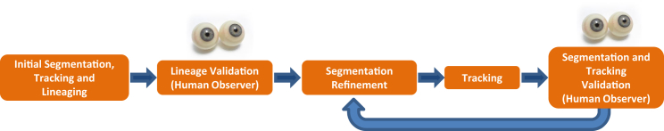
Overview of Approach

Starting with an initial segmentation, cells are tracked through the image data and a lineage is obtained. The parent-daughter relationships in the lineage are validated by the human observer. The validated lineage is then used to refine the segmentation and tracking under supervision. This refine and then validate process is repeated for each image, achieving a significant reduction in the segmentation error rate.

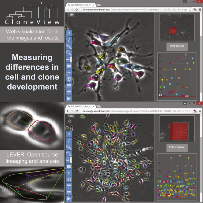
Figure 2 shows a montage of all 160 lineage trees, a total of 10,644 cells and 1,585,104 segmentations. Movie S1 shows a sample movie for a posterior clone with segmentation and tracking overlaying the image data in the left panel and the lineage tree in the right panel. Our web-based visualization program CloneView provides an interactive way to explore the data and results. Figure 3 shows a screen shot of the CloneView program with a summary listing the clones in one window and one image frame with segmentation and tracking results overlaid in the other window. All of the image data, together with all segmentation and tracking results, are available through our web-based tool called CloneView. CloneView runs on any computer that supports a modern web browser with no software to download. CloneView is available at http://n2t.net/ark:/87918/d91591.

Figure 2.

Lineage Trees for the 78 Clones of Posterior Progenitor Cells and 82 Clones of Anterior Progenitor Cells Analyzed Here

Note the differences in lineage tree shape within and between regions.

Figure 3.

All of the Images Together with the Results Can Be Browsed from an Easy to Use Web Application Called CloneView

CloneView lists summary information for each clone (left) and allows the images to be explored, with segmentation and tracking optionally overlaid (right), CloneView: http://n2t.net/ark:/87918/d91591.

The initial segmentation algorithm error rate of 8.1% represents all the segmentation errors including both the automatic corrections generated by the post-lineage refinement (6.4%) and the user-provided manual corrections (1.7%). This represents a 79% reduction in segmentation error rate compared to the initial segmentation. This initial segmentation incorporates our previous development of stem cell segmentation algorithms (Mankowski et al., 2014, Wait et al., 2014, Winter et al., 2011). The tracking error rate was 1%. The total error rate, calculated from the number of edit operations required to fully correct the segmentation, tracking, and lineaging errors, was 1.3%. Once validated, we can extract features such as cell lifespan, location, and size, enabling quantification of the cell-cycle time, motion, and morphology for individual cells, across clones and broken down by generation. The analysis of this feature data reveals significant differences in the patterns of development between anterior and posterior cerebral cortical NPCs.

The Lineage Tree Is Used to Refine the Underlying Segmentation

Of all the tasks required for this analysis, segmentation, or delineation of individual cells in each image frame is the most challenging and error prone. Even human observers can find it difficult to establish the correct number of cells in a close group from a single image. When the number of cells has been correctly established, clustering models that incorporate morphological characteristics of the cells, together with temporal information from the tracking, reliably separate the foreground pixels into individual cells.

We begin with an initial segmentation algorithm originally developed for phase contrast images of retinal stem cells (Cohen et al., 2010) and applied previously to neural stem cells (Winter et al., 2012). Modified versions of this segmentation algorithm have been applied to oligodendrocyte precursors (Cohen et al., 2010) and hematopoietic stem cells (Mankowski et al., 2014). Following the initial segmentation, we apply a Multitemporal Assocation Tracking (MAT) algorithm. MAT was originally developed for tracking organelle transport (Chenouard et al., 2014, Winter et al., 2012) and was found to be effective for tracking stem cells (Winter et al., 2011), reducing the error rates compared to previous approaches (Al-Kofahi et al., 2006, Cohen et al., 2010) by 86%. Inference approaches (Papadimitriou and Steiglitz, 1998, Pearl, 1988) automatically improve the lineage tree, using the tracking graph together with constraints that cells do not appear or disappear between frames except across the imaging border, unless there is a mitosis or cell death.

We integrate human validation with the automated processing tasks because for our purposes the tracking and lineaging results must be 100% correct. Using the fully automated approach still significantly reduces error rates, for applications that can accept some errors. Movie S2 shows an image sequence of a developing clone with both automated (yellow boxes) and manual (red boxes) edits indicated. For this clone, using the inference-improved lineage to refine the initial segmentation produces an error rate of 1.5%. Using the human-corrected lineage reduces the error rate to 1.1%. Including the lineage and tracking errors and results, the total error rate for fully correcting the clone was 0.9%. This clone can also be explored using CloneView, http://n2t.net/ark:/87918/d91591?1.

An advantage of the new segmentation method is that once the number of cells in the frame is established, as described above, other important characteristics such as cell morphology can be incorporated to improve accuracy. Figure 4 shows the results of refining an existing segmentation for two different scenarios. Figure 4A shows three cells initially segmented as one. Figure 4B shows the result using the watershed transform (Gonzales et al., 2009) to estimate the number of cells. Once the correct number of cells has been established using information from the tracking and lineaging algorithms, the foreground pixels need to be separated into the individual cells. When the cells have a circular morphology (Mankowski et al., 2014), a k-means clustering algorithm works well; this is not the case for the NPCs shown in Figure 4C. For elliptically shaped cells, a Gaussian mixture model (GMM) clustering on the spatial locations of the foreground pixels incorporates the morphology of the cells and finds the correct separation, as shown in Figure 4D. A second example with two touching cells is shown in Figures 4E–4H.

Figure 4.

Resegmentation Using a Known Number of Cells

Segmentation examples (top and bottom) starting from initial segmentations that incorrectly identify the number of cells (A and E). We use the lineage tree to correctly establish the number of cells, improving over traditional methods such as the watershed transform (B and F). Partitioning of the pixels into cells (C and G) is improved by using an elliptical shape model (D and H). The scale bars represent 10 μm, CloneView top: http://n2t.net/ark:/87918/d91591?3 and bottom: http://n2t.net/ark:/87918/d91591?4.

Time-lapse image sequences of proliferating cells contain inherent ambiguities that can be difficult to resolve from even a long sequence of image frames, as illustrated in Figure 5. The gray segmentations marked with an arrow strongly resemble cells, but are actually cellular processes. Neither the segmentation nor the tracking alone resolves these as false detections. In the left panel of Figure 5, the 21 segmentations belonging to actual cells are shown with colored outlines, while the segmentation results that are not cells are shown with gray outlines. By using the population information contained in the lineage tree, the software can automatically identify the 21 correct segmentation results in this frame.

Figure 5.

Lineage Information Resolves Visual Ambiguities

The segmentations marked with red arrows (gray outlines) are cell processes, not cells. These structures persist for over 20 frames and are indistinguishable from actual segmentations in isolated frames. The lineage tree (right) shows that there are 21 cells (colored outlines) in the current frame, allowing the correct segmentations to be automatically identified. The scale bars represent 20 μm, CloneView: http://n2t.net/ark:/87918/d91591?5.

Edit-Based and Functional Validation of the Segmentation, Tracking, and Lineaging

When analyzing time-lapse image sequences of proliferating cells, any errors in tracking or lineaging will almost certainly corrupt the subsequent statistical analysis (Cohen et al., 2009). Given that the segmentation results presented here contain over 200 million cell pixels, validation of segmentation accuracy at the individual pixel level is non-trivial. The LEVER validation does not enforce a pixel-accurate correctness, only that the segmentation has captured the correct number of cells. To validate the performance of the segmentation algorithms at assigning pixels to each cell, we used two functional approaches, based on the algorithms and analyses that use the segmentation results as input.

First, we compared the accuracy of the tracking algorithm with and without the full segmentation information. Instead of the complete set of pixels that constitute the cell segmentation, we provided the tracking algorithm with just the centroid for every segmented cell. Tracking errors that occurred were counted and then corrected so that errors would not propagate. This was repeated for every segmentation in every image frame for all 160 clones. The number of errors was measured as the number of edits required to correct any tracking mistakes. Using the full segmentation information resulted in an average per clone error rate of 1%. When only the centroids were used, this error rate increased to 3.5%. The 71% reduction in the number of tracking errors is an effective functional validation of the pixel-level segmentation accuracy in terms of tracking performance.

The second method used to validate the pixel accuracy of the segmentation algorithm was by comparison to forward light scatter used to measure cell size in flow cytometry fluorescent-activated cell sorting (FACS) (Shapiro, 2003). FACS measurements are not directly comparable to our segmentation area results, however, given two populations of cells, the ratio of areas is independent of the measurement technique. In this case, we used a Monte Carlo approach to compare the FACS anterior to posterior average cell size ratio to the mean ratio observed in our image data. No significant difference was found (p > 0.92), providing a second functional validation to our segmentation at the pixel level, this time in the context of a biologically significant measurement.

Behavioral Differences between Anterior and Posterior Cerebral Cortex Progenitors

An advantage of this methodology is that it constructs a rich data set, allowing us to ask numerous questions about aspects of the cells and clones that have been imaged. Here we analyzed anterior and posterior mouse cortical NPCs, comparing them individually, across clones, and by generation, for size, motion, and cell-cycle time. We found anterior and posterior cells differ significantly across all three measurements, using both the Wilcoxon rank-sum method and the two sample Kolmogorov-Smirnov test (Bain and Engelhardt, 1992). Posterior cortical cells were found to be faster-cycling (p < 1 × 10⁻¹⁰⁰), bigger (p < 1 × 10⁻²⁴), more rapidly moving (p < 1 × 10⁻⁹), and to generate larger clones (p < 1 × 10⁻⁸).

Figure 6 (left) shows the distributions of size and motion for anterior and posterior cells. Interestingly, the differences in motion and cell size between the anterior cells when considered individually versus averaging per clone were statistically significant, while for posterior cells the difference was not significant. The reason is that the anterior population consists mainly of small clones, while the posterior population consists mainly of large clones. In order to compensate for this effect, we separated the anterior clones into slow and fast dividing groups using the clone average cell-cycle time (Figure 6). For these slow-dividing and fast-dividing anterior cell groups, there were no significant differences in cell sizes or velocity when looking at features of individual cells compared to averages per clone. Fast-dividing anterior NPCs are more similar to posterior NPCs than are slow-dividing anterior NPCs. Cell size and velocity per clone were not significantly different between the posterior and fast-dividing anterior cells (p > 0.13), but were significantly different between slow-dividing anterior, fast-dividing anterior, and posterior NPCs (p < 0.01).

Figure 6.

Differences in Characteristics and Behavior of Anterior versus Posterior Cerebral Cortex Progenitor Cells

Plots comparing all cells (left) and separating cells by generation (right) are shown for total posterior (P) cells (red), total anterior (A) cells (blue), fast dividing anterior (FD) cells (green), and slow dividing (SD) anterior cells (purple). The whiskers represent the 95% CI.

An outcome of the differences in cell cycle time between the posterior and the slow and fast dividing anterior cells is the number of generations produced. Figure 6 (right) shows the cell size, velocity, and cycle time change broken out by generation for the different populations. Generation zero is the first plated cell (E12.5), generation one cells result from the first cell division, etc. The differences in the observed features of motion, cell size, and cell cycle time become greater in later generations, especially for the slow dividing anterior cells compared to posterior and fast dividing anterior cells. That embryonic cortical progenitors derived from different cortical areas are so clearly different was surprising and demonstrates the value of this software/approach to quantify dynamic aspects of cell behavior.

It would be possible to identify differences in clone size among populations of NPCs using only a static terminal image. By segmenting, tracking, and lineaging each cell, we obtain much richer information about cell and clone development than would be possible from a terminal analysis. Figure 7 shows the ability to label NPCs retrospectively by fate commitment from immunohistochemistry. The cells are fixed and then stained for β-Tubulin (neurons) and Nestin (NPCs). The staining results are overlaid on the final time-lapse image, and the lineage tree can be colored according to the generation when each NPC commits to progeny of the same fate.

Figure 7.

Immunohistochemistry Used to Display Fate Commitment by Generation on the Lineage Tree

Stain images for β-Tubulin (red, neuron) (A) and Nestin (cyan, neural progenitor cell, NPC, B). The final frame of live-cell time-lapse sequence (C) with segmentation and tracking overlaid and stain results blended. The cell fate commitment is shown on the lineage tree colored by the generation (in parenthesis) when all offspring take on the same fate.

Discussion

Time-lapse phase contrast movies provide a wealth of information about dynamic cell behavior. By culturing cells in defined conditions, the impact of environmental factors, such as drug treatments, on dynamic events, such as morphological changes, migration, process outgrowth, cell division, and cell death, can be captured using minimally invasive phase contrast imaging. A bottleneck encountered is effective analysis of the vast amount of captured video data. Automated segmentation and tracking algorithms are increasingly showing their value in providing rapid, objective image quantification. However, no program is error-free, and the challenge has become minimizing the time required for human validation. Here, we show that validating the lineage information before considering the segmentation and tracking results can reduce automated segmentation and tracking errors dramatically, improving program throughput and enabling the analysis of larger quantities of data.

We tested the hypothesis that anterior and posterior cortical NPCs, which give rise to motor and visual cortical areas respectively, have cell-intrinsic differences by culturing each population in the same conditions and asking whether they performed similarly, or differently, the latter indicating that they are intrinsically patterned. This required analysis of numerous individual NPCs, made possible by the automated tools described here.

We found significant differences at the cellular and clonal level from the anterior and posterior cortical NPCs as they progress from E12.5 through the equivalent of E16.5. Posterior NPCs are larger, move faster, and divide more quickly, producing larger clones compared to anterior cells. The anterior population is more diverse, containing a mixture of slow and fast dividing clones. The differences in cell-cycle time, size, and motion become more pronounced with increasing generations. The fact that these differences were apparent when the anterior and posterior cell populations derived from the same animals were cultured concurrently in identical in vitro conditions, indicates that they are cell-intrinsic rather than based on environmental instructive factors. Given that the posterior cortex is larger than the anterior cortex, it is possible that the embryonic posterior NPCs are more proliferative to accommodate greater cell production and growth.

A key advance is the use of lineage information to refine the segmentation and tracking algorithms. The segmentation provides a unique identifier for every cell in every image frame and is the basis for the subsequent tracking algorithm and for extracting motion and morphology features. The segmentation results also enable robust validation and collaborative visualization of the tracking and lineaging results by allowing human observers to uniquely identify a particular cell in every image frame. A limitation of any approach to quantifying this type of image data is that once a human observer can no longer determine the correct segmentation, tracking, and lineaging, validation becomes impossible. To some degree, this problem can be reduced by imaging at a higher temporal resolution or incorporating fluorescence channels. There is also the possibility for functional validation, as used here for measuring the pixel-level accuracy of the segmentation algorithms.

Our results include fully validated and corrected segmentation, tracking, and lineaging results for 160 large and complex clones of proliferating cells containing over ten thousand cells and one and a half million segmentations. Only 1% of the results required human correction, with 99% of the work being done by the automated image analysis algorithms. Future research efforts will include incorporating occasional fluorescence images to improve the segmentation and also investigating different approaches for optimally partitioning pixels into a given number of cells. The validation software would also benefit from better identifying regions where the automatic image analysis results could best utilize human interpretation.

Other approaches to analyzing time-lapse phase contrast images of proliferating cells are either fully automatic (Li et al., 2008), with no option for identifying and correcting errors in a large-scale manner, or completely manual (Eilken et al., 2009). The accuracy of the automated tracking algorithms developed by Li et al. (2008) was reported at 87%–93%. A direct comparison is not possible as the source code from that project was not released, but the eight image sequences appear visually similar to the images analyzed here. There have also been approaches developed to correct for phase contrast images using models of optical image formation (Yin et al., 2012), but we found that approach did not improve on our model-based initial segmentation. A limitation of our initial segmentation algorithm is that it is designed for the specific appearance and size characteristics of the cells being processed. Cell segmentation algorithms that learn an appearance model (Lou et al., 2014) may provide a more general approach to the initial segmentation algorithm and may also provide improved approaches for alerting the user to possible errors. Compared to 2D phase contrast microscopy, 3D fluorescence imaging (Amat et al., 2014, Murray et al., 2006, Wait et al., 2014) offers reduced imaging variability and improved spatial discrimination provided by the z-dimension information for separating touching cells. The ability to incorporate lineage information into a 3D segmentation would still be useful in improving accuracy. By releasing both the computational image analysis software and all of the segmentation, tracking, and lineaging results as open source, we hope to enable quantitative comparisons on this large data set for future research and development efforts.

The methods we present allow fully validated and corrected segmentation, tracking, and lineaging results to be extracted from the image data with a minimum of human effort. The analysis of these segmentation, tracking, and lineaging results reveals previously unknown, cell-intrinsic differences in the patterns of clonal development and cellular behavior between anterior and posterior cerebral cortical NPCs. Finally, the ability to visualize all of the results together with the image data on any computer with no software to install is a profoundly valuable tool for geographically distributed teams, providing the ability to explore the data and results in an interactive and collaborative manner.

Experimental Procedures

Cell Culture

Anterior and posterior regions of E12.5 cerebral cortex were dissected, with the intervening mid-region of approximately 75–100 microns removed and discarded. The tissue was dissociated enzymatically using 10 units/ml papain (Worthington) and then triturated to produce single cells. Each well of a 24 well plate (Corning/Costar) coated with poly-l-lysine was seeded with 5,000 single cells, in DMEM (Invitrogen), N2 (Invitrogen), B27 (Invitrogen), and 10 ng/ml FGF2 (Invitrogen). Immediately after seeding, plates are placed into the time-lapse system, a Zeiss Axio-Observer Inverted Z1 microscope equipped with a motorized stage for imaging multiple points. Imaging nine fields per well with three wells per condition typically gives five to ten clones per field using a 10× neofluar objective. The microscope is fitted with a Pecon incubation chamber with controlled temperature at 37°C, 98% humidity, and 5% CO₂. Images were captured every 5 min with a Hamatsua Orca high resolution black and white digital camera for up to 5 days. All animal procedures were approved by the University at Albany, Institutional Animal Care and Use Committee.

Cell Segmentation, Tracking, and Lineaging in Time-Lapse Phase Contrast Images

The initial segmentation was originally developed for retinal progenitor cells (Cohen et al., 2010) and was applied previously to segmenting NPCs (Winter et al., 2011). Only a single parameter, the approximate cell radius (here 2.5 μm) is required. The algorithm begins with an adaptive thresholding of the unprocessed phase contrast images (Otsu, 1979). The thresholding identifies the pixels belonging to the phase contrast “halo” artifact. Mathematical morphology (Gonzales et al., 2009) is then used to construct a cell mask. This cell mask construction requires an approximate cell radius parameter specific to the cell type being imaged. The algorithm uses two separate models, one for bright cells and one for cells with a dark interior. The thresholded morphological gradient (Gonzales et al., 2009) image is used to separate touching cells. Finally, a post-processing step eliminates false detections using four empirically determined feature thresholds. Because they are formed as a ratio, these features automatically adjust to different cell sizes. The fourth feature is an area feature, computed from the approximate cell radius parameter.

After the initial segmentation, we apply the MAT algorithm (Chenouard et al., 2014, Mankowski et al., 2014, Winter et al., 2011, Winter et al., 2012) to associate all segmentations to cell tracks over time. Our use of MAT for tracking stem cells requires two parameters, the approximate maximum velocity per frame and the same approximate cell radius that was used by the initial segmentation. For all of the adult and embryonic NPCs analyzed in this work and previously, imaged at a 5 min per frame time resolution, the maximum velocity was set to 40 pixels per frame (5 μm per min). MAT is a windowed, graph-based approach that determines the “cost” of associating a given segmentation with all of the current cell tracks that are within the maximum velocity threshold. Together, these costs form the tracking graph.

Following tracking, an estimate of the lineage tree is formed from the tracking graph. Proceeding frame-by-frame, possible parent cells are identified for any newly appeared cells. The initial lineaging algorithm chooses the most likely parent, subject to a minimum cell-cycle time constraint (Winter et al., 2011). The lineage tree structure can be automatically improved by using an inference algorithm (Pearl, 1988) that also incorporates evidence from the tracking graph. This inference approach uses Dijkstra’s (Papadimitriou and Steiglitz, 1998) algorithm to iteratively extend each leaf node of the lineage tree so that it reaches the end of the image sequence, leaves the frame, or dies. This step is repeated until no further changes occur in the lineage. Extending tracks in this manner enforces the assumption that cells should not disappear without cause.

The post-lineage segmentation algorithm runs on each image frame sequentially using a lineage tree as input to determine the tracks that need to preserve or acquire segmentation results. The algorithm improves the segmentation result associated with each cell on the lineage tree in every image frame, subject to the tracking motion model and the image pixel intensities. The MAT tracking algorithm identifies the set of segmentations in each frame that most conform to the motion model, i.e., minimize the total cost of each tracking assignment for all cells on the lineage tree. These also include the set of segmentations that exhibit the most evidence in terms of pixel-based image intensities, since the post-lineage segmentation algorithm incorporates a more aggressive version of the initial thresholding in evaluating the need to add new detections. The post-lineage segmentation algorithm can be much more aggressive in searching for segmentation results, because the lineage information in conjunction with the tracking results localize the search space to only the most probable regions.

During the post-lineage segmentation, each cell on the lineage tree is processed to ensure that it has an associated segmentation result in each image frame. If a cell is missing its segmentation result in the given frame, the post-lineage algorithm generates possible segmentations for the cell by either adding new segmentations, or splitting existing segmentations into multiple cells, or both. Once the post-lineage segmentation has generated new segmentation results, the tracking algorithm selects the best set of segmentations simultaneously for all cells on the lineage in the given image frame. The post-lineage segmentation algorithm chooses to add a segmentation when there is no existing segmentation within a 2 pixel (1.3 μm) overlap with the previous segmentation for the cell that is being processed. To add a new segmentation for a given cell, we take a region surrounding the expected location of the cell and re-run the initial segmentation reducing the threshold level used to separate foreground and background pixels. This process can fail, with no additional segmentation being returned. In that case, if possible we try to split an existing segmentation.

The post-lineage segmentation algorithm splits existing segmentations by using a GMM clustering (Theodoridis and Koutroumbas, 2009) on the spatial coordinates of the foreground pixels belonging to the segmentation that is being evaluated to be split. There are a number of ways to partition foreground pixels into individual cells once the number of cells has been established. The GMM encourages elliptical shapes, rather than the round cells favored by k-means (Mankowski et al., 2014). The watershed transform can also be used with a basin-merging strategy (Beucher, 1994) to obtain a given number of cells. We have found this approach generally obtains the same boundaries as the GMM, but requires additional logic when trying to split a single basin into multiple cells that occurs, e.g., in the frames following mitoses.

FACS-Based Functional Validation of Computational Segmentation Algorithms

Flow-cytometry based FACS is a common tool for measuring cell size (Shapiro, 2003). We are able to validate our segmentation sizes by comparison with FACS size data. FACS integrated photon counts are an uncalibrated (unitless) measure, so direct comparison to cell sizes acquired from our segmentation algorithms was not possible. To enable comparison of our segmentation results with FACS measured sizes, we compared the ratio of cell sizes between anterior and posterior populations measured using both approaches, which also reduces the potential for FACS size results to be influenced by factors not related to cell size (Shapiro, 2003). FACS data was obtained for E12.5 anterior and posterior cerebral cortex NPCs and compared to the cell size averaged across the 160 initially plated NPCs (82 anterior and 78 posterior) that were analyzed with our segmentation algorithms.

We modeled the distribution of cell sizes using a log-normal random variable. The log-normal distribution is commonly used for physical parameters such as cell size because unlike the normal distribution, it cannot take values less than zero. There is also evidence that quantities such as cell size and cell-cycle time can be modeled as a product of independent identically distributed variables, which will produce a log-normal distribution in the limit (Koch, 1966). We use a maximum likelihood estimate to fit log-normal distributions to anterior and posterior populations of FACS data. The goal of the comparison is to show that the ratio of segmentation sizes obtained by our algorithms between anterior and posterior populations is consistent with these ratio distributions obtained from the FACS cell size data.

A Monte Carlo simulation is used to test the hypothesis that the average cell size ratios obtained from our segmentation algorithms comes from independent random samples from the same log-normal distribution that generated the FACS ratio data. The null hypothesis asserts that our segmentation results and the FACS data are different methods for measuring the same underlying cellular property. The p value for this test is found by simulating random values from the FACS distributions and calculating the average ratio. Repeating this process many times creates an empirical cumulative distribution function (CDF). We simulate 61 size ratios sampled from the FACS distribution, representing the maximum available anterior and posterior cells to compute a ratio for our experiments. This sampling process is repeated one million times to produce the CDF of sample means. From the CDF, the probability of observing a sample mean ratio farther from the FACS mean value (0.9963) than the segmentation mean value (0.9988) is greater than 92% (p = 0.9214). This indicates that there is no statistical difference between the ratio of sample means acquired from our segmentation algorithms compared to the ratio of cell sizes between the two populations obtained from FACS. We cannot reject the null hypothesis with any confidence since p is much greater than the standard 5%. This provides strong statistical evidence of a consistent relationship being captured by the size data from the segmentation algorithm and the FACS size measurements.

Statistical Comparisons of Anterior and Posterior Cells

The features incorporated into the comparison of anterior and posterior cerebral cortex NPCs include cell-cycle time, cell velocity, and cell area. These features are only computed for cells that have been observed through an entire cell cycle, from birth through subsequent division. Cell-cycle time is the duration in minutes between birth and the division event that creates two daughter cells from the given cell. Cell velocity is the mean displacement of the center of the cell per frame divided by the time duration between frames. Cell area is the number of pixels defined as interior to the cell times the area of a pixel. We use the convex hull bounding the foreground pixels of each segmentation results as a proxy for cell area.

Significance of results was determined by using the non-parametric Wilcoxon rank sum (Bain and Engelhardt, 1992) method to test if two distributions have equal median values. We also use a robust graphical estimate of confidence intervals from distribution quartiles (McGill et al., 1978). These graphical confidence intervals are shown as error bars on Figures 6 and 7, plots of motion, velocity, and cell-cycle features by individual cell, averaged across clones and also by generation for the different populations. The limits for the graphical confidence intervals CI are computed from the upper (UQ) and lower (LQ) quartiles of the data for a number of cells N as, $CI=\left(1.57\ast \left(UQ-LQ\right)\right)/\sqrt{N}$. This method has been shown to be a good visual approximation of a 95% CI for non-parametric data (McGill et al., 1978). These error bars are a visual representation of a statistical significance interval and are intended to complement the Wilcoxon rank-sum test used to determine statistical differences in median feature values between NPC populations.

In order to quantify behavioral differences between the anterior and posterior cell populations, we applied the Wilcoxon rank-sum test to individual versus clone averaged cell size and cell velocity. This returned no significant difference when averaged across each clone compared with when considered for individual posterior cells (p > 0.08). However, in the case of the anterior cell population the rank-sum test indicated a significant difference between individual and clone averaged values of cell size and cell velocity (p < 0.01). This implies a more heterogeneous structure in the anterior cell population. The anterior population was partitioned into two groups using k-means clustering on clone averaged cell-cycle time. We applied the same rank-sum test as above to the “fast dividing” and “slow dividing” anterior populations to verify that this partitioning reduced heterogeneity of the cell populations. We found no significant difference between individual and clone averaged values for the fast dividing anterior population (p > 0.16) and similarly for the slow dividing anterior population (p > 0.65). This provided considerable evidence for treating the fast and slow dividing anterior cell populations separately in all further analyses.

CloneView Distributed Architecture

The CloneView application is built using Javascript and HTML5. CloneView consists of three distinct applications that interact with each other. The main CloneView window lists all the clones and shows a thumbnail of the lineage tree and descriptive statistics for each clone. Clicking on a clone name brings up the image window, zoomed and centered on the given clone. The image window shows images with segmentation results overlaid. From the image window, a full lineage window can be accessed.

The image window has a navigation pane that shows the current image with the current view region highlighted. Clicking in this current view region will scroll the main display window. The navigation pane also contains a list of all the validated clones in the current image sequence. Clicking these clones will switch the current display to the selected clone. The navigation pane also contains a “mini” lineage tree, with the horizontal red line indicating the current image time point. Clicking in the mini lineage tree will set the current displayed image frame time to the point that is clicked on. From the image window, it is possible to activate the full lineage window. This shows a large version of the lineage tree that is synchronized with the image window. Clicking in this window adjusts the time frame in the image window, with the current time point indicated by the horizontal red line. The control palette on the left side of the screen provides information on the current clone, controls the current view, toggles the visibility of segmentation and tracking results, advances forward or backward to the next mitosis event, and plays and pauses movie playback.

All of the graphics in CloneView are built using the HTML5 canvas element. This enables the rendering of images and results to automatically benefit from graphics hardware acceleration if they are available on the client. Systems with a dedicated GPU typically see frames rates greater than 60 frames per second. On lower end systems using integrated graphics processing, 25–30 frames per second is more typical. To ensure that the results do not stream too quickly for comfortable viewing on high end systems, we have capped playback speed at 30 frames per second.

CloneView requires three data sources. The images themselves are JPEG compressed. This reduces the image sizes from ∼3 megabyte (MB) to ∼35 kilobyte (KB), while preserving most of the visual information. These compressed images should not be used for segmentation, but are suitable for display purposes. The second data source is the “.clone” file. This is a very small file that contains the descriptive information for each clone along with a compact plain text representation of the lineage tree. Finally, the segmentation results for each clone are stored in “.hulls” files. These files are fairly large, e.g., up to 60 MB. The segmentation results are stored using only the convex hulls (hence, the file type name) of the foreground pixels from each cell, compressing the representation somewhat without sacrificing too much visual information. The hull files are broken up in 100 frame increments so that they can be downloaded in parallel with the main image window execution loop. Segmentation results for the first image frame hulls are downloaded sequentially when the image window loads. Subsequent segmentation results are downloaded in the background so that the client application remains responsive while the data are downloaded. The segmentation information is downloaded by an HTML worker thread in the background so that a user can begin exploring the data before the full results have finished loading. While the download is in process, the browser title bar displays a progress indicator for the segmentation download, with elapsed time and the number of frames completed.

The network load for a web server from CloneView is minimal. The segmentation results are downloaded once per clone. For a good wireless connection, the 60 MB of segmentation, tracking, and lineaging results will download (asynchronously) in ∼10 s. The images are ∼35 KB apiece, playing these at 30 frames per second requires ∼10 Mb/sec of bandwidth. Many web browsers will be able to cache the images after they have been downloaded once, so at 30 frames per second, the download should be complete in less than 60 s.

Open Source Software and Data, Machines, and Timing

All of the software, including the LEVER program that contains the image analysis and tracking algorithms, is available free and open source (GPL v3 license) from our GitLab server, at https://git-bioimage.coe.drexel.edu/. The source code is a mixture of C++ and MATLAB and requires the MATLAB program with the image processing toolbox and a C compiler. We also provide executables for 64 bit Windows computers, version 7 or later, which work stand-alone, with no additional software required. The CloneView Javascript source code is also available, as are the segmentation, tracking, and lineaging results for all of the data and the JPEG compressed images.

Running LEVER is computationally demanding. Using a six core Intel i7, the initial segmentation, tracking, and lineaging can be run as a batch process, using all of the CPU cores in parallel and on average requires approximately 20 min of processing time per movie. The segmentation, implemented using MATLAB, is the slowest step. In other applications where processing time became prohibitive, segmentations have been implemented using C language, with approximately 20 times speedup (Mankowski et al., 2014). Validation timing depends on the complexity of the image data, both for the algorithms and for the user to establish the correct results. The less complex clones took as little as 15–20 min to validate and correct errors, while the most complex clone took nearly 15 hr to fully validate and correct errors.

Published: September 3, 2015

Supplemental Information

Movie S1. Sample Image Data with Analysis Results

The image data is together with segmentation, tracking, and lineaging results for a posterior clone. The image data with segmentation and tracking results overlaid is shown in the left panel. The lineage tree with a horizontal red line indicating the current time frame is shown in the right panel. This is the same clone shown in Figure 3. View in CloneView: http://n2t.net/ark:/87918/d91591.

Movie S2. Illustrating the Segmentation and Tracking Refinement

The corrections to the segmentation and tracking that are automatically generated are indicated with yellow boxes, changes that are manually generated are indicated with red boxes. As tracking errors are corrected, the lineage tree updates, but still maintains the user-specified mitosis structure. The manually corrected lineage tree is shown; significant improvements in segmentation and tracking accuracy are also possible using the automatically obtained lineage as well.

References

- Al-Kofahi O., Radke R.J., Goderie S.K., Shen Q., Temple S., Roysam B. Automated cell lineage construction: a rapid method to analyze clonal development established with murine neural progenitor cells. Cell Cycle. 2006;5:327–335. doi: 10.4161/cc.5.3.2426. [DOI] [PubMed] [Google Scholar]
- Amat F., Lemon W., Mossing D.P., McDole K., Wan Y., Branson K., Myers E.W., Keller P.J. Fast, accurate reconstruction of cell lineages from large-scale fluorescence microscopy data. Nat. Methods. 2014;11:951–958. doi: 10.1038/nmeth.3036. [DOI] [PubMed] [Google Scholar]
- Bain L.J., Engelhardt M. Second Edition. PWS-KENT Pub.; Boston: 1992. Introduction to Probability and Mathematical Statistics. [Google Scholar]
- Beucher S. Watershed, hierarchical segmentation and waterfall algorithm. In: Serra J., Soille P., editors. Mathematical Morphology and Its Applications to Image Processing. Springer Netherlands; 1994. pp. 69–76. [Google Scholar]
- Chenouard N., Smal I., de Chaumont F., Maška M., Sbalzarini I.F., Gong Y., Cardinale J., Carthel C., Coraluppi S., Winter M. Objective comparison of particle tracking methods. Nat. Methods. 2014;11:281–289. doi: 10.1038/nmeth.2808. [DOI] [PMC free article] [PubMed] [Google Scholar]
- Cohen A.R., Bjornsson C.S., Temple S., Banker G., Roysam B. Automatic summarization of changes in biological image sequences using algorithmic information theory. IEEE Trans. Pattern Anal. Mach. Intell. 2009;31:1386–1403. doi: 10.1109/TPAMI.2008.162. [DOI] [PubMed] [Google Scholar]
- Cohen A.R., Gomes F.L., Roysam B., Cayouette M. Computational prediction of neural progenitor cell fates. Nat. Methods. 2010;7:213–218. doi: 10.1038/nmeth.1424. [DOI] [PubMed] [Google Scholar]
- Eilken H.M., Nishikawa S., Schroeder T. Continuous single-cell imaging of blood generation from haemogenic endothelium. Nature. 2009;457:896–900. doi: 10.1038/nature07760. [DOI] [PubMed] [Google Scholar]
- Gonzales R., Woods R., Eddins S. Gatesmark Publishing; Knoxville, TN: 2009. Digital Image Processing Using MATLAB. [Google Scholar]
- Koch A.L. The logarithm in biology. 1. Mechanisms generating the log-normal distribution exactly. J. Theor. Biol. 1966;12:276–290. doi: 10.1016/0022-5193(66)90119-6. [DOI] [PubMed] [Google Scholar]
- Li K., Miller E.D., Chen M., Kanade T., Weiss L.E., Campbell P.G. Cell population tracking and lineage construction with spatiotemporal context. Med. Image Anal. 2008;12:546–566. doi: 10.1016/j.media.2008.06.001. [DOI] [PMC free article] [PubMed] [Google Scholar]
- Lou X., Schiegg M., Hamprecht F.A. Active structured learning for cell tracking: algorithm, framework, and usability. IEEE Trans. Med. Imaging. 2014;33:849–860. doi: 10.1109/TMI.2013.2296937. [DOI] [PubMed] [Google Scholar]
- Mankowski W.C., Winter M.R., Wait E., Lodder M., Schumacher T., Naik S.H., Cohen A.R. Segmentation of occluded hematopoietic stem cells from tracking. Proceedings of the Annual International Conference of the IEEE Engineering in Medicine and Biology Society IEEE Engineering in Medicine and Biology Society Annual Conference. 2014;2014:5510–5513. doi: 10.1109/EMBC.2014.6944874. [DOI] [PMC free article] [PubMed] [Google Scholar]
- McGill R., Tukey J.W., Larsen W.A. Variations of box plots. Am. Stat. 1978;32:12–16. [Google Scholar]
- Murray J.I., Bao Z., Boyle T.J., Waterston R.H. The lineaging of fluorescently-labeled Caenorhabditis elegans embryos with StarryNite and AceTree. Nat. Protoc. 2006;1:1468–1476. doi: 10.1038/nprot.2006.222. [DOI] [PubMed] [Google Scholar]
- O’Leary D.D., Chou S.J., Sahara S. Area patterning of the mammalian cortex. Neuron. 2007;56:252–269. doi: 10.1016/j.neuron.2007.10.010. [DOI] [PubMed] [Google Scholar]
- Otsu N. A threshold selection method from gray-level histograms. IEEE Trans. Syst. Man Cybern. 1979;9:62–66. [Google Scholar]
- Papadimitriou C.H., Steiglitz K. Dover Publications; Mineola, NY: 1998. Combinatorial Optimization: Algorithms and Complexity. [Google Scholar]
- Pearl J. Morgan Kaufmann Publishers; San Mateo, Calif.: 1988. Probabilistic Reasoning in Intelligent Systems: Networks of Plausible Inference. [Google Scholar]
- Seungil H., Ker D.F.E., Bise R., Mei C., Kanade T. Automated mitosis detection of stem cell populations in phase-contrast microscopy images. Medical imaging. IEEE Transactions on. 2011;30:586–596. doi: 10.1109/TMI.2010.2089384. [DOI] [PubMed] [Google Scholar]
- Shapiro H.M. Fourth Edition. Wiley-Liss; New York: 2003. Practical Flow Cytometry. [Google Scholar]
- Theodoridis S., Koutroumbas K. Fourth Edition. Academic Press; San Diego, CA: 2009. Pattern Recognition. [Google Scholar]
- Wait E., Winter M., Bjornsson C., Kokovay E., Wang Y., Goderie S., Temple S., Cohen A.R. Visualization and correction of automated segmentation, tracking and lineaging from 5-D stem cell image sequences. BMC Bioinformatics. 2014;15:328. doi: 10.1186/1471-2105-15-328. [DOI] [PMC free article] [PubMed] [Google Scholar]
- Winter M., Wait E., Roysam B., Goderie S.K., Ali R.A., Kokovay E., Temple S., Cohen A.R. Vertebrate neural stem cell segmentation, tracking and lineaging with validation and editing. Nat. Protoc. 2011;6:1942–1952. doi: 10.1038/nprot.2011.422. [DOI] [PMC free article] [PubMed] [Google Scholar]
- Winter M.R., Fang C., Banker G., Roysam B., Cohen A.R. Axonal transport analysis using multitemporal association tracking. Int. J. Comput. Biol. Drug Des. 2012;5:35–48. doi: 10.1504/IJCBDD.2012.045950. [DOI] [PMC free article] [PubMed] [Google Scholar]
- Yin Z., Kanade T., Chen M. Understanding the phase contrast optics to restore artifact-free microscopy images for segmentation. Med. Image Anal. 2012;16:1047–1062. doi: 10.1016/j.media.2011.12.006. [DOI] [PMC free article] [PubMed] [Google Scholar]
Associated Data
This section collects any data citations, data availability statements, or supplementary materials included in this article.
Supplementary Materials