Abstract
Cost-effectiveness analysis aims to identify treatments and policies that maximize benefits subject to resource constraints. However, the conventional process of identifying the efficient frontier (i.e., the set of potentially cost-effective options) can be algorithmically inefficient, especially when considering a policy problem with many alternative options or when performing an extensive suite of sensitivity analyses for which the efficient frontier must be found for each. Here, we describe an alternative one-pass algorithm that is conceptually simple, easier to implement, and potentially faster for situations that challenge the conventional approach. Our algorithm accomplishes this by exploiting the relationship between the net monetary benefit and the cost-effectiveness plane. To facilitate further evaluation and use of this approach, we additionally provide scripts in R and Matlab that implement our method and can be used to identify efficient frontiers for any decision problem.
Keywords: Cost-effectiveness Analysis Frontier, Net Monetary Benefit
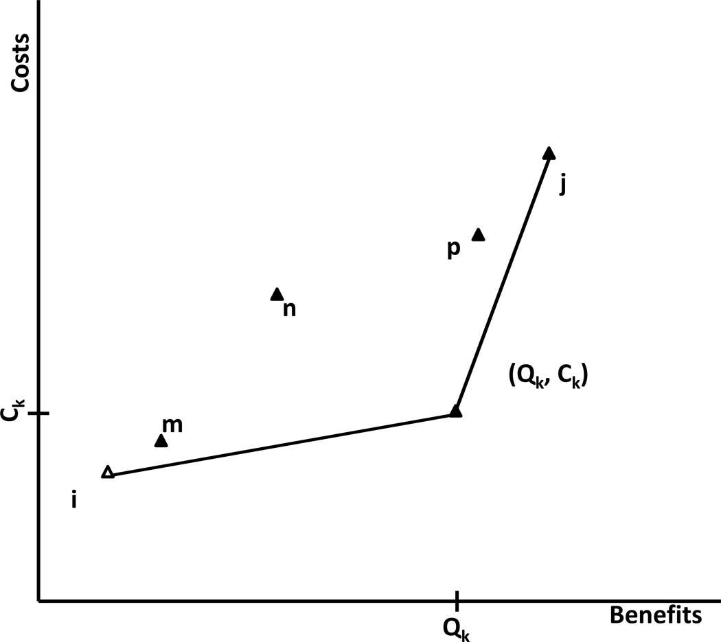
The main result of all cost-effectiveness analyses is the efficient frontier – the set of potentially cost-effective strategies that dominate all other strategies directly or via extended dominance (1). The optimal decision is to choose the strategy with the highest incremental cost-effectiveness ratio (ICER) that falls at or below the threshold willingness-to-pay (WTP) for additional units of benefit, generally expressed as quality adjusted life years (QALYs) in the health policy context (1). We illustrate an example cost-effectiveness plane in Figure 1, for which strategies i, j, and k lie on the efficient frontier and strategies m, n, and p are dominated. While, on expectation, strategies that are off the efficient frontier should not be considered for implementation, they may still be of interest for implementation if, in subgroup analyses, they join the efficient frontier (e.g., the analysis identifies a subpopulation or specific situation in which the strategy would be preferred).
Figure 1. Example Cost-Effectiveness Plane.
Strategies are plotted by cost and benefit (strategy i has cost Ci and benefit Qi) on a cost-effectiveness plane. In this example, strategies i, j, and k lie on the cost-effective frontier (represented by the solid line) and strategy n is strictly dominated (requires higher costs and less benefit than strategy k) while strategy m and p are dominated by extended dominance.
Traditionally, methods for identifying strategies on the efficient frontier can be complicated, requiring an iterative process. The basic algorithm involves the ordering of strategies in terms of ascending cost, eliminating strategies that cost more but provide less benefits than an alternative, computing pairwise ICERs, and then iteratively discarding strategies identified as dominated via extended dominance (i.e., ICER higher than that of the following strategy) until no more strategies can be eliminated. Iteration is required to distinguish those strategies that are dominated via extended dominance since once such a strategy is eliminated, the ICER for the strategy previously compared to it must be recalculated, potentially resulting in the identification of another strategy dominated via extended dominance. This process can be slow in analyses considering large numbers of strategies (2) or in cases when many efficient frontiers must be computed (i.e., for analyses requiring extensive sensitivity analyses). Furthermore, it is more difficult to code de novo and hence potentially more error prone for models implemented in software packages without built-in efficient frontier calculators (e.g., R, Matlab, Excel).
Here, we propose a simple, one-pass alternative to the iterative process of identifying the efficient frontier using the net monetary benefit (NMB), defined as a strategy’s benefits, converted to monetary units for a given WTP, minus its costs. Although the relationship between the NMB and the ICER is well-known (3)(4), the use of this relationship to identify the efficient frontier has not been previously published in reporting deterministic results of a cost-effectiveness analysis.
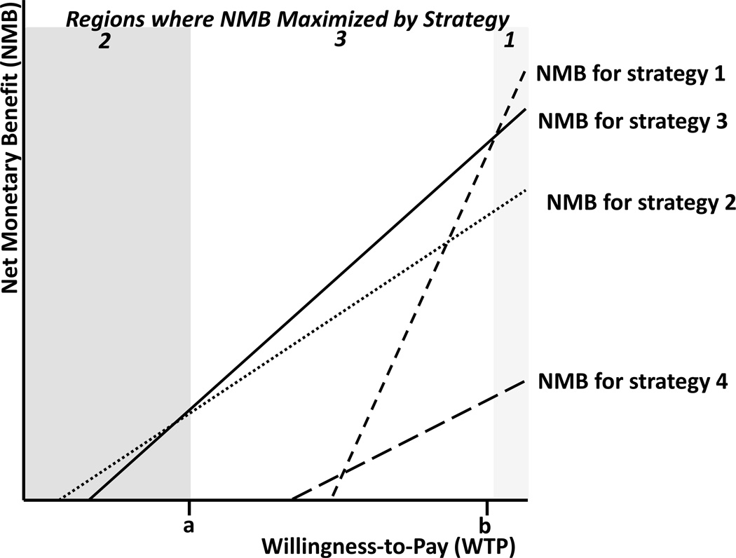
In the proof below, we show that all strategies on the efficient frontier must have the largest NMB for some positive WTP and that strategies that are not on the frontier do not. We illustrate strategies that maximize NMB on a NMB versus WTP plot for a hypothetical study in Figure 2. This means that identifying strategies that maximize the NMB for all WTP levels uniquely identifies the frontier.
Figure 2. Hypothetical NMB versus WTP plot for Four Strategies.
Strategy 2 maximizes NMB for WTP levels between 0 and a, and strategy 3 between a and b, and strategy 1 for WTP levels above b. Strategies 1, 2, and 3 are on the cost-effective frontier, and strategy 4 is dominated. Since only a discrete set of WTP levels are considered with our method, finding the strategy that maximizes NMB at all intersections of NMB lines (equivalent to WTP levels at the pairwise ICERs) will ensure that we capture all and only those strategies on the frontier. (Not testing a WTP level between a and b would result in the omission of strategy 3, for example.) Note that the magnitude of the y-intercepts of each line represent that strategy’s costs, the x-intercept the average effectiveness ratio (cost / benefits), and the slope equal to the benefits.
Our approach requires few lines of code to implement. For example, we use one line and employ Matlab’s “max” function, which gives the value and index of the maximum of each column in amatrix:
[NMB_values, CE_frontier_strategies] = max (health_benefits_vector*WTPvector’ – costs_vector’)
where health_benefits_vector and costs_vector are the total discounted health benefits (measured in QALYs) and costs for each strategy, and WTP_vector is a vector of positive WTP levels; all are column vectors. The WTP vector need only include values relevant to the policymaker (i.e., below a certain threshold). This implementation would calculate the NMB of all the policies at all specified WTP levels, identifying the strategy maximizing NMB at each level. Smaller intervals between the WTP levels reduce the possibility of not capturing a strategy that is only cost-effective over a narrow WTP range; one can ensure that no strategies will be missed if the WTP levels include all pairwise ICERs (see proof).
Proof
We first define what it means to be on the cost-effective frontier (section I), show frontier strategies will maximize the NMB for some positive WTP level (section II), and then show non-frontier strategies will never maximize the NMB for positive WTP levels (section III). Together, section II and III imply that identifying all strategies that maximize the NMB for positive WTP levels will identify only and all frontier strategies.
I. Definition of the Cost-Effective Frontier
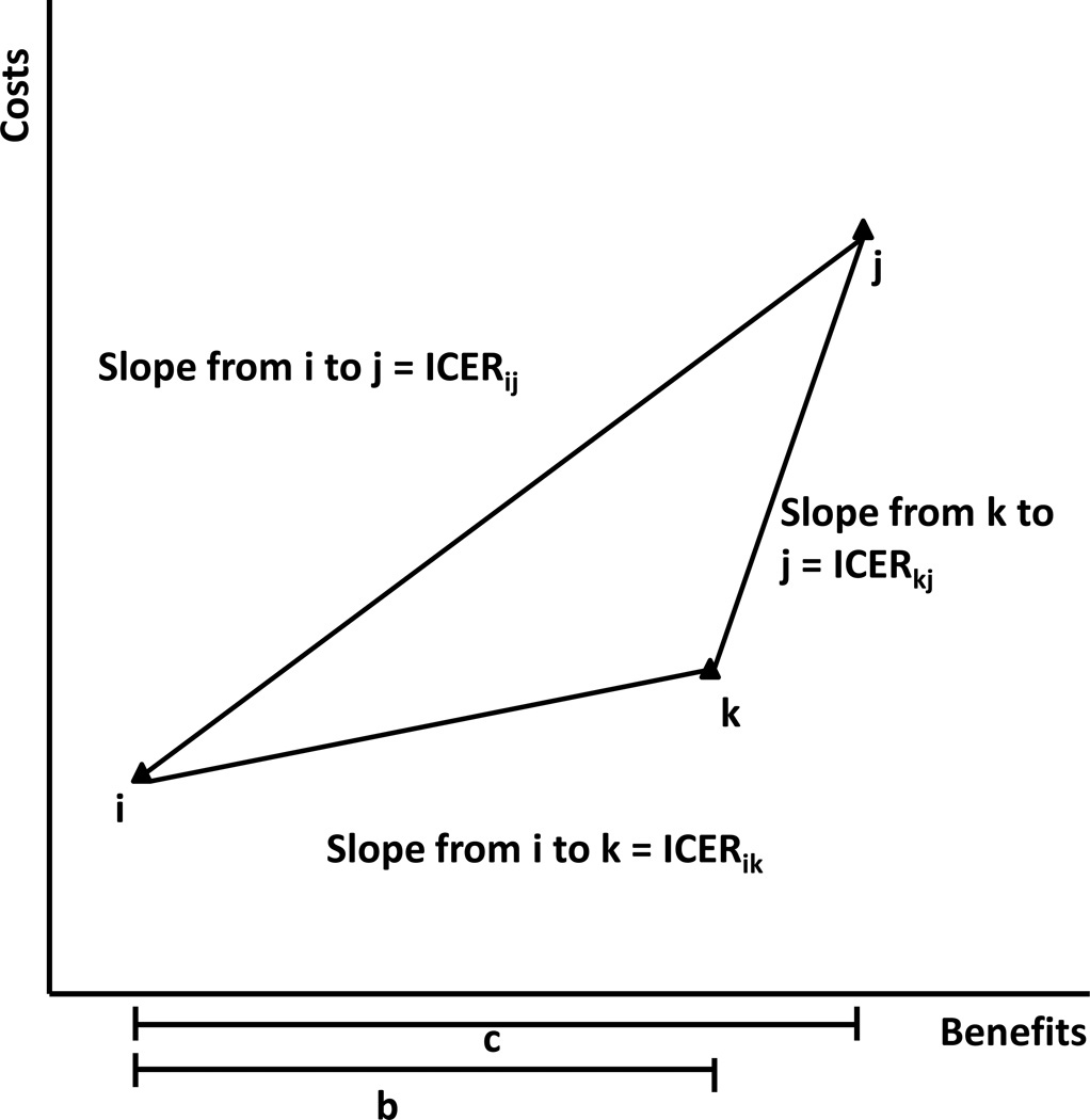
First we define what it means for a strategy to be on the frontier. Let Ci be the total discounted cost and Qi the total discounted health benefits to strategy i. Let strategy k lie between strategy i and j (Figure 3):
| (1) |
| (2) |
Figure 3. Schematic of Strategies as Referred to in the Proof.
Cost-effectiveness plane with strategies i, j, and k. The ICERs are equivalent to the slopes; graphically, it is clear that a value between ICERik and ICERkj must exist (and one such value is ICERij, the slope between i and j). The ratio of distance b to distance c is the proportion a.
For strategy k to be on the efficient frontier in the cost-effectiveness plane, it must lie below the line between strategy i and j:
| (3) |
where a is defined as:
| (4) |
this corresponds to the ratio in Figure 3.
II. Frontier Strategies Will Have the Highest NMB for Some Positive WTP Level
To show that a strategy k on the frontier will have the highest NMB for some positive WTP level, we want to show NMBk ≥ NMB~k, where ~k denotes non-k strategies. Using the definition of NMB with WTP of λ, we require:
| (5) |
| (6) |
and if Qk = Q~k then we want Ck ≤ C~k, which is true if strategy k is on the frontier.
In relation to the strategies i and j introduced in the definition of the frontier, we are therefore trying to find a λ that satisfies:
| (7) |
Or equivalently, ICERki ≤ λ ≤ ICERkj, where ICERki is the incremental cost effective ratio between strategies k and i. I.e., λ must be larger than the slope from i to k and smaller than the slope from k to j on the plot of the strategies on the cost-effectiveness plane. We will show this follows from the definition of being on the frontier. We first rearrange equation 3 and 4:
| (3a) |
| (3b) |
| (4a) |
| (4b) |
then divide (3a) by (4a), which is positive, to find the slope from i to k is smaller than the slope from i to j:
| (8) |
or ICERik ≤ ICERij. Next, dividing (3b) by (4b) and multiplying both sides by negative one to change the sign, we see the slope from k to j is larger than the slope from i to j:
| (9) |
which means ICERjk ≤ ICERij. Using (8) and (9) and setting between i and j we get:
| (10) |
or that λ lies between ICERjk and ICERik. This means that strategy k has the largest NMB for a WTP level equal to the ICER between the strategies to either side of it. Therefore, by considering WTP levels equal to all positive pairwise ICERs -- to ensure that ICERs for all possible i and j have been tested -- along with 0 and the maximum WTP relevant for a given policy analysis, one is guaranteed to identify all desired strategies on the frontier.
III. Non-Frontier Strategies Will Never Have the Highest NMB for Any Positive WTP Level
Next we prove that dominated strategies (both strict and extended dominance) will never have the highest NMB for any positive WTP level to show that we will not mistakenly identify strategies not on the frontier. For a strategy k, sitting between strategy i and j, to not be on the frontier, it must lie above the line between strategies i and j:
| (3’) |
Where a defined as before. Rearranging (3’), we have:
| (3’a) |
| (3’b) |
Equations (4a) and (4b) still hold, implying:
| (8’) |
| (9’) |
| (11) |
| (12) |
Hence no λ exists such that ICERki ≤ λ ≤ ICERkj. Therefore strategies that are strictly dominated or dominated by extended dominance will never have the highest NMB for any positive WTP level.
Until this point, the proof omits the lowest cost and lowest QALY strategy and highest QALY strategy. However, the lowest QALY, lowest cost strategy will be correctly identified as being on the frontier for a WTP level of zero, since maximizing the NMB with WTP of zero is equivalent to finding the lowest cost strategy. This method will therefore also work for a cost-saving strategy, as that might be considered a special case of the lowest cost strategy. The strategy providing the highest number of QALYs is always on the efficient frontier and will be identified for a WTP of infinity, since maximizing the NMB with WTP of infinity is equivalent to finding the highest QALY strategy.
The implication of the proof is that finding all the strategies that maximize NMB at WTP levels defined by all pairwise ICERs identifies all and only those strategies that are on the efficient frontier, and limiting the maximum WTP levels to those below the decision maker’s WTP level identifies the set of strategies on the efficient frontier that provide enough benefit to justify their cost.
The algorithm we developed can be directly used to identify the efficient frontiers for deterministic sensitivity analyses and complements existing approaches for conducting probabilistic analyses (3). By employing concepts common to probabilistic sensitivity analyses in terms of a Net Benefit framework with NMB and WTP, we hope its use will facilitate readers' overall understanding by making the reporting of results from deterministic and probabilistic analyses more consistent. While other algorithms in the same order of operation can be used to identify the cost-effective frontier (since this is equivalent to finding a section of the convex hull on the cost-effectiveness plane, variations on Graham’s algorithm (5), Chan’s algorithm (6), etc. may be used), one benefit of choosing to use this algorithm may be reader understanding and its use of the Net Benefit framework which is commonly used in the medical decision making literature.
To facilitate further evaluation and use, we provide Open Source R and Matlab code that identifies strategies on the frontier for a .csv file of costs and benefits. Users may specify a maximum WTP threshold to exclude strategies that cost more per benefit gained than desired. The code generates a cost-effectiveness plane with efficient strategies highlighted and displays the strategies on the efficient frontier.
Supplementary Material
Acknowledgements
We would like to acknowledge the Hawre Jalal for his discussion on this topic with the authors.
Financial support for this study was provided in part by grants from the National Institute on Aging (K01-AG037593-01A1) and the National Science Foundation Graduate Research Fellowship under Grant No. DGE-114747. The funding agreement ensured the authors’ independence in designing the study, interpreting the data, writing, and publishing the report.
Footnotes
- Example input cost / benefits.csv file, for use with R and Matlab code (CostQalyInputFile_online_supp.csv)
- R code for NMB method of CEAF identification (getFrontier_online_supp.R)
- Matlab code for NMB method of CEAF identification (getFrontier_online_supp.m)
References
- 1.Gold MR, Siegel JE, Russell LB, Weinstein MC. Cost-Effectiveness in Health and Medicine. Oxford University Press; 1996. [Google Scholar]
- 2.Goldhaber-Fiebert JD, Stout NK, Salomon Ja, Kuntz KM, Goldie SJ. Cost-effectiveness of cervical cancer screening with human papillomavirus DNA testing and HPV-16,18 vaccination. [cited 2014 Nov 4];J Natl Cancer Inst [Internet] 2008 Mar 5;100(5):308–320. doi: 10.1093/jnci/djn019. Available from: http://www.pubmedcentral.nih.gov/articlerender.fcgi?artid=3099548&tool=pmcentrez&rendertype=abstract. [DOI] [PMC free article] [PubMed] [Google Scholar]
- 3.Barton GR, Briggs AH, Fenwick EaL. Optimal cost-effectiveness decisions: the role of the cost-effectiveness acceptability curve (CEAC), the cost-effectiveness acceptability frontier (CEAF), and the expected value of perfection information (EVPI) Value Health [Internet] 2008;11(5):886–897. doi: 10.1111/j.1524-4733.2008.00358.x. Available from: http://www.ncbi.nlm.nih.gov/pubmed/18489513. [DOI] [PubMed] [Google Scholar]
- 4.Myriam Hunink MG, Weinstein Milton C, Eve Wittenberg JS, Pliskin Paul P, Glasziou Michael F, Drummond JBW. Decision Making in Health and Medicine. Cambridge University Press; 2014. [Google Scholar]
- 5.Graham R. An efficient algorithm for determining the convex hull of a finite planar set. Inf Process. 1972:132–133. [Google Scholar]
- 6.Chan TM. Optimal output-sensitive convex hull algorithms in two and three dimensions. Discrete Comput Geom [Internet] 1996 Apr;16(4):361–368. Available from: http://link.springer.com/10.1007/BF02712873. [Google Scholar]
Associated Data
This section collects any data citations, data availability statements, or supplementary materials included in this article.


