An Integrated Hierarchical Bayesian Model for Multivariate eQTL Mapping

Abstract

Recently, expression quantitative loci (eQTL) mapping studies, where expression levels of thousands of genes are viewed as quantitative traits, have been used to provide greater insight into the biology of gene regulation. Originally, eQTLs were detected by applying standard QTL detection tools (using a “one gene at-a-time” approach), but this method ignores many possible interactions between genes. Several other methods have proposed to overcome these limitations, but each of them has some specific disadvantages. In this paper, we present an integrated hierarchical Bayesian model that jointly models all genes and SNPs to detect eQTLs. We propose a model (named iBMQ) that is specifically designed to handle a large number G of gene expressions, a large number S of regressors (genetic markers) and a small number n of individuals in what we call a “large G, large S, small n” paradigm. This method incorporates genotypic and gene expression data into a single model while 1) specifically coping with the high dimensionality of eQTL data (large number of genes), 2) borrowing strength from all gene expression data for the mapping procedures, and 3) controlling the number of false positives to a desirable level. To validate our model, we have performed simulation studies and showed that it outperforms other popular methods for eQTL detection, including QTLBIM, R-QTL, remMap and M-SPLS. Finally, we used our model to analyze a real expression dataset obtained in a panel of mice BXD Recombinant Inbred (RI) strains. Analysis of these data with iBMQ revealed the presence of multiple hotspots showing significant enrichment in genes belonging to one or more annotation categories.

1 Introduction

“Complex quantitative traits” are typically defined as characteristics that depend in part on inherited factors, but whose magnitude results from interactions between a great number of genes and environmental factors. Originally, investigators studying such traits focused mostly on physical characteristics and/or physiologic responses, and aimed at locating quantitative trait loci (QTL), i.e. genomic locations that had an influence on the manifested trait. More recently, since expression levels of genes within tissues can themselves be considered as quantitative traits, several studies have identified so-called “expression quantitative trait loci” (eQTL). The identification of eQTLs has provided greater insights into the biology of gene regulation and/or complex traits (Brem et al., 2002, Schadt et al., 2003, Goring et al., 2007). By using DNA microarrays, it has now become feasible to map eQTLs for basically all genes in the genome.

When an eQTL locus corresponds to that of the gene whose transcript abundance is measured, it is identified as a “cis-acting eQTL” (cis-eQTL), meaning that a genetic variation in the neighborhood of the gene is associated with the differential abundance of its transcript. Equally interesting and abundant are the trans-eQTLs that map to locations distant from the gene region. Many studies have reported strong clustering of trans-eQTLs (i.e. multiple genes associated with the same loci) into so-called eQTL hotspots (Zhu et al., 2007, Dixon et al., 2007), which suggests that these genomic regions harbor polymorphisms that shape the dynamic and global nature of transcriptional regulation.

Since eQTL studies differ from standard QTL studies only in the number of phenotypes, it is not surprising that mostly classical QTL methods have been used to identify eQTLs, one gene at a time. However, this “one gene at-a-time” approach ignores the many important combinatorial effects and interactions between genes. Moreover, the multiplicity problem is such that it is not uncommon to have to perform well over a million tests, and univariate methods do not deal appropriately with the problem of multiple testing across markers and genes. Over the years, several strategies have emerged in order to address the multiple issues raised by the high dimensionality of the data at both the trait level (thousands of gene expressions) and the genotype level (thousands of SNPs). For instance, Chun and Keleş¸ (2009) proposed using a Sparse Partial Least Square (SPLS) regression technique to account for the high dimension and co-linearity of the genotype data. Dependence among gene expressions is accounted for by clustering the genes according to their expression profile and then applying the SPLS regression at the cluster level. While very appealing, this method has the drawback of identifying markers associated with a “meta-transcript” instead of individual transcripts. Alternatively, Kendziorski et al. (2006) proposed a Mixture Over Marker (MOM) modeling technique to facilitate information sharing across both markers and transcripts through an empirical Bayes strategy. Although this method identifies transcripts that map to at least one marker, it has the main disadvantage of identifying at most one eQTL per transcript.

Bayesian models have been widely used to solve the extreme multiplicity problem of eQTL studies. By borrowing information across genes and/or markers, they provide efficient ways to overcome the computation burden imposed by the great number of tests required to analyze one gene/one marker at a time. Several approaches based on Sparse Bayesian Regression (SBR) modeling have been developed specifically for QTL studies. For example, the method of Yi et al. (2005), as implemented for eQTL studies in the R-QTLBIM (QTL-Bayesian Interval mapping) package, proceeds by analyzing all SNPs simultaneously but all genes independently. This method was further extended by Banerjee, Yandell and Yi (2008) to handle several traits (genes) simultaneously but is limited in practice to a maximum of five traits, due to computational issues. This approach was generalized to continuous and categorical traits by Xu et al. (2009) and implemented in the BAYES software package. As in the work of Banerjee et al. (2008), this implementation also suffers from the same computational downside and cannot be applied to a large number of traits (i.e. gene expression profiles) as in a typical eQTL studies. Petretto et al. (2010) introduced an efficient evolutionary stochastic search algorithms for variable selection and used it to detect eQTLs across multiple tissues, but their approach models each gene separately and no information is explicitly shared across genes. Recently, Stegle et al. (2010) proposed a Variational Bayes approach (VBQTL) to jointly model the contribution from genotypes as well as known and hidden confounding factors in a unified Bayesian framework. Even though VBQTL models all genes concurrently, the prior probability of association is assumed to be common across all genes and markers, which is unrealistic for such data. In addition, as in the MOM model (Kendziorski et al., 2006), the authors constrain each gene to have at most one relevant SNP regulator for computational reasons.

All the Bayesian models described above assume a common prior distribution for the probability of inclusion of a marker in the sparse regression model, across all genes. As we shall see in the simulations studies, this leads to an over-detection of common eQTLs and thus a high number of false positive hotspots. In this paper, we present an integrated Bayesian hierarchical Model for eQTL mapping (iBMQ) that incorporates genotypic and gene expression data (and possibly thousands of SNPs and genes) into a single model while resolving all the issues mentioned above. Specifically, our model is built around flexible prior distributions and is designed to 1) cope with the high dimensionality of eQTL data (large number of genes), 2) borrow strength from all gene expression data for the mapping procedures, and 3) control the number of false positives to a desirable level. Note that the model developed by Richardson et al. (2010) was developed with similar objectives but for the detection of common eQTLs across tissues. In this slightly different context, the authors had to assume a more restrictive structure on the prior distribution for the probability of inclusion of a marker in the model.

This paper is organized as follows: Section 2 introduces our integrated hierarchical Bayesian Model for Multivariate eQTL Mapping (iBMQ) and specifies the different parameters and their priors. In Section 3, we evaluate our model using a series of simulation studies and compare its performance to several other previously developed methods: 1) R-QTL (Broman et al., 2003), 2) QTLBIM (Yi et al., 2005); 3) M-SPLS (Chun and Keleş¸, 2009); 4) remMap (Peng et al., 2009); and 5) a simplified version of our full iBMQ model that uses a common prior distribution for the probability of inclusion of a marker, i.e. iBMQ with common weight (iBMQ-cw). The latter is in fact similar to the BAYES model (Xu et al., 2009) and VBQTL (Stegle et al., 2010) which both rely on a common prior probability of association. In Section 4, we apply our model to analyze a set of gene expression data obtained in whole eyes from a panel of 68 mice BXD Recombinant Inbred (RI) strains. We conclude in Section 5 with a discussion on possible future improvements of the model.

2 Model

In this section, we present our integrated hierarchical Bayesian Model used to detect eQTLs (iBMQ) and the full conditional distributions used to perform posterior exploration via Markov chain Monte Carlo (MCMC). In the current application and following examples, individuals are in fact RI strains (where particular combinations of parental alleles have been fixed within strains by extensive inbreeding) and genetic markers are Single Nucleotide Polymorphisms (SNPs).

2.1 Model Definition

We model gene expression measurements across individuals as follows,

$$y_{ig}={\mu }_g+\sum _{j=1}^s{x}_{ij}{\gamma }_{jg}{\beta }_{jg}+{\varepsilon }_{ig},$$ (1)

where

• g = 1, …, G denotes a particular gene or a trait, i = 1, …, n denotes a particular strain or individual and j = 1, …, S denotes a particular SNP;

• y_ig is the expression level of gene g for the individual strain i;

• μ_g is the overall mean expression level of gene g (across all strains);

• x_ij represents the genotype at locus j for strain i under an additive, dominant or recessive genetic model;

• β_jg is the effect size of SNP j on gene g. In practice, only a few markers directly affect the phenotype and thus many of the β's should be exactly zero. In order to capture the “sparsity” of the model, we need to incorporate indicator variables, γ_jg, specifying which marker should be included in the model.

• γ_g is a binary inclusion indicator, i.e γ_g = 1 if SNP j is included in the model for gene g and γ_jg = 0 otherwise;

• ε_ig is an error term assumed to be Gaussian with gene specific variance ${\sigma }_g^2$.

In eQTL studies, we have thousands of gene expression profiles as quantitative phenotypes, and analysis of such data typically requires performing univariate QTL analysis for each gene expression profile. The model we propose is motivated by two key factors: 1) most eQTLs affect more than one expression profile, with some affecting many genes; 2) genes in the same pathway are more likely to be under the influence of common regulators (i.e. their expressions are correlated). As a result, there is an opportunity to share information across the hundreds or thousands of gene expression traits in such a way that more informative conclusions can be drawn. This can be done by allowing for a gene/marker-specific probability of QTL, w_jg = ℙ(γ_jg = 1) a priori, and borrow strength across genes to estimate this probability via flexible genome-wide prior distributions; see Figure 2.2 for a graphical representation. Such a hierarchical structure encourages eQTLs to be associated with more than one gene. The rationale is that true eQTLs are probably associated with more than one transcript, while eQTLs that are associated with a single gene are possibly due to noise and should be down weighted, but not necessarily eliminated.

In the proposed model, we assume that the ε_ig's are independent and identically distributed (iid), so that genes are conditionally independent given all model parameters. The gene dependence is introduced via an exchangeable prior on the γ_gj's, thus providing a computationally tractable model with a suitable dependence modeling framework. As we will see in section 3.1, our approach performs well even in the presence of between gene correlations from non-genetic sources.

2.2 Prior Distributions

In the following, we describe the different prior distributions of the model (1). These priors should reflect our a priori knowledge and uncertainty about the model parameters, namely $\theta =({\mu }_g,{\sigma }_g^2,{\gamma }_{jg},{\beta }_{jg},{\omega }_{jg},p_j,a_j,b_j)$. Our priors are defined as follows,

• γ_jg ∼ ℬernoulli(ω_jg), where ℙ(γ_jg = 1) = ω_jg is an unknown parameter that represents the inclusion probability of SNP j in the model for gene g. In order to reduce the false discovery rate, and since only a small numbers of SNPs act as a determinant of a gene expression, we let the inclusion probability parameters ω_jg take the value 0 a priori most of the time. When ω_jg is not 0, it is assumed to come from a Beta distribution ℬeta(a_j, b_j). This can be expressed as a mixture of a Dirac mass at 0 and a Beta distribution with weights p_j and 1 — p_j as follow

  $${\omega }_{jg}~p_j{\delta }_0({\omega }_{jg})+(1-p_j)\mathcal{B}\mathit{\text{eta}}(a_j,b_j)({\omega }_{jg}).$$

  The parameter p_j (the probability that ω_jg is 0) is identical for all genes. This helps in detecting a stronger signal when a SNP is weakly associated to many gene expressions (Lucas et al. (2006)). Furthermore, we use a common conjugate Beta prior for p_j with hyperparameters a₀ and b₀:

  $$p_j~\mathcal{B}\mathit{\text{eta}}(a_0,b_0).$$

  Additionally, a_j and b_j are assumed to follow Exponential distributions with hyperparameters λ_a and λ_b:

  $$a_j~\mathcal{E}\mathit{\text{xp}}({\lambda }_a)\text{and}{b}_j~\mathcal{E}\mathit{\text{xp}}({\lambda }_b).$$

• ${\mu }_g~\mathcal{N}(m_g,{\tau }_g^2)$, where μ_g and τ_g are the empirical mean and variance of gene expression g

• β_jg = 0 if γ_jg = 0 and ${\beta }_{jg}~\mathcal{N}(0,{\nu }_{jg}^2)$ if γ_jg = 1, with ${\nu }_{jg}^2=c{\left(x_j^T{x}_j\right)}^{-1}{\sigma }_g^2$, where c is a scaling factor parameter and ${\left(x_j^T{x}_j\right)}^{-1}={\left(\sum _{i=1}^n{x}_{ij}^2\right)}^{-1}$ mimics the regressor variance, which leads to the well-known g-prior of Zellner (1986). Here we follow the approach of Yi et al. (2005) and consider c to be a constant equal to S the number of SNPs. Bottolo and Richardson (2010) considered an Inverse-Gamma prior $c~\mathcal{I}n\mathcal{G}a(\frac{1}{2},\frac{n}{2})$ based on the Zellner and Siow (1980) prior. Recently Petretto et al. (2010) considered a common c for all genes with the prior of Liang et al. (2008) $c~\frac{1}{1+c}$ in the interval (0, M), where the end point M is M = max(n, S²). The term ${\sigma }_g^2$, the overall variance of ${\nu }_{jg}^2$, ensures that the parameter ${\sigma }_g^2$ is a nuisance parameter in the model and can be integrated out.

• ${\sigma }_g^2~\mathcal{I}n\mathcal{G}a(\frac{1}{2},\frac{1}{2})$ is a vague prior on the error variances.

A graphical representation summarizing our model and its prior specifications is shown in Figure 1. Our model has two clear advantages over alternatives. First, it treats a large number of genes at a time, which effectively facilitates the detection of common eQTLs hotspots that otherwise could not be detected for genes with weak signals if they were analyzed one at a time. The second advantage is that each gene expression/trait has its own inclusion indicator γ_jg at each SNP. In previously published work, the inclusion probability parameters ω_jg were either (i) considered identical for all SNP positions (ω_jg = ω)), with the common ω being considered either given or following a Beta prior distribution (Yandell et al., 2007, Yi and Shriner, 2008); or (ii) supposed identical for all genes but depending on the SNP positions (ω_jg = ω_j), with each ω_j following a Beta prior distribution (Bottolo and Richardson, 2010, Petretto et al., 2010). As we will see in the simulations studies, such assumptions can have a big impact on the performance of the model.

Figure 1.

Graphical representation of the eQTL model. The rectangles represent either fixed hyperparameters or the data, circles represent unknown (and random) quantities. For each gene, the gene expression phenotype y_g is expressed as a linear model $y_{ig}={\mu }_g+\sum _{j=1}^s{x}_{ij}{\gamma }_{jg}{\beta }_{jg}+{\varepsilon }_{ig}$ The gene/marker specific regression coefficient β_jg is assumed to be normally distributed with distribution ${\beta }_{jg}~\mathcal{N}(0,c{\gamma }_{jg}{(x_j^T{x}_j)}^{-1}{\sigma }_g^2)$. The prior for μ_g is, $\mathcal{N}(m_g,s_g^2)$, and the prior for σ² is π(σ²) ∝ 1/σ². The prior distribution for γ_jg is assumed to be Bernoulli with parameter w_jg. The w_jg's are given ω_jg ∼ p_jδ₀(ω_jg) + (1 – p_j)ℬeta(a_j, b_j)(ω_jg). Additionally, a_j and b_j are assumed to follow Exponential distributions with hyperparameters λ_a and λ_b and p_j ∼ ℬeta(a₀,b₀).

2.3 Parameter Estimation

Realizations were generated from the posterior distribution via MCMC algorithms (Gelfand and Smith, 1990). All updates were done via Gibbs sampling except for a_j and b_j for which no closed form full conditionals are available, and were thus updated via adaptive rejection sampling (Gilks and Wild, 1992). All full conditionals are given in Appendix A. We used the method of Raftery and Lewis (Raftery et al., 1992, 1996) to determine the number of iterations, based on a short pilot run of the sampler. For each dataset presented here, this suggested that a sample of no more than about 1,000,000 iterations with 50,000 burn-in iterations was sufficient to estimate standard posterior quantities. Guided by this, and leaving some margin, we used 2,000,000 iterations after 50,000 burn-ins for each dataset explored here. Results from the diagnostics test and trace plots are presented in Appendix 5. Finally, our model depends on four hyperparameters a₀, b₀, λ_a and λ_b that need to be fixed in advance. We can choose these values a priori using the expected number of e-QTLs (n_γ) and its dispersion (n_γ), as detailed in Appendix B. Using this approach we have chosen a₀ = λ_a = 10 and λ_b = b₀ =.1, which favors models with fewer eQTLs.

2.4 Inference and Detection of eQTLs

Our ultimate goal is to identify gene/SNP associations, and this can be done using parameter estimates from our model. An eQTL for gene g at SNP j is declared significant if its corresponding marginal posterior probability of association (PPA), i.e. Pr(γ_jg = 1|y), is greater than a given threshold. In the context of multiple testing and discoveries, a popular approach is to use a common threshold leading to a desired false discovery rate (FDR). In the Bayesian paradigm, derivation of the PPA threshold is trivial and can be calculated using a direct posterior probability calculation as described in Newton et al. (2004).

3 Simulation Study

We performed two sets of simulation studies: a validation study and a comparison study. The goal of the validation study was to investigate the effects of different factors such as the correlation between SNPs/genes, the effect size and the spatial structure of the true eQTLs with regards to our model's performance. In the comparison study, we compared the performance of our proposed model with other standard methods.

3.1 Validation Study

For the first experimental set, we used n = 100 individuals, G = 40 genes, S = 1000 SNPs and ${\sigma }_g^2=0.1$; the latter two values being taken from the experimental data (section 4). We also considered two types of correlation structures between SNPs and genes. First, SNPs were considered as either independent or dependent. In the latter case, SNPs were divided into 100 blocks of 10 SNPs each. We assumed that blocks were independent and imposed a correlation ρ_x = 0.4 among the SNPs within each block. Second, genes were also considered as either independent or dependent (i.e. correlated, meaning that they show some level of co-expression due to non-genetic causes). In the latter case, genes were divided into 4 independent blocks of 10 consecutive genes each and we chose a correlation ρ_ε = 0.5 within each block. In addition, we simulated two different scenarios for eQTLs positions within gene blocks. These scenarios are illustrated in Figure 2 (a-b) and mimic situations where correlations among genes are due to either genetic causes (when they share the same SNP) or non-genetics causes (when genes belong to the same block of genes). In the first scenario, 7 genes share a common eQTL and 8 genes share a common eQTL at another SNP, with 4 genes having both eQTLs in common. In the second scenario, each of the total 40 genes have either 0, 1, 2 or 3 eQTLs. When a gene had more than 1 eQTL, the eQTLs were selected on different SNP blocks. For all scenarios, eQTLs were simulated using two different values of the regression coefficients: β* = 0.5 and β* = 0.2. These values, based on the values estimated on the experimental data used in section 4, allowed us to compare the performance of the model in situations where the magnitude of the effect due to genetic causes varied from small to large. Altogether, the various situations described above amounted to 16 different combinations. In each case, eQTLs were called using an FDR level of 10%.

Figure 2.

Graphical illustration of the scenarios used for the simulation study. Rows represent genes (divided into 4 blocks of 10 correlated genes each), columns represent SNPs and red dots correspond to simulated eQTLs. In the third scenario, the size of red dots is proportional to the strength of the eQTL association and corresponds to β* = 1, β* = 0.5 and β* = 0.2.

Table 1 shows the sensitivity, specificity, positive predictive value, and negative predictive value obtained with our model across the different simulation settings we described. These values were computed based on the total number of false positive and false negative across all genes and SNPs (this means that a false positive SNP on 2 different genes would be counted twice).Table 1 also shows the effects of different parameters on the detection of eQTLs and the capability of our model to perform even in difficult situations. In particular, we observed that correlation between SNPs had a very small impact on eQTL detection, and that the model had difficulty in detecting eQTLs with small effect sizes (β* = 0.2). Further investigation showed that this was true except in cases where many genes with weak association values all share one identical SNP (results not shown).

Table 1.

Sensitivity, specificity, positive predictive value (PPV) and negative predictive value (NPV) obtained by our model. The value on the first line is for the first eQTL scenario and the value on the second line is for second eQTL scenario. The standard deviation over the 50 replications are presented in parentheses. We used a FDR threshold value of 10% for calling eQTLs.

	gene	SNP	Sens.	Spec.	PPV	NPV
β* = 0.5	indep.	indep.	0.848(0.225)	1(0)	0.17(0.037)	1(0)
			0(0)	0.999(0)	1(0.002)	0.999(0)
		dep.	0.86(0.222)	1(0)	0.182(0.053)	1(0)
			0.001(0.03)	0.999(0)	0.999(0.003)	0.999(0)
	dep.	indep.	0.787(0.227)	1(0)	0.173(0.043)	1(0)
			0(0)	0.99(0)	1(0.002)	0.999(0)
		dep.	0.891(0.198)	1(0)	0.17(0.045)	1(0)
			0(0)	0.99(0)	1(0)	0.999(0)
gene	SNP	Sens.	Spec.	PPV	NPV
β* = 0.2	indep.	indep.	0.12 (0.126)	1(0)	0.226(0.403)	1(0)
			0(0)	1(0)	1(0)	0.99(0)
		dep.	0.104 (0.0114)	1 (0)	0.311 (0.458)	1(0)
			0 (0)	1(0)	0.01(0.02)	0.99(0)
	dep.	indep.	0.16(0.202)	1(0)	0.303(0.4.47)	1(0)
			0(0)	1(0)	1(0)	0.99(0)
		dep.	0.108(0.28)	1(0)	0.28(0.443)	1(0)
			0(0)	1(0)	1(0)	0.99(0)

3.2 Comparison Study

The second set of experiments was based on settings bearing more resemblance to real datasets. The simulated-eQTL distribution is illustrated in Figure 2 (c): 10 genes have three eQTLs each (one cis-eQTL, one trans-eQTL and one hotspot common to all 10 genes), one gene has one eQTL, and three genes have two eQTLs each. The regression coefficients were selected (randomly but once for all replications) among the values 0.2, 0.5 and 1. The total number of genes (40) and SNPs (1000) and error variance ${\sigma }_{\varepsilon }^2=0.1$ were set as in the previous simulation study. The first settings were performed with n = 75 and the other settings were performed in order to show the effect of the population size n on the identification and magnitude of detected eQTLs: we repeated the previous settings with n = 50 and n = 25 individuals all other parameters remaining the same. For each setting, we used 50 replications and results were averaged post-processing over the 50 replications.

In this section, we compare the performance of iBMQ to that of QTLBIM (Yi et al., 2005), M-SPLS (Chun and Keleş¸, 2009), R-QTL (Broman et al., 2003), remMAP (Peng et al., 2009), and iBMQ with common inclusion weight (iBMQ-cw). The utility of each tested model and settings used for each are as outlined as follows,

• QTLBIM. This Bayesian model is similar to our implementation but was originally designed for classical QTL studies, and thus enables the analysis of only one gene at a time. When applying QTLBIM for comparison, we simply ran it G = 40 times, one gene at time. We disabled the options “genome update” and “epistasis effect” and we used the same number of iterations, burn-in and recording sweeps as in the other methods we compare. We set the mean prior number of eQTLs to 3 and the maximum number of eQTLs to 8. We noticed that QTLBIM has a tendency to detect accessory signals on SNPs that surround the SNP associated with the main signal. When computing the results, we aggregated main and accessory SNPs as only one signal.

• M-SPLS. In this approach, a first step consisted in clustering genes into groups on the basis of their expression similarity. We have used the R package Mclust (Yeung et al., 2001) for gene clustering and did a sparse partial least-squares (SPLS) regression on the optimal number of clusters. SPLS does not output posterior probabilities, but calculates bootstrapped confidence intervals of SPLS coefficients with default parameters for each simulation.

• iBMQ-cw. This simplified version of iBMQ was used (with the same parameters as iBMQ except for w, which is common to all genes/SNPs) and can be representative of other models that make the same assumption, e.g. BAYES (Xu et al., 2009) and VBQTL Stegle et al. (2010).

• R-QTL. This non-Bayesian tool was designed initially for classical phenotypic QTL studies. It corresponds to the simplest method, and is still used in the vast majority of real data studies. When applying R-QTL for comparisons, we simply ran it G = 40 times, one gene at time. The interval mapping option was disabled. We have performed a permutation test to get a genome-wide LOD significance threshold per gene.

• remMap. We have also performed a comparison using the remMap method, which implements a penalized regression approach, and used the BIC procedure to select tuning parameters.

In each case, eQTLs were called by controlling the false discovery rate (FDR) at 10% except for remMap, which only performs variable selection and does not compute uncertainty measures (e.g. p-values or posterior probabilities).

The results of the simulations are shown in Figure 3 and Figure 4. Figure 3 compares the ROC curves of iBMQ to those obtained with the other approaches for the different scenarios. Figure 4 shows the PPA plot (for iBMQ, iBMQ-cw and QTLBIM) or the frequency of associations (for M-SPLS and R-QTL) for 20 genes (10 of which sharing the common eQTL “hotspot”) for the setting with 25 individuals. This figure shows the gain of power of iBMQ compared to QTLBIM and M-SPLS while showing the gain in flexibility compared to iBMQ-cw. Regarding the population size, we observed that all models lose power when the number of individuals decreases. However, even when simulating a population as small as 25 individuals, iBMQ still detected most eQTLs with β* coefficient higher than 0.2. Figure 4 allows us to understand the behavior of the model in a more visual fashion. A comparison of iBMQ to QTLBIM and R-QTL shows that iBMQ is better at detecting eQTLs within hotspots. A comparison with iBMQ-cw shows that both models are good at detecting eQTLs within hotspots, but that iBMQ-cw generates noisy signals outside of the hotspots due to the common weight, which has a tendency to include non relevant SNPs into the model. In addition, M-SPLS fails to detect many eQTLs outside of the hotspots, possibly because of the initial clustering, thus showing to what extent the latter can influence the results. iBMQ gains power by sharing information across genes but the model is flexible enough not to create background noise. Overall, the analyses showed that iBMQ increased the power of detecting eQTL hotspots while keeping a low false positive rate, particularly in cases with a small number of individuals. The detection of eQTL hotspots represents an important gain of the multivariate model versus univariate ones in situations where many genes display weak associations with one common shared SNP. Note that for simulations with the present parameters (n <= 75) remMap did not detect any eQTLs.

Figure 3.

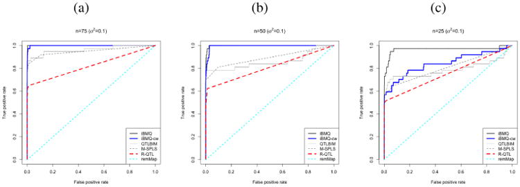
The Receiver Operating Characteristic (ROC) curves of iBMQ, iBMQ-cw, QTLBIM, M-SPLS, R-QTL and remMap for the three different simulation scenarios. a) The ROC curves represent results of the n = 75, b) the curves present the results of the n = 50, c) the curves present the results of the simulation with n = 25. Note that remMap does not detect any eQTLs, hence the line y = x.

Figure 4.

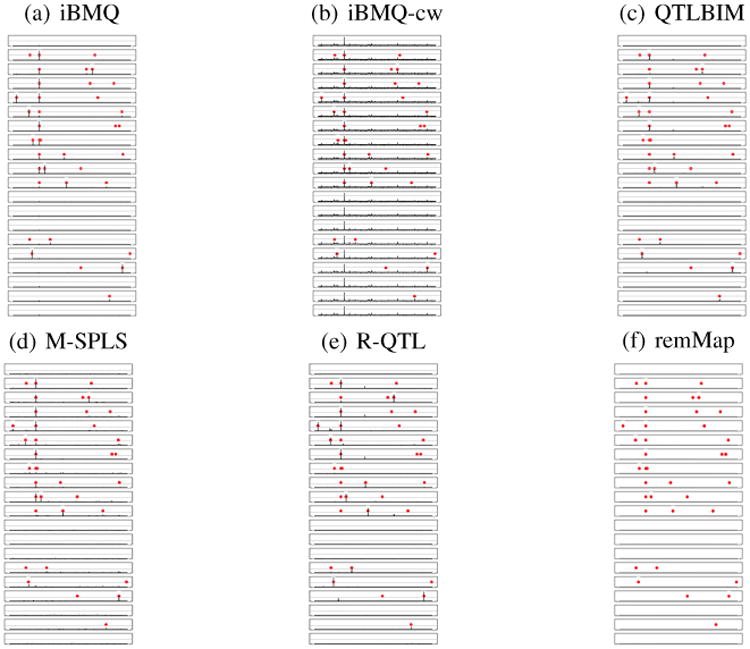
Association plots of 20 genes (simulation with 25 individuals): 10 genes share a common eQTL “hotspot”. The grey horizontal lines correspond to the PPA cutoff used for eQTL detection (corresponding to a False Discovery Rate of 10%), and the red dots represent true eQTLs. a) Posterior Probability plots obtained with iBMQ: the method detects 8/10 genes in the hotspot; b) Posterior Probability plots obtained with iBMQ-cw: the method detects all 10 genes in the hotspot. Although all 10 genes in the hotspot are detected, all other genes (which should not be detected), also display a significant PPA for that SNP; c) Posterior Probability plots obtained with QTLBIM: the method detect only 4/10 genes in the hotspot; d) Frequency of detection of associations with M-SPLS over 50 simulations: the methods detects 7/10 genes in the hotspot; e) Frequency of detection of associations with R-QTL over 50 simulations: the method detects 4/10 genes in the hotspot. f) Frequency of detection of associations with remMap over 50 simulations: this methods did not detect any eQTLs under the present parameters.

4 Application to Data from Mouse RI Strains

In this section, we have applied our model to the whole eye tissue data generated by Williams and Lu, and available from the Gene Network Website (genenetwork.com). This dataset consists of the mRNA profiles of whole eye tissue from n = 68 BXD RI mouse strains, as measured using Affymetrix M430 2.0 microarrays (Geisert et et al., 2009). To ease calculation and facilitate comparison with other methods we set G = 1000 corresponding to the probes showing the highest variation in expression level, while all 1700 markers (SNPs) were used. Such preselection of high variance genes is often done in eQTL studies to facilitate computation and increase power (Richardson et al., 2010).

After applying the direct posterior probability approach and determining a cutoff corresponding to an FDR of 10% (corresponding PPA= 0.74), iBMQ detected a total of 759 significant eQTLs, in comparison to 182 eQTLs detected by QTLBIM (FDR of 10%, PPA≥ 0.44), 1400 eQTLs detected with M-SPLS (FDR of 10%) and 5727 eQTLs detected with R-QTL (FDR of 10%). The remMap method detected a total of 1365 eQTLs (when considering all results different from zero as eQTLs). The overlap eQTLs detected by the different methods is presented by in the Table 2. The genome-wide distribution of eQTLs found by all 3 methods provides further information about the performance characteristics of each model (see Figure 5). Almost all eQTLs detected by QTLBIM were in fact cis-eQTLs (as represented on the diagonal of Figure 5b). Our iBMQ method detected (in addition to the cis-eQTLs represented on the diagonal) several “hotspots” of trans-eQTLs (represented by the dots aligning along vertical lines in Figure 5a). Finally, M-SPLS did not detect any cis-eQTL, but identified several large groups of trans-eQTLs (Figure 5c). Altogether, the number of hotspots containing more than 30 probes amounted to 5 for iBMQ, 3 for remMap, and 16 for M-SPLS. No hotspots were detected by R-QTL and QTLBIM.

Table 2.

Overlap of eQTL detection between different methods. All numbers originate from tests perform with 5 different methods on the real data set. The total number of eQTLs detected by each method is presented between parentheses. Each column contain the number of eQTLs detected in common for a given methods.

	iBMQ	QTLBIM	M-SPLS	R-QTL remMap
iBMQ (759)
QTLBIM (182)	66
M-SPLS (1400)	33	0
R-QTL (5727)	139	113	2
remMap (1365)	0	0	0	11

Figure 5.

Genome-wide distribution of eQTLs found by a) iBMQ, b) QTLBIM, c) M-SPLS, d) R-QTL and e) remMap for the 1000 probes showing most variance of expression in the whole eye tissue from 68 BXD mouse recombinant inbred strains. The x-axis gives the position of each eQTL along the genome; the y-axis gives the position of the probe set target itself. The grey lines mark chromosome boundaries. Cis-QTLs form a diagonal line. Vertical bands represent groups of transcripts linked to a single trans-eQTL. iBMQ detects hotspots of trans-eQTLs (on chromosomes 2,4,8,10 and 12) that are not detected by QTLBIM. No cis-eQTL are detected by M-SPLS. d) R-QTL detect cis-eQTL but virtually no trans-eQTLs. e) No cis-eQTL are detected by remMap and the trans-eQTL hotspot do not overlap those detected by iBQM nor M-SPLS.

To verify whether the hotspots detected by iBMQ (and not by the other 4 methods) showed biologic relevance and coherence, we tested whether corresponding groups of trans-eQTLs showed enrichment in genes belonging to categories within Gene Ontology, using the DAVID Bioinformatics Resources analysis of Huang et al. (2009) (Table 3-4). Five hotspots comprising more than 30 genes were found on 5 different chromosomes. Interestingly, each hotspot showed enrichment for genes related to a GO term dealing with characteristics and properties of epithelial cells (Table 3). One hotspot was enriched in genes corresponding to the “Epithelial cell differentiation” GO term. Other genes belonged to 2 other related GO term categories, and comprised almost exclusively gene from the claudin and keratin families, both of which play essential roles in the maintenance of epithelial cell functions. All 3 GO terms thus dealt with the characteristic and properties of epithelial cells, which may be in keeping with the fact that the majority of cells within whole eye tissue (including the eye bulb, the conjunctiva and the cornea) are epithelial in nature. It is interesting to note that some genes were specific to each hotspot while others were found repeatedly in several hotspots on different chromosomes (Table 4). Although the 3 GO categories corresponding to the hotspots were also detected when testing for enrichment in the whole set of genes corresponding to the 1000 probes showing highest level of variance in expression, these 3 GO categories were underrepresented: only 2 out of the 3 above GO categories were represented among the 50 most significant GO categories in the original dataset, and they ranked only fourteenth and twenty-third in terms of significance of enrichment. In particular, categories corresponding to photoreceptor functions showed most significant enrichments and represented the majority of enriched categories. Thus, the enrichment of the functions related to epithelial cell in the hotspot analysis is not likely to be a mere reflection of category enrichment in the original dataset. Of note, the selection of only a fraction of genes in the dataset was performed to facilitate comparisons across methods. A comprehensive analysis of all eQTL hotspots would require longer calculations using all gene expression data, but could possibly detect other hotspots in addition to the ones reported here, including hotspots of genes related to other functions (such as for instance retinal genes).

Table 3.

Number of probes in each hotspot where iBMQ identified more than 30 trans-eQTL genes, along with information about the GO annotation term for which genes in the hotspot show enrichment for and enrichment statistics. The asterisk (*) identifies annotation terms dealing with characteristics and properties of epithelial cells. The “percent” column represents the percentage of genes found with the GO terms with respect to the total number of genes in the hotspot.

SNP	No of probes	Annotation	Go Term	Percent	P-value
rs4223510 (chr 2)	132	Epithelial cell diff.*	0030855	11.4	4.1e10
rs3687764 (chr 4)	90	Structural molecule act.*	0005198	13.9	0.00012
gnf06.037.785 (chr 8)	32	Structural molecule act.*	0005198	21.7	0.0017
rs13480522 (chr 10)	142	Structural molecule act.*	0005198	11.8	0.000079
rs6376011(chr 12)	33	Intermediate filament*	0005882	16.7	0.00053

Table 4.

For each hotspot from Table 3, there was significant enrichment for genes belonging to Gene Ontology (GO) categories. All corresponding genes are listed under the GO term they belong to. Genes present on hotspot on different chromosomes are formatted in bold.

Chr 2	Chr 4	Chr 8	Chr 10	Chr 12
GO:0030855	GO:0005198	GO:0005198	GO:0005198	GO:0005882
E74-like factor 3	claudin 4	claudin 23	claudin 23	keratin 1
ets homologous factor	claudin 7	claudin 7	claudin 4	keratin 10
keratin 14	keratin 13	keratin 14	claudin7	keratin 13
keratin 17	keratin 14	keratin 16	collagen type III	keratin 14
keratin 4	keratin 19	keratin 4	keratin 13
keratin 6A	keratin 4		keratin 14
patched homolog 1	keratin 6A		keratin 15
stratifin	keratin 7		keratin 19
small proline-rich protein 1A			keratin 4
trans. related protein 63			keratin 6A keratin 7

5 Discussion

In this paper, we introduced an integrated Bayesian model for eQTL mapping, iBMQ, that can handle simultaneously thousands of genes and thousands of SNPs. Our methodology is designed to deal with any Bayesian regression problem even when data are available for a limited number of individuals and when the number of measurements (gene expression and/or traits) per individual and the number of regressors (SNPs) are large. The main contribution of our model is that the association binary indicator γ_jg (between SNP j and gene g) and the corresponding association probability ω_jg of a SNP is specific for each gene and each SNP. In previous studies the association indicators γ_j were common for all genes, and the probability of association was considered as either constant ω over genes and SNPs, or dependent only on SNPs and identical for all genes ω_j. We believe that this is one of the strengths of our modelization as it helps in the detection of hotspots, as supported by the results of the simulation studies.

Our model could still be further refined when non-genetic correlations among gene expressions are large compared to the level of genetic correlations. One theoretically “obvious” solution to this issue consists in relaxing the hypothesis of the independence of errors assumed in model (1). In practice, however, this is an unfeasible challenge in terms of tractability, conjugacy and computability In fact, if genes are no longer presumed independent, the variances ${\sigma }_g^2$, g = 1,…, G need to be replaced by a variance-covariance matrix Σ. To keep the conjugacy of the priors and hence an analytical integration of the posterior distribution for Σ, we have to select an Inverse Wishart (as a generalization to the Inverse Gamma) distribution for Σ as described in Bottolo and Richardson (2010) and Petretto et al. (2010), among others. Although this works well in models where the association indicator γ_jg is common to all genes, it is not feasible in the model we propose, as it will lead to a loss of the conjugacy property and represent a heavy computational issue. As an alternative, we shall try in future work to incorporate correlations among genes by considering blocks of genes within the model, as this might improve the detection of weak associations.

Other future work will also consider the issues of correlation among SNPs due to linkage disequilibrium. It is unrealistic to totally neglect these issues mainly in highly dense genetic maps: as genetic maps become denser, the correlations between nearby SNPs become higher. A starting point may be the the concept of (left and right) flanking SNPs (Yi et al., 2005), with the construction of SNP blocks being potentially useful to convert the concept of neighbours in term of probabilities.

In this article, we have compared our model with five alternatives, but there are other methods for analyzing eQTL data. While additional methods are available (Stegle et al., 2010), we chose these five because they are either obvious baseline methods, widely used or have already been compared to other methods (Chun and Keleş, 2009). Note that the recent work on Bayesian models for sparse regression analysis of high dimensional data in Richardson et al. (2010) also provides a good alternative to our model, as a multiplicative model for the probability structure of the association binary indicator γ_jg is presented.

While our model requires more computing than some other methods because it integrates all genes and SNPs jointly via MCMC (Appendix C), we believe that the improved results are worth the additional computing time. In addition, our current C implementation makes use of the openMP API (Dagum and Menon, 1998) and automatically parallelizes calculations over genes, which can dramatically improve computational time for large datasets. The current implementation of iBMQ in R and C is available from GitHub: https://github.com/raphg/iBMQ. An R package is currently under preparation to be made available via the Bioconductor project (Gentleman et al., 2004).

Figure 6.

Trace plot of parameters a_j, b_j, μ_g and σ_g for three gene/SNP combination with low, medium and high PPA. These plots are based on 2,000,000 iterations after 40,000 burn-in.

Appendix

Appendix A: Full conditional posterior distributions

The set of parameters of the model is $\theta =({\mu }_g,{\sigma }_g^2,{\gamma }_{jg},{\beta }_{jg},{\omega }_{jg},p_j,a_j,b_j)$. The posterior distribution of the parameter set θ is given by the product of the prior distributions π(θ) with the likelihood L(y|x, θ), that is

$$\pi (\theta |y,x)\propto \pi (\theta )L(y|x,\theta )(2)$$ (2)

Where

$$L(y|x,\theta )\propto \prod _{g=1}^G\prod _{i=1}^n\frac{1}{{\sigma }_g}exp(-\frac{1}{2{\sigma }_g^2}{(y_{ig}-{\mu }_g-\sum _{j=1}^S{x}_{ij}{\gamma }_{jg}{\beta }_{ig})}^2).$$

For a specific parameter θ_k, the full conditional π(θ_k| …) is obtained by conditioning the posterior π(θ|y, x) in (2) on the remaining parameters.

• The full conditional of μ_g is ${\mu }_g\sim \mathcal{N}(m_g^{\prime },{\tau }_g^{\prime 2})$, where $m_g^{\prime }$ and ${\tau }_g^{\prime 2}$ are obtained by updating the prior parameters m_g and τ_g as follows:

  $$m_g^{\prime }=\frac{\sum _{i=1}^n(y_{ig}-\sum _{j=1}^S{x}_{ij}{\gamma }_{jg}{\beta }_{jg})/{\sigma }_g^2+m_g/s_g^2}{n/{\sigma }_g^2+1/s_g^2}\text{and}{\tau }_g^{\prime 2}={(n/{\sigma }_g^2+1/s_g^2)}^{-1}.$$

• The full conditional of ${\sigma }_g^2$ is ${\sigma }_g^2~\mathcal{I}n\mathcal{G}a(d_g^{\prime },e_g^{\prime })$, an Inverse Gamma distribution with parameters $d_g^{\prime }$ and $e_g^{\prime }$ where $d_g^{\prime }=\frac{1}{2}(n+1+S_g)$ and

  $$e_g^{\prime }=\frac{1}{2}\sum _{i=1}^n{(y_{ig}-{\mu }_g-\sum _{j=1}^S{x}_{ij}{\gamma }_{jg}{\beta }_{jg})}^2+\frac{1}{2c}\sum _{j=1}^S\left({\gamma }_{jg}{\beta }_{jg}^2\sum _{i=1}^n{x}_{ij}^2\right).$$

• The parameters γ_jg and β_jg require special attention. These two parameters are updated simultaneously using their joint full conditional π(γ_jg, β_jg|…). We first sample γ_jg from the marginal posterior π(γ_jg|…) obtained by integrating out β_jg in π(γ_jg,β_jg|…) and then β_jg is simulated from the conditional distribution π(β_jg|γ_jg, …). The joint full conditional π(γ_jg,β_jg|…) is given by

  $$\pi ({\gamma }_{ig},{\beta }_{jg}|\dots )\propto L({\gamma }_{jg},{\beta }_{jg}|\dots )\pi ({\gamma }_{jg}|{\omega }_j)\pi ({\beta }_{jg}|{\gamma }_{jg}),$$ (3)

  where L(γ_jg, β_jg |…) is the part of the likelihood containing γ_jg and β_jg (i.e. the contribution of gene expression g) and is given by

  $$L({\gamma }_{jg},{\beta }_{jg}|\dots )\propto \prod _{i=1}^n\frac{1}{{\sigma }_g}exp(-\frac{1}{2{\sigma }_g^2}{(y_{ig}-{\mu }_g-\sum _{j\prime =1}^S{x}_{ij\prime }{\gamma }_{jg\prime }{\beta }_{jg\prime })}^2).$$

  Furthermore, in equation (3), $\pi ({\gamma }_{jg}|{\omega }_{jg})={\omega }_{jg}^{{\gamma }_{jg}}{(1-{\omega }_{jg})}^{1-{\gamma }_{jg}}$ is the Bernoulli prior of γ_jg and π(β_jg|γ_jg) is the prior distribution of β_jg conditional on γ_jg such that:

  $$\pi ({\beta }_{jg}|{\gamma }_{jg})={\delta }_0({\beta }_{jg}){\mathbb{I}}_{({\gamma }_{jg}=0)}+\mathcal{N}(0,v_{jg}^2)({\beta }_{jg}){\mathbb{I}}_{({\gamma }_{jg}=1)}.$$

  In order to sample γ_jg from π(γ_jg|…), we integrate out β_jg and we let

  $$p_0=\int L({\gamma }_{jg}=0,{\beta }_{jg}|\dots )\pi ({\beta }_{jg}|{\gamma }_{jg}=0)d{\beta }_{jg}=L({\gamma }_{jg}=0,{\beta }_{jg}=0|\dots ),$$

  $$p_1=\int L({\gamma }_{jg}=1,{\beta }_{jg}|\dots )\pi ({\beta }_{jg}{\gamma }_{jg}=1)d{\beta }_{jg}.$$

  It follows that π(γ_jg = 0|…) ∝ (1 – ω_jg)p₀ and π(γ_jg = 1|…) ∝ ω_jgp₁. Further computation leads to p₁ = Cp₀, where the quantity C is equal to

  $$\mathrm{C}=1\frac{}{{(1+c)}^{1/2}exp\left(\frac{1}{2}\frac{c}{(1+c){\sigma }_g^2\sum _{i=1}^n{x}_{ij}^2}{[{\sum }_{i=1}^n{x}_{ij}(y_{ig}-{\mu }_g-{\sum }_{j\prime \ne j}{x}_{ij\prime }{\gamma }_{jg\prime }{\beta }_{jg\prime })]}^2\right).}$$

  Finally, the parameter γ_jg is sampled from $\pi ({\gamma }_{jg}=0|\dots )=\frac{1-{\omega }_{jg}}{C{\omega }_{jg}+(1-{\omega }_{jg})}$ and $\pi ({\gamma }_{jg}=1|\dots )=\frac{C{\omega }_{jg}}{C{\omega }_{jg}+(1-{\omega }_{jg})}.$

  As we mentioned earlier, the parameter β_jg is sampled from the conditional posterior distribution π(β_jg|γ_jg). Precisely, β_jg = 0 if γ_jg is sampled as 0 and β_jg is generated from a $\mathcal{N}(m_{jg}^{\prime },v_{jg}^{\prime 2})$ if γ_jg is sampled as 1. The quantities $m_{jg}^{\prime }$ and $v_{jg}^{\prime 2}$ are given by

  $$m_{jg}^{\prime }=\frac{c}{(1+c)\sum _{i=1}^n{x}_{ij}^2}\sum _{i=1}^n{x}_{ij}(y_{ig}-{\mu }_g-\sum _{j\prime \ne j}{x}_{ij\prime }{\gamma }_{ij\prime }{\beta }_{ij\prime })$$

  $$v_{jg}^{\prime 2}=\frac{c{\sigma }_g^2}{(1+c)\sum _{i=1}^n{x}_{ij}^2}.$$

• The full conditional of ω_jg is ${\omega }_{jg}~r{\delta }_0({\omega }_{jg})+(1-r)\mathcal{B}\mathit{\text{eta}}(a_j^{\prime },b_j^{\prime })({\omega }_{jg})$, which is a mixture of a Dirac mass in 0 and a Beta distribution with parameters $a_j^{\prime }=a_j+{\gamma }_{jg}$ and $b_j^{\prime }=b_j+1-{\gamma }_{jg}$ and with respective weights r and 1 – r, where r is given by

  $$r=\frac{p_j{\mathbb{I}}_{({\gamma }_{jg}=0)}}{p_j{\mathbb{I}}_{({\gamma }_{jg}=0)}+(1-p_j)\frac{\mathcal{B}(a_j^{\prime },b_j^{\prime })}{\mathcal{B}(a_j^{\prime },b_j^{\prime })}},$$

  and ℬ(.,.) is the Beta function.

• The full conditional of p_j is p_j ∼ ℬeta(a′, b′), with $a\prime =a_0+\sum _{g=1}^G{\mathbb{I}}_{({\omega }_{jg}=0)}$ and $b\prime =b_0+\sum _{g=1}^G{\mathbb{I}}_{({\omega }_{jg}>0)}$, where $\sum _{g=1}^G{\mathbb{I}}_{({\omega }_{jg}=0)}$ represents the number of genes for which SNP j has zero probability to be an eQTL and $\sum _{g=1}^G{\mathbb{I}}_{({\omega }_{jg}>0)}$ represents the number of genes with positive probability to have an eQTL at SNP j.

• Full conditionals for a_j and b_j are not available in closed form but are given by

  $$\begin{array}{c}\pi (a_j|\dots )\propto \prod _{g=1}^G[p_j{\delta }_0({\omega }_{jg})+(1-p_j)\mathcal{B}(a_j,b_j)({\omega }_{jg})]exp(-{\lambda }_a{a}_j)\text{and}\\ \pi (b_j|\dots )\propto \prod _{g=1}^G[p_j{\delta }_0({\omega }_{jg})+(1-p_j)\mathcal{B}(a_j,b_j)({\omega }_{jg})]exp(-{\lambda }_b{b}_j).\end{array}$$

  Therefore, if ω_jg = 0 for all g, the parameters a_j and b_j are simply sampled from their corresponding priors ℰxp(λ_a) and ℰxp(λ_b). When ω_jg ≠ 0 for at least one g, we employ the adaptive rejection sampling algorithm of Gilks and Wild (1992) to sample from π(a_j|…) and π(b_j|…).

Appendix B: Choice Of The Hyperparameters Of The Model

Reasonable prior guesses for λ_a, λ_b, a₀ and b₀ can be obtained by computing the a priori expected number of eQTLs by gene, namely (n_g,eQTL) and the variance of the number of eQTLs (n_g,eQTL). Given the conditional indepence structure of the model, it can be seen that after integrating out w_jg, a_j, b_j, p_j, the distribution of γ_jg is again Bernoulli with probability w* = b0/(a₀ + b₀)I where I = ∫∫_aba/(a + b)λ_a exp{− λ_aa}λ_b exp {− λ_bb}dadb.

It follows that (n_g,eQTL) = Sw* and (n_g,eQTL) = Sw*(1 – w*) where S is the number of SNPs. For example, if S = 1000 and λ_a = a₀ = 10 and λ_b = b₀ = 0.1, which we used here, we have (n_g,eQTL) ≃ 0.37 and (n_g,eQTL) ≃ 0.36. These values correspond to a scenario where the prior number of eQTLs per gene lies between $\mathbb{E}(n_{g,eQTL})\pm 2\sqrt{\mathbb{V}(n_{g,eQTL})}=(0,1.6)$, thus privileging the null model (the model without eQTLs). Note that we used these equations as guidelines only, and the resulting priors are midly informative. More informative prior values could be derived from previous experiments, assuming that such experiments are available. Alternatively, one could use a simple one transcript vs. one SNP regression approach (e.g. R-QTL) to provide reasonable estimates on the number of eQTL per transcript.

Appendix C: Comparison of computation times

Table 5 compares computational times for the different methods used in our comparison. The average times are based on the simulation study where n = 50.

Table 5.

Computation times for the different tools used in this paper when applied to the simulated data with n = 50. Times reported are the means of 50 simulations with standard deviations between parentheses. iBMQ was performed on 4 CPU and the other methods were perform using 1 CPU.

iBMQ	QTLBIM	MSPL	RQTL	remMAP
25.3 mn (1.9)	4.2 mn (.44)	< 1 mn	< 1 mn	< 1 mn

Appendix D: MCMC convergence diagnostics

Given the large number of parameters in our model, it is impossible to report diagnostic convergence results for each one. Here, we have opted to report results for three gene × SNP combinations, with low, medium and large posterior probabilities of association. We feel that by looking at a range of posterior probabilities from low to high, the three gene/SNP combinations reported are well representative of all other combinations. Table 6 shows the results of the Raftery et al. (1992) convergence test as implemented in the coda package (Plummer et al., 2006) applied to our experimental dataset. The calculations show that the number of iterations used for the results reported here is clearly sufficient. This result is also confirmed by the trace plots included here (Figure 5). Note that given the large number of simulations performed, we did not perform any diagnostic for the simulated data. However, the ROC curves presented and the diagnostic on the much larger experimental data suggests that convergence was not an issue for these data.

Table 6.

Recommended chain run lengths to estimate .025 quantiles within an error margin of .005, based on the Raftery-Lewis convergence diagnostic for Markov Chain Monte Carlo. Run lengths are calculated on four different parameters at three levels of the highest estimated PPA. The column N gives the run length required to achieve the desired margin of error, Nmin gives the minimum run length when no autocorrelation is present, and the Dependence Factor indicates the inflation factor from Nmin to N, representing the effect of autocorrelation. In all cases the recommended N is less than half of the total number of iterations sampled in our chain.

Parameter	PPA level	N	Nmin	Dependence Factor
	Low	74960	74920	1
A	Mid	228840	74920	3.05
	High	177720	74920	2.37
	Low	76480	74920	1.02
B	Mid	552300	74920	7.37
	High	78060	74920	1.04
	Low	237840	74920	3.17
σ2	Mid	816000	74920	10.90
	High	969540	74920	12.90
	Low	76980	74920	1.03
μ	Mid	157480	74920	2.10
	High	89360	74920	1.19

References

- Banerjee S, Yandell BS, Yi N. Bayesian quantitative trait loci mapping for multiple traits. Genetics. 2008;179(4):2275–2289. doi: 10.1534/genetics.108.088427. [DOI] [PMC free article] [PubMed] [Google Scholar]
- Bottolo L, Richardson S. Evolutionary Stochastic Search for Bayesian model exploration. 2010 doi: 10.1093/bioinformatics/btq684. Available at http://arxiv.org/abs/1002.2706. [DOI] [PMC free article] [PubMed]
- Brem RB, Yvert G, Clinton R, Kruglyak L. Genetic dissection of transcriptional regulation in budding yeast. Science. 2002;296(5568):752–755. doi: 10.1126/science.1069516. [DOI] [PubMed] [Google Scholar]
- Broman KW, Wu H, Sen S, Churchill GA. R/qtl: QTL mapping in experimental crosses. Bioinformatics. 2003;19(7):889–890. doi: 10.1093/bioinformatics/btg112. [DOI] [PubMed] [Google Scholar]
- Chun H, Keleş S. Expression quantitative trait loci mapping with multivariate sparse partial least squares regression. Genetics. 2009;182(1):79–90. doi: 10.1534/genetics.109.100362. [DOI] [PMC free article] [PubMed] [Google Scholar]
- Dagum L, Menon R. OpenMP: an industry standard API for shared-memory programming. Computational Science & Engineering, IEEE. 1998;5(1):46–55. [Google Scholar]
- Dixon AL, Liang L, Moffatt MF, Chen W, Heath S, Wong KCC, Taylor J, Burnett E, Gut I, Farrall M, Lathrop MG, Abecasis GR, Cookson WOC. A genome-wide association study of global gene expression. Nature Genetics. 2007;39(10):1202–1207. doi: 10.1038/ng2109. [DOI] [PubMed] [Google Scholar]
- Fernández C, Ley E, Steel MFJ. Benchmark priors for Bayesian model averaging. Journal of Econometrics. 2001;75(2):317–343. [Google Scholar]
- Geisert EE, Lu L, Freeman-Anderson NE, Templeton JP, Nassr M, Wang X, Gu W, Jiao Y, Williams RW. Gene expression in the mouse eye: an online resource for genetics using 103 strains of mice. Mol Vis. 2009;15:1730–63. [PMC free article] [PubMed] [Google Scholar]
- Gelfand A, Smith A. Sampling-based approaches to calculating marginal densities. Journal of the American statistical association. 1990;85(410):398–409. [Google Scholar]
- Gentleman RC, Carey VJ, Bates DM, Bolstad B, Dettling M, Dudoit S, Ellis B, Gautier L, Ge Y, Gentry J, Hornik K, Hothorn T, Huber W, Iacus S, Irizarry R, Leisch F, Li C, Maechler M, Rossini AJ, Sawitzki G, Smith C, Smyth G, Tierney L, Yang JY, Zhang J. Bioconductor: Open software development for computational biology and bioinformatics. Genome Biology. 2004;5:R80. doi: 10.1186/gb-2004-5-10-r80. [DOI] [PMC free article] [PubMed] [Google Scholar]
- Gilks WP, Wild P. Adaptive Rejection Sampling for Gibbs Sampling. Journal of the Royal Statistical Society, Series C. 1992;41(2):337–348. [Google Scholar]
- Goring HHH, Curran JE, Johnson MP, Dyer TD, Charlesworth J, Cole SA, Jowett JBM, Abraham LJ, Rainwater DL, Comuzzie AG, Mahaney MC, Almasy L, MacCluer JW, Kissebah AH, Collier GR, Moses EK, Blangero J. Discovery of expression QTLs using large-scale transcriptional profiling in human lymphocytes. Nature Genetics. 2007;39(10):1208–16. doi: 10.1038/ng2119. [DOI] [PubMed] [Google Scholar]
- Huang DW, Sherman BT, Lempicki RA. Systematic and integrative analysis of large gene lists using DAVID Bioinformatics Resources. Nature Protoc. 2009;4(1):44–57. doi: 10.1038/nprot.2008.211. [DOI] [PubMed] [Google Scholar]
- Jiang C, Zeng ZB. Mapping quantitative trait loci with dominant and missing markers in various crosses from two inbred lines. Genetica. 1997;101:47–58. doi: 10.1023/a:1018394410659. [DOI] [PubMed] [Google Scholar]
- Kendziorski CM, Chen M, Yuan M, Lan H, Attie AD. Statistical methods for expression quantitative trait loci (eqtl) mapping. Biometrics. 2006;62(1):19–27. doi: 10.1111/j.1541-0420.2005.00437.x. [DOI] [PubMed] [Google Scholar]
- Kendziorski C, Wang P. A review of statistical methods for expression quantitative trait loci mapping. Mamm Genome. 2006;17(6):509–517. doi: 10.1007/s00335-005-0189-6. [DOI] [PubMed] [Google Scholar]
- Liang F, Paulo R, Molina G, Clyde MA, Berger JO. Mixtures of g–priors for Bayesian variable selection. Journal of the American Statistical Association. 2008;103(481):410–423. [Google Scholar]
- Lucas J, Carvalho C, Wang Q, Bild A, Nevins J, West M. Sparse Statistical Modelling in Gene Expression Genomics. Bayesian Inference for Gene Expression and Proteomics. 2006:155–176. [Google Scholar]
- Newton MA, Noueiry A, Sarkar D, Ahlquist P. Detecting differential gene expression with a semiparametric hierarchical mixture method. Biometrics. 2004;5(2):155–176. doi: 10.1093/biostatistics/5.2.155. [DOI] [PubMed] [Google Scholar]
- Peng J, Zhu J, Bergamaschi A, Han W, Noh DY, Pollack JR, Wang P. Regularized Multivariate Regression for Identifying Master Predictors with Application to Integrative Genomics Study of Breast Cancer. Annals of Applied Statistics. 2009 doi: 10.1214/09-AOAS271SUPP. eprint arXiv:0812.3671. [DOI] [PMC free article] [PubMed] [Google Scholar]
- Petretto E, Bottolo L, Langley SR, Heining M, McDermott-Roe C, Sarwar R, Pravenec M, Hübner N, Aitman TJ, Cook SA, Richerdson S. New Insights into the Genetic Control of Gene Expression using a Bayesian Multi-tissue Approach. PLoS Computational Biology. 2010;6(4):e1000737. doi: 10.1371/journal.pcbi.1000737. [DOI] [PMC free article] [PubMed] [Google Scholar]
- Plummer M, Best N, Cowles K, Vines K. CODA: Convergence Diagnosis and Output Analysis for MCMC. R News. 2006;6:7–11. [Google Scholar]
- Raftery AE, Lewis SM. How Many Iterations in the Gibbs Sampler? In: Bernardo JM, Berger JO, Dawid AP, Smith AFM, editors. Bayesian Statistics 4. Oxford, U.K.: Oxford University Press; 1992. pp. 763–773. [Google Scholar]
- Raftery AE, Lewis SM. In: Implementing MCMC in Markov Chain Monte Carlo in Practice. Gilks WR, Richardson S, Spiegelhalter DJ, editors. London: Chapman Hall; 1996. pp. 115–130. [Google Scholar]
- Richardson S, Bottolo L, Rosenthal S. Bayesian models for sparse regression analysis of high dimensional data. Bayesian Statistics. 2010;9:539–569. [Google Scholar]
- Schadt EE, Monks SA, Drake TA, Lusis AJ, Che N, Colinayo V, Ruff TG, Milligan SB, Lamb JR, Cavet G, Linsley PS, Mao M, Stoughton RB, Friend SH. Genetics of gene expression surveyed in maize, mouse and man. Nature. 2003;422(6929):297–302. doi: 10.1038/nature01434. [DOI] [PubMed] [Google Scholar]
- Stegle O, Parts L, Durbin R, Winn J. A Bayesian Framework to Account for Complex Non- Genetic Factors in Gene Expression Levels Greatly Increases Power in eQTL Studies. PLoS Computational Biology. 2010;6(5):e1000770. doi: 10.1371/journal.pcbi.1000770. [DOI] [PMC free article] [PubMed] [Google Scholar]
- Storey JD, Akey JM, Kruglyak L. Multiple locus linkage analysis of genome-wide expression in yeast. PLoS Computational Biology. 2005;3(8):e267. doi: 10.1371/journal.pbio.0030267. [DOI] [PMC free article] [PubMed] [Google Scholar]
- Storey JD, Akey JM, Kruglyak L. A review of statistical methods for expression quantitative trait loci mapping. Mammalian Genome. 2006;17(6):509–517. doi: 10.1007/s00335-005-0189-6. [DOI] [PubMed] [Google Scholar]
- Xu C, Wang X, Li Z, Xu S. Mapping QTL for multiple traits using Bayesian statistics. Genetics Research. 2009;91(1):23–37. doi: 10.1017/S0016672308009956. [DOI] [PubMed] [Google Scholar]
- Yandell BS, Mehta T, Banerjee S, Shriner D, Venkataraman R, Moon JY, Neely WW, Wu H, Smith R, Yi N. R/qtlbim: QTL with Bayesian Interval Mapping in experimental crosses. Bioinformatics. 2007;23(5):641–643. doi: 10.1093/bioinformatics/btm011. [DOI] [PMC free article] [PubMed] [Google Scholar]
- Yeung KY, Fraley C, Murua A, Raftery AE, Ruzzo WL. Model-based clustering and data transformations for gene expression data. Bioinformatics. 2001;17(10):977–87. doi: 10.1093/bioinformatics/17.10.977. [DOI] [PubMed] [Google Scholar]
- Yi N, Shriner D. Advances in Bayesian multiple quantitative trait loci mapping in experimental crosses. Heredity. 2008;100:240–252. doi: 10.1038/sj.hdy.6801074. [DOI] [PMC free article] [PubMed] [Google Scholar]
- Yi N, Yandell BS, Churchill GA, Allison DD, Eisen EJ, Pomp D. Bayesian model selection for genome-wide epistatic quantitative trait loci analysis. Genetics. 2005;170(3):1333–1344. doi: 10.1534/genetics.104.040386. [DOI] [PMC free article] [PubMed] [Google Scholar]
- Zellner A. On assessing prior distributions and Bayesian regression analysis with g–priors distributions. In: Goel PK, Zellner A, editors. Bayesian Inference and Decision Techniques-Essays in Honor of Bruno de Finetti. 1986. pp. 233–243. [Google Scholar]
- Zellner A, Siow A. Posterior odds ratios for selected regression hypothesis. In: Bernardo JM, De Groot MH, Lindley DV, Smith AFM, editors. Bayesian Statistics Proc First International Meeting. 1980. pp. 585–603. [Google Scholar]
- Zhu J, Wiener MC, Zhang C, Fridman A, Minch E, Lum PY, Sachs JR, Schadt EE. Increasing the power to detect causal associations by combining genotypic and expression data in segregating populations. PLoS Computational Biology. 2007;3(4):e69. doi: 10.1371/journal.pcbi.0030069. [DOI] [PMC free article] [PubMed] [Google Scholar]