Virtual states introduced for overcoming entropic barriers in conformational space

Abstract

Free-energy landscape is an important quantity to study large-scale motions of a biomolecular system because it maps possible pathways for the motions. When the landscape consists of thermodynamically stable states (low-energy basins), which are connected by narrow conformational pathways (i.e., bottlenecks), the narrowness slows the inter-basin round trips in conformational sampling. This results in inaccuracy of free energies for the basins. This difficulty is not cleared out even when an enhanced conformational sampling is fairly performed along a reaction coordinate. In this study, to enhance the inter-basin round trips we introduced a virtual state that covers the narrow pathways. The probability distribution function for the virtual state was controlled based on detailed balance condition for the inter-state transitions (transitions between the real-state basins and the virtual state). To mimic the free-energy landscape of a real biological system, we introduced a simple model where a wall separates two basins and a narrow hole is pierced in the wall to connect the basins. The sampling was done based on Monte Carlo (MC). We examined several hole-sizes and inter-state transition probabilities. For a small hole-size, a small inter-state transition probability produced a sampling efficiency 100 times higher than a conventional MC does. This result goes against ones intuition, because one considers generally that the sampling efficiency increases with increasing the transition probability. The present method is readily applicable to enhanced conformational sampling such as multi-canonical or adaptive umbrella sampling, and extendable to molecular dynamics.

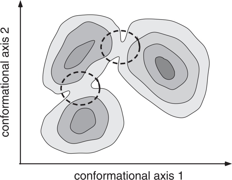
Computer simulation is now widely used to explore the biomolecular conformational space. Free-energy (or energy) landscape is an important quantity obtainable from the simulation. The landscape provides distribution of thermodynamically stable states (low-energy basins) and pathways connecting the stable states. When the sampling is achieved in a wide conformational space, the landscape can be a road map for large-scale motions such as protein folding or protein-ligand binding1–5. Figure 1 shows schematically the landscape, where the conformation passes through regions circled by broken lines, when an inter-basin transition occurs.

Figure 1.

Schematic drawing for free-energy (or energy) landscape. Three low-energy basins are shown with iso-free-energy contour lines, and broken-line circles indicate bottlenecks that connect the low-energy basins.

To accurately estimate the free-energy difference between the low-energy basins, the conformational sampling should substantialize a number of transitions among the low-energy basins. However, when narrow pathways (bottlenecks) connect the low-energy basins, the frequency of transitions decreases, and the conformational sampling takes a long computing time to estimate accurately the probability (free energy) of each basin. Thus, generally, the computing time for the accurate free-energy estimation increases with narrowing the bottlenecks because the bottlenecks prevent inter-basin traveling. This difficulty lies in many sampling problems of biomolecular systems.

A generalized ensemble (GE) method, such as multi-canonical sampling6–10 or adaptive umbrella sampling11,12, generates an even (i.e. flat) probability distribution along a reaction coordinate. The flatness ensures that the conformational space is sampled widely along the reaction coordinate. In other words, the sampling is enhanced along the reaction coordinate. Thus, one may imagine that the GE method can cause the passing through the bottlenecks effectively. However, we have shown that a fairly performed GE method provides even worse sampling efficiency than a conventional method when the conformational space on the reaction coordinate becomes narrow where the entropy suddenly decreases (i.e., the bottleneck appears on the pathway)13. Even the reaction coordinate is well designed so that the conformational changes along the reaction coordinate provide natural passage through the bottleneck, the conformation may be sluggish for long time in a basin before detecting the bottleneck.

In this study, we introduce a virtual state in the conformational space to ease passing the bottlenecks. Although this method is developed for sampling the biological systems, here we apply it to a simple system, which consists of two basins connected by a bottleneck. Because of the simplicity of the system, the free energies of the basins are computable analytically. We perform two Monte Carlo (MC) simulations called a “real-state MC” and a “virtual-state coupled MC”. The real-state MC is a conventional sampling method without the virtual state. In the virtual-state coupled MC, the virtual state covers the bottleneck. We show that the virtual state considerably enhances the inter-basin round trips.

Methods

Figure 1 is a scheme for the free-energy landscape of a biological system: See also Figure 1b of Ref. 3, which is the free-energy landscape of a β-hairpin peptide in explicit water. Thus, to increase the accuracy of the free energies for the low-energy basins, frequency of passing through the bottlenecks should be increased. To develop a useful method, we introduce a simple model explained below. A benefit of the simple model is that one can estimate analytically the free energies of the basins. We impose an important requirement on the model: a transition among the low-energy basins occurs through a narrow pathway. By varying the narrowness of the pathway, we can assess how our method is effective.

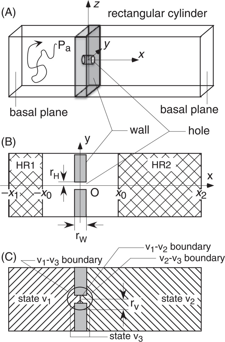
Figure 2 is the simple model, where the inner cavity of a rectangular cylinder is divided into two regions by a wall, and a narrow hole (circular cylinder-shaped hole) is pierced at the center of the wall (see Fig. 2A and B). The two wide regions, denoted as “state v₁” and “state v₂” in Figure 2C, resemble the low-energy basins, and the narrow hole does the bottleneck. A particle P_a is confined inside a rectangular cylinder and moves during a simulation to estimate free energies of the states v₁ and v₂. Thickness of the wall and radius of the hole are denoted as r_W and r_H, respectively (see Fig. 2B). We define a cartesian coordinate system (see Fig. 2) so that the x-axis is the rectangular cylinder axis. The y-axis is parallel to one side of the basal planes of rectangular cylinder and the z-axis to the other side: The origin is set at the body center of the hole (i.e., the body center of the wall). The basal planes for states v₁ and v₂ are defined by x=−x₁ (x₁>0) and x =−x₂ (x₂>0), respectively. The position of P_a is referred as to r = [x, y, z]. For simplicity, we set the potential energy to be constant in the movable region of P_a. Therefore, the free-energy barrier caused by the hole is purely an entropic barrier.

Figure 2.

(A) Overview of system. Winding line illustrates motion of particle P_a. (B) Intersection of the system (panel A) on the x-y plane. (C) Location of the virtual state v₃.

First, we performed a conventional MC simulation and estimated numerically the volumes of the states v₁ and v₂, which are denoted V_v1 and V_v2, respectively. We call this sampling “real-state MC”. Since the potential energy is constant, P_a can move unconditionally in the movable region. To count the round trips of P_a between v₁ and v₂, we introduced two regions, HR1 and HR2 (see netted areas in Fig. 1B), expressed by inequalities x≤−x₀ and x≥x₀ (x₀>0), respectively. After P_a visits HR1 (or HR2), we wait till P_a returns to HR1, during which P_a visits HR2 at least once. We count this move as a round trip. When P_a has returned to HR1 without visiting HR2 (even with visiting state v₂), this move is incomplete as a round trip. Then we wait further till P_a returns after visiting HR2. We denote the number of round trips from a long simulation as N_RT.

Analytical values for V_v1 and V_v2 are given as:

$$V_{\mathit{vi}}^{\text{ana}}=S\left(x_i-h_{\text{W}}/2\right)+\pi r_{\text{H}}^2{r}_{\text{W}}/2,\hspace{0.17em}\hspace{0.17em}\hspace{0.17em}\hspace{0.17em}\hspace{0.17em}\hspace{0.17em}\hspace{0.17em}\left(i=1,2\right)$$ (1)

where S is the area of the bases planes. The free-energy difference between v₁ and v₂ is: $\Delta F=F_{v2}-F_{v1}=-\text{ln}\left[V_{v2}^{\text{ana}}/V_{v1}^{\text{ana}}\right]$. We did not involve temperature in this expression by setting as k_BT = 1, because the potential energy is always constant in the movable region (i.e., V_v1 and V_v2 are independent of temperature). To check the convergence of sampling, we introduce a quantity, volume-ratio convergence, as:

$$C\left(t\right)=\frac{V_{v2}^{\text{num}}/V_{v1}^{\text{num}}}{V_{v2}^{\text{ana}}/V_{v1}^{\text{ana}}},$$ (2)

where $V_{vi}^{\text{num}}$ is the numerically estimated volume for state v_i using a partial simulation trajectory from 0 to t steps. We denote a partial trajectory from t₁ to t₂ steps as I[t₁, t₂]. Practically, $V_{vi}^{\text{num}}$ is replaced by the number of snapshots where P_a exists in v_i in I[0, t].

Next, we introduce a spherical state v₃ centered at the coordinate origin with radius of r_V (Fig. 1C), where the left half (x<0) of v₃ overlaps with v₁, and the right half (x ≥0) with v₂. Therefore, v₃ is not a substantial state separated from v₁ and v₂ but a virtual state. Here, we introduce a virtual-state coupled MC simulation as follows: Suppose that P_a starts from a position in state v₁. During an interval I [0, Δt], we confine P_a to stay in v₁: When P_a is passing the v₁–v₂ boundary, this move is rejected, although P_a can pass the v₁–v₃ boundary freely. If P_a is inside of the v₁–v₃ boundary at the last step of I[0, Δt], P_a may transition to v₃ with a transition probability of p_1→3 (the actual values for the transition probability is given later). Note that this inter-state transition alters the attribution of P_a (i.e. the state specifier) from v₁ to v₃ without changing the position of P_a in the rectangular cylinder. If P_a is outside the v₁–v₃ boundary at the last snapshot, no transition occurs. The particle P_a is confined again in v₁ during the next interval I[Δt, 2Δt], and the state transition is examined at the last step of I[Δt, 2 Δt].

Once the inter-state transition (v₁→v₃) has been accepted at the end of I[0, Δt], then P_a is confined in v₃ during the interval of I[Δt, 2Δt]. Now, P_a can pass the v₁–v₂ boundary freely. However, moves toward outside of the v₁–v₃ and v₂–v₃ boundaries are rejected. At the last step of I[Δt, 2Δt], the state transition is examined as follows: P_a may return back to v₁ with a probability of p_3→1 when P_a is in the region of x<0. On the other hand, P_a may transition to v₂ with a probability of p_3→2 when P_a is in the region of x>0. Suppose that P_a has transitioned to v₂. Then P_a is confined in v₂ during the interval of I[2Δt, 3Δt], where P_a can pass the v₂–v₃ boundary freely, but moves passing the v₁–v₂ boundary are rejected. At the last step of I[2Δt, 3Δ], P_a may transition to v₃ with a transition probability of p_2→3 when P_a is in the region of r≤ r_V, where r = [x²+y²+z²]^1/2. Otherwise, P_a stays in v₂ for the next interval I[3Δt, 4Δt]. By this way, the inter-state transition is examined at steps n Δt (n=1, 2, ...).

Since the motion of P_a from r to r′ within v_i is unconditionally accepted, a long simulation yields an equation:

$$P\left(\mathit{r},v_i\right)=P\left({\mathit{r}}^{\mathit{\prime }},v_i\right)=\mathit{cons},$$ (3)

where P(r, v_i) is the probability distribution function of P_a at position r in v_i. An inter-state transition from v_i to v_j at a position r is controlled by a transition probability p_i→j. Then, the long simulation yields an equation:

$$\frac{P\left(\mathit{r},v_i\right)}{P\left(\mathit{r},v_j\right)}=\frac{p_{j\to i}}{P_{i\to j}}$$ (4)

Combining Eqs. 3 and 4, the probability distribution function satisfies the following equation:

$$\begin{array}{ll}\frac{P\left({\mathit{r}}_1,v_1\right)}{P\left({\mathit{r}}_2,v_2\right)}=\hfill & \frac{P\left({\mathit{r}}_1,v_1\right)P\left({\mathit{r}}_1,v_3\right)P\left({\mathit{r}}_2,v_3\right)}{P\left({\mathit{r}}_1,v_3\right)P\left({\mathit{r}}_2,v_3\right)P\left({\mathit{r}}_2,v_2\right)}\hfill \\ \hfill & =\frac{p_{3\to 1}}{p_{1\to 3}}\frac{p_{2\to 3}}{p_{3\to 2}}\hfill \end{array}$$ (5)

where r₁ and r₂ are arbitrary positions in v₁ and v₂, respectively. Equation 5 indicates that the states v₁ and v₂ are indirectly linked via the virtual state v₃.

We note that Eq. 5 is not an equation to determine the absolute values for the inter-state rate constants. Equation 5 can be rewritten as:

$$\frac{P\left({\mathit{r}}_1,v_1\right)}{P\left({\mathit{r}}_2,v_2\right)}=\frac{p{\prime }_{3\to 1}}{p{\prime }_{1\to 3}}\frac{p{\prime }_{2\to 3}}{p{\prime }_{3\to 1}}$$ (6)

where the inter-state transition probabilities are redefined as:

$${P^{\prime }}_{i\to j}=k{p}_{i\to j},$$ (7)

where the coefficient k is any positive value. With increasing k, the rate constant increases, and the simulation length to reach equilibrium becomes short. In MC scheme, then, the largest rate constant (the quickest convergence) may be result from p_i→j = 1. The parameter Δt also changes the rate constants: the larger the Δt, the longer the simulation length to obtained an equilibrated probability distribution function.

Based on the above discussion, the parameter set of [p_i→j, Δt]=[1, 1] may be the best to speed up the round trips. Note that this parameter set is similar with the simulation condition of the real-state MC (i.e., the conventional MC). In fact, we show below that the smaller the Δt, the quicker the convergence. However, against our better instincts, the larger the p_i→j, the worse the sampling efficiency for a narrow-hole system.

Results and discussion

We set the system parameters (non-dimensional quantities) as: S=2.0²=4, r_W= 0.2, x₁= 1.0, x₂= 2.0 and x₀= 0.5. Quantities r_H, Δt, and p_i→j are specific to the virtual state. We examined several values for r_H and Δt: r_H= {0.005, 0.01, ..., 0.16}={d×2⁰, d×2¹, ..., d×2⁵} where d=0.005, and Δt= {1, 10, ..., 100000}={10⁰, 10¹, ..., 10⁵}. For simplicity, the transition probabilities from the virtual state to the real states are set to a single value p_t, and those from the real states to the virtual state to 1.0: I.e., p_3→1 = p_3→2= p_t (0< p_t≤ 1) and p_1→3= p_2→3 = 1.0. We examined ten p_t values as: p_t= {2⁻⁹, 2⁻⁸, ..., 2⁻¹, 1}. The size of the virtual state r_V was set to 0.3. The total MC length (number of trials to move P_a) is 5 × 10¹¹ steps for all simulations.

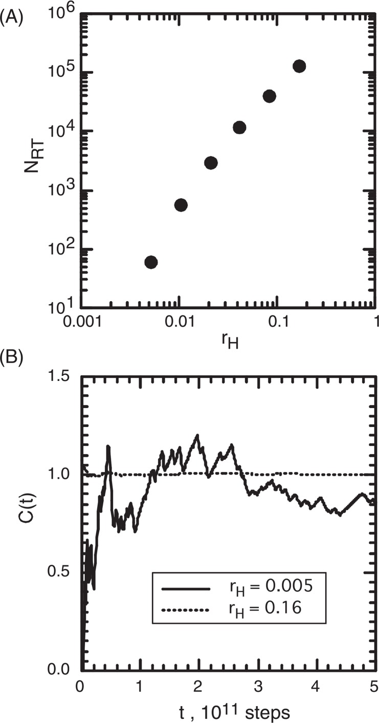
In the real-state MC, N_RT rapidly decreased with decreasing r_H (Fig. 3A). Figure 3B demonstrates the volume-ratio convergence C(t) for r_H= 0.16 and r_H= 0.005. The convergence was quick for r_H= 0.16 and slow for r_H= 0.005.

Figure 3.

Real-state MC. (A) Relation between r_H and N_RT, and (B) volume-ratio convergence, C(t), for two r_H values.

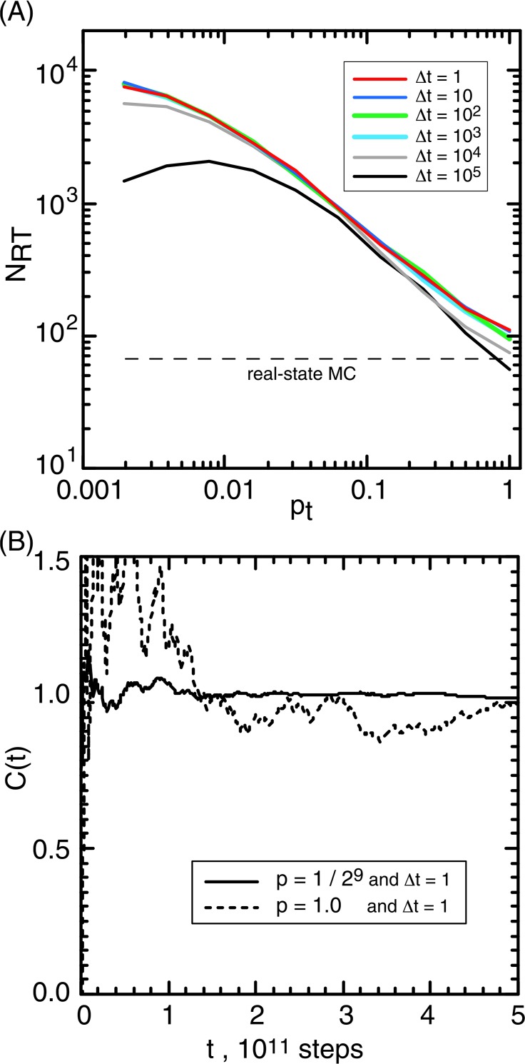
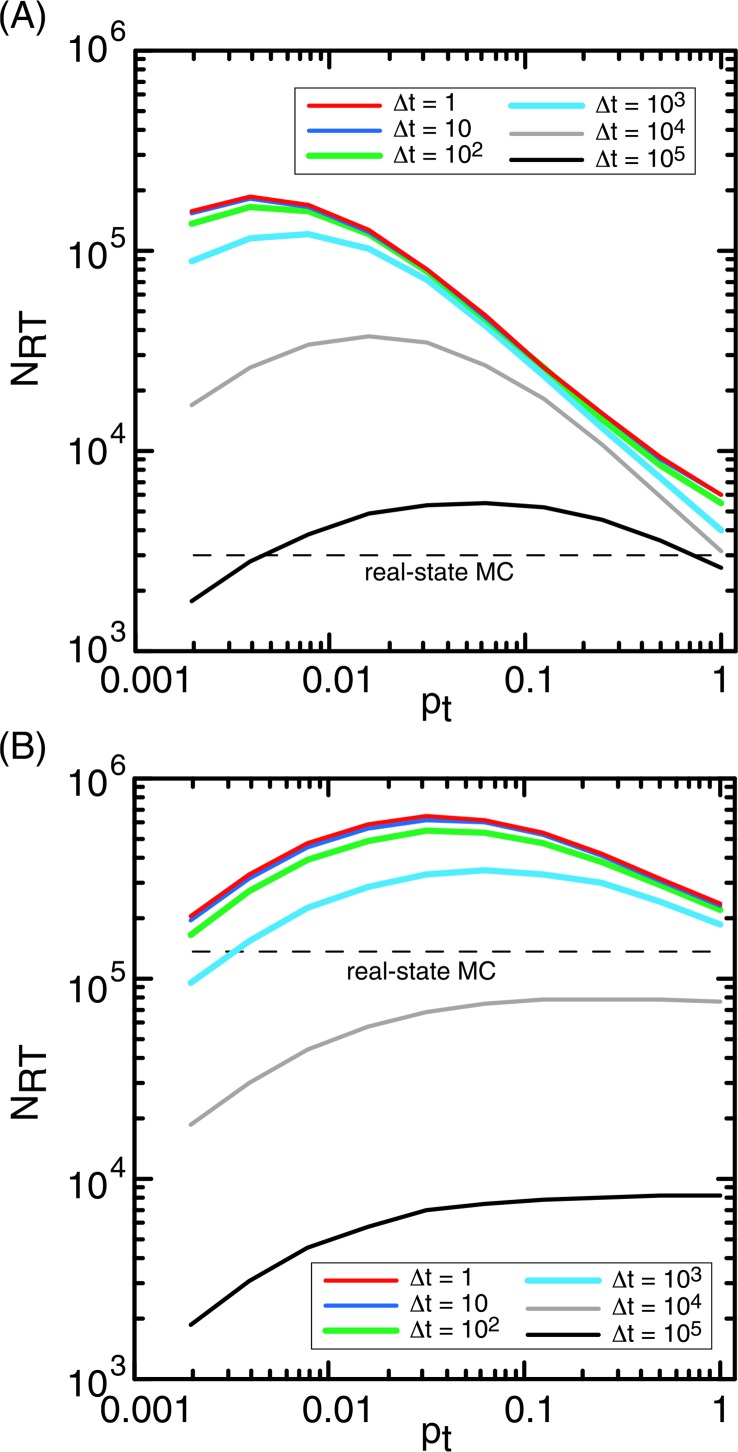
Current study presents a recipe to enhance the sampling by introducing the virtual state for a narrow-hole system. The p_t–N_RT relation (Fig. 4A) for the narrowest-hole system (r_H= 0.005) at various Δt manifests that the virtual state enhances the sampling because N_RT is larger than that from the real-state MC (broken line). The only exception was found at [p_t, Δt]=[1, 10⁵]. For Δt≤10⁴, N_RT increased monotonically with decreasing p_t. The highest efficiency was found at p_t= 2⁻⁹, where N_RT was about 100 times larger than that from the real-state MC. Figure 4B plots C(t) from [p_t, Δt] = [2⁻⁹, 1] and [1, 1]. The convergence was quick for p_t= 2⁻⁹ and slow for p_t= 1. The mechanism for the enhancement is simple: With decreasing p_t, the probability P(r, v₃) of P_a in the virtual state increases, and accordingly the hole-passing chance increases.

Figure 4.

Virtual-state coupled MC for r_H = 0.005. (A) Relation between p_t and N_RT at the various Δt. Broken line represents N_RT from real-state MD. (B) Volume-ratio convergence, C(t), from simulations with [p_t, Δt] = [2⁻⁹, 1] and [1, 1].

The black solid line (Δt=10⁵) of Figure 4A had different behavior from the other lines (Δt ≤10⁴): N_RT had a peak at p_t= 2⁻⁷. Let us consider a situation that p_t falls to zero (p_t → 0). In this extremity, N_RT should decay to zero (N_RT → 0) because P_a cannot escape from v₃ once P_a is trapped in v₃. Then, we get two inequalities: dN_RT/dp_t|_pt=0 >0 and dN_RT/dp_t|_pt=1<0. These inequalities result in that N_RT has a peak. The N_RT showed no peak for Δt≤10⁴ because the peak position is below p_t= 2⁻⁹. Here, one may raise a question: Why does the peak position for Δt =10⁵ was larger than those for the other Δt? This is because increment of Δt decreases the inter-state transitions (the rate constants). In this regime, a large p_t (transition probability from v₃ to v₁ or v₂) plays a role of enhancer for inter-state transitions. Accordingly, the peak position shifts positively.

The positive shift of the peak position is clearly shown for a middle hole r_H= 0.02 (Fig. 5A): All curves had a peak, and the peak position shifted positively with increasing Δt. Figure 5B demonstrates the p_t−N_RT relation for the largest hole (r_H= 0.16), where the peak position was merge into the edge of p_t (p_t= 1) for Δt≥10⁴.

Figure 5.

Relation between p_t and N_RT for r_H = 0.02 (A) and r_H = 0.16 (B).

The virtual-state coupling is readily applicable to GE methods, such as multicanonical or adaptive umbrella sampling. The GE enhances the sampling along a reaction coordinate x with introducing an effective potential energy E_eff = E+k_BT ln[P_c(x, T)], where E is the original potential energy, P_c(x, T) a canonical distribution of x at temperature T, and k_B the Boltzmann constant. The reaction coordinate is a function of position (or conformation) r: x=x(r). The positional transition probability from r₁ to r₂ is simply given by exp[−ΔE_eff/k_BT], where ΔE_eff = E_eff (x(r₂)) − E_eff (x(r₁)). The phase point fluctuating in the entire conformational space may spend a long time before running into the narrow bottleneck8. One can set the virtual state covering the bottleneck, where the virtual volume is larger than the bottleneck size. Then, the chance that the phase point finds the bottleneck increases. In the virtual state, the phase point can find bottleneck readily because the phase point is confined in the virtual state for a while.

We note that the current method is expandable readily to molecular dynamics (MD) by computing an effective force ${\mathit{f}}_i^{\text{eff}}$ acting on atom i as: f_i = −grad[E_eff (x, T)]9. With introducing the virtual state, a canonical MD simulation at temperature T with ${\mathit{f}}_i^{\text{eff}}$ becomes virtual-state coupled multi-canonical or adaptive umbrella sampling. Conformational changes in each time interval Δt are done by MD scheme, and the inter-state transitions examined at the end of time intervals (t =nΔt) are achieved by MC scheme.

In the present study, the bottleneck position in the conformational space is known in advance. However, the bottleneck position is generally unknown a priori. Then, before introducing the virtual state, pre-sampling is required, which may be a “real-state” multicanonical or adaptive umbrella sampling. In general, shape and volume of the virtual state are arbitrary depending on the system.

The current model (Fig. 2) was defined in the three-dimensional space. Then, one may doubt if the current method is useful for biological systems, because the biological systems are defined in a high-dimensional space. However, as shown in all-atom model of polypeptides1–5, the bottlenecks are well identified by projecting the high-dimensional distribution in a low-dimensional (2D or 3D) conformational space.

Last, we note that the virtual state acts as a lens to view the probability distribution function at the bottleneck. To increase the events passing through the bottleneck, we set p_t to be small, which makes the probability distribution for the virtual state large. Thus, the virtual-state coupled sampling can be used to estimate both free energies of major basins and the bottlenecks (i.e., free-energy barriers).

References

- 1.Ono S, Nakajima N, Higo J, Nakamura H. The multicanonical weighted histogram analysis method for free energy landscape along structural transition paths. Chem Phys Lett. 1999;312:247–254. [Google Scholar]
- 2.Higo J, Galzitskaya OV, Ono S, Nakamura H. Energy landscape of a β-hairpin peptide in explicit water studied by multicanonical molecular dynamics. Chem Phys Lett. 2001;337:169–175. [Google Scholar]
- 3.Kamiya N, Higo J, Nakamura H. Conformational transition states of a β-hairpin peptide between the ordered and disordered conformations in explicit water. Protein Sci. 2002;11:2297–2307. doi: 10.1110/ps.0213102. [DOI] [PMC free article] [PubMed] [Google Scholar]
- 4.Kamiya N, Mitomo D, Shea J-E, Higo J. Folding of the 25 residue Aβ(12–36) peptide in TFE/Water: Temperature dependent transition from a funneled free-energy landscape to a rugged one. J Phys Chem B. 2007;111:5351–5356. doi: 10.1021/jp067075v. [DOI] [PubMed] [Google Scholar]
- 5.Higo J, Nishimura Y, Nakamura H. A free-energy landscape for coupled folding and binding of an intrinsically disordered protein in explicit solvent from detailed all-atom computations. J Am Chem Soc. 2011;133:10448–10458. doi: 10.1021/ja110338e. [DOI] [PubMed] [Google Scholar]
- 6.Berg BA, Neuhaus T. Multicanonical ensemble: A new approach to simulate first-order phase transitions. Phys Rev Let. 1992;68:9–12. doi: 10.1103/PhysRevLett.68.9. [DOI] [PubMed] [Google Scholar]
- 7.Hansmann UHE, Okamoto Y. Prediction of peptide conformation by multicanonical algorithm: New approach to the multiple-minima problem. J Comp Chem. 1993;14:1333–1338. [Google Scholar]
- 8.Kidera A. Enhanced conformational sampling in Monte Carlo simulations of proteins: application to a constrained peptide. Proc Natl Acad Sci USA. 1995;92:9886–9889. doi: 10.1073/pnas.92.21.9886. [DOI] [PMC free article] [PubMed] [Google Scholar]
- 9.Nakajima N, Nakamura H, Kidera A. Multicanonical ensemble generated by molecular dynamics simulation for enhanced conformational sampling of peptides. J Phys Chem B. 1997;101:817–824. [Google Scholar]
- 10.Iba Y, Chikenji G, Kikuchi M. Simulation of Lattice Polymers with multi-self-overlap ensemble. J Phys Soc Jpn. 1998;67:3327–3330. [Google Scholar]
- 11.Paine GH, Scheraga HA. Prediction of the native conformation of a polypeptide by a statistical-mechanical procedure. I. Backbone structure of enkephalin. Biopolymers. 1985;24:1391–1436. doi: 10.1002/bip.360240802. [DOI] [PubMed] [Google Scholar]
- 12.Mezei M. Adaptive umbrella sampling: Self-consistent determination of the non-Boltzmann bias. J Comp Phys. 1987;68:237–248. [Google Scholar]
- 13.Higo J, Ikebe J, Kamiya N, Nakamura H. Enhanced and effective conformational sampling of protein molecular systems for their free energy landscapes. Biophys Rev. 2012;4:27–44. doi: 10.1007/s12551-011-0063-6. [DOI] [PMC free article] [PubMed] [Google Scholar]