Mapping of Craniofacial Traits in Outbred Mice Identifies Major Developmental Genes Involved in Shape Determination

Abstract

The vertebrate cranium is a prime example of the high evolvability of complex traits. While evidence of genes and developmental pathways underlying craniofacial shape determination is accumulating, we are still far from understanding how such variation at the genetic level is translated into craniofacial shape variation. Here we used 3D geometric morphometrics to map genes involved in shape determination in a population of outbred mice (Carworth Farms White, or CFW). We defined shape traits via principal component analysis of 3D skull and mandible measurements. We mapped genetic loci associated with shape traits at ~80,000 candidate single nucleotide polymorphisms in ~700 male mice. We found that craniofacial shape and size are highly heritable, polygenic traits. Despite the polygenic nature of the traits, we identified 17 loci that explain variation in skull shape, and 8 loci associated with variation in mandible shape. Together, the associated variants account for 11.4% of skull and 4.4% of mandible shape variation, however, the total additive genetic variance associated with phenotypic variation was estimated in ~45%. Candidate genes within the associated loci have known roles in craniofacial development; this includes 6 transcription factors and several regulators of bone developmental pathways. One gene, Mn1, has an unusually large effect on shape variation in our study. A knockout of this gene was previously shown to affect negatively the development of membranous bones of the cranial skeleton, and evolutionary analysis shows that the gene has arisen at the base of the bony vertebrates (Eutelostomi), where the ossified head first appeared. Therefore, Mn1 emerges as a key gene for both skull formation and within-population shape variation. Our study shows that it is possible to identify important developmental genes through genome-wide mapping of high-dimensional shape features in an outbred population.

Author Summary

Formation of the face, mandible, and skull is determined in part by genetic factors, but the relationship between genetic variation and craniofacial development is not well understood. We demonstrate how recent advances in mouse genomics and statistical methods can be used to identify genes involved in craniofacial development. We use outbred mice together with a dense panel of genetic markers to identify genetic loci affecting craniofacial shape. Some of the loci we identify are also known from past studies to contribute to craniofacial development and bone formation. For example, the top candidate gene identified in this study, Mn1, is a gene that appeared at a time when animals started to form bony skulls, suggesting that it may be a key gene in this evolutionary innovation. This further suggests that Mn1 and other genes involved in head formation are also responsible for more fine-grained regulation of its shape. Our results confirm that the outbred mouse population used in this study is suitable to identify single genetic factors even under conditions where many genes cooperate to generate a complex phenotype.

Introduction

Understanding the evolutionary processes that have generated and maintained morphological diversity in nature is a long-standing goal in biology. The cranium and mandible of vertebrates is a good example of such diversity. The fact that the cranial and mandible bones have to be integrated with the brain and sensory systems, as well as with the respiratory and digestive systems, makes this structure a prime example of both high integration and high evolvability.

Although information about genes and developmental pathways involved in shape determination keeps accumulating, we are far away from understanding the genotype-phenotype map translating genetic variation into craniofacial shape variation [1]. To approach this question, here we aim to identify the genetic factors underlying such morphological differences.

Previous experimental work has explored the genetic basis of craniofacial variation in a range of species, including Darwin’s finches [2–4], cichlids [5,6], dogs [7–9], and mice [10–16]. There has also been some recent work on natural facial variation in humans [17–20]. Much of this work has been made possible by developments in geometric morphometrics, which provide the techniques for quantifying subtle shape variation [21]. Combined with increasing availability of genomics resources for mice, this has made possible genome-wide studies of natural shape variation in mice [12].

Early work in mice has focused mainly on the mandible. This is a well-established model for the study of complex traits because mandible shape can be approximated in 2 dimensions [22,23]. Several quantitative trait loci (QTL) studies have investigated mandible shape variation, and have identified several genomic regions underlying 2D variation in this trait, mostly in crosses of inbred laboratory strains [13,24,25]. Although the skull has received less attention due to its higher complexity and the difficulty of defining appropriate phenotypes (2D vs 3D), recently Burgio et al. [15], Pallares et al. [12], and Maga et al. [10] have successfully identified genomic regions underlying 3D skull variation in mice. In our previous study [12], we used genome-wide association (GWAS) based on natural recombinants from a hybrid zone between two subspecies of the house mouse. This enabled us to identify candidate skull and mandible shape loci with much higher resolution than conventional QTL studies in mice (e.g. [10]).

Here, we approach the question from a micro-evolutionary perspective by analyzing within-population shape variation. The utility of studying phenotypic variation at the within-population level is well acknowledged, as it permits one to focus on within-species genetic contributions to phenotypic variation [26]. We use a population of “Carworth Farms White” (CFW) outbred mice, whose suitability for genome-wide mapping was previously described [27–29]. Recently developed genomic resources for this population allow for QTL mapping on autosomal chromosomes (see Methods). The CFW mice were originally derived from a small number of Swiss mice, and have been maintained for dozens of generations as an outbred colony with a large breeding population that avoids crosses between closely related individuals [27,30,31]. Importantly, the mice used in this study show little evidence for population stratification or cryptic relatedness, which simplifies the analysis and interpretation of genetic variation contributing to quantitative traits. The high number of recombination events in the history of this population has resulted in small linkage blocks, which, together with the above mentioned features, result in high mapping resolution [27].

Results

We estimated heritability of craniofacial shape, and assessed support for craniofacial shape and size QTLs at 80,027 autosomal SNPs in 592–720 mice. Skull shape is represented as a 132-dimension vector (coordinates of 44 3D landmarks), and mandible shape is represented as a 39-dimension vector (coordinates of 13 3D landmarks). To make the shape data suitable for QTL mapping, we extracted principal components (PCs) that explain the most variance in skull and mandible shape. Specifically, skull shape was represented by the first 22 PCs that capture 84% of the skull shape variation, and mandible shape was represented by the first 21 PCs accounting for 94% of the variation in mandible shape.

Heritability

Heritability of each skull and mandible PC was calculated using the standard additive polygenic model (S2 and S3 Tables and Fig 1). The heritability values we report here are “SNP heritability” [32]; that is, the estimate of the proportion of phenotypic variance explained by all available SNPs. All skull and mandible PCs exhibit substantial contributions from the additive genetic variance component; only two PCs have heritability values lower than 20%. Mandible size has SNP heritability of 36.4% (95% confidence interval 16.4–56.4), and skull size of 35.4% (15–55.8). To summarize the heritability for mandible and skull shape with a single statistic, we calculated a weighted average of the SNP heritability of individual PCs (see Methods and Fig 1C and 1D). These “total heritability” values are 43.6% for mandible shape and 42.4% for skull shape. This statistic is equal to the proportion of the bar chart that is shaded dark gray in Fig 1C and 1D. We also checked whether the proportion of total phenotypic variation explained by each PC is correlated with our SNP heritability estimates. This correlation is not strong, but significant; mandible, r² = 0.14, p-value = 0.034; skull, r² = 0.16, p-value = 0.034 (Fig 1A and 1B).

Fig 1. SNP heritability of individual PCs.

Correlation between SNP heritability and proportion of variation explained by the PC is shown for (a) mandible and (b) skull. Grey dots represent PCs. In (c) and (d), numbers above the bars indicate the proportion of each bar that is colored dark grey, this is the SNP heritability of each PC. The error bars give standard error of the SNP heritability estimates.

Chromosomal partition of the variance

Partitioning the variance by chromosome shows almost all chromosomes contribute to shape variation (Fig 2). We find also a correlation with chromosome size, as expected, but this is only statistically significant for mandible shape (Fig 2B). In our previous study we found a highly significant correlation for both, mandible and skull shape [12]. The weaker correlation in the present study is likely due to lower and somewhat uneven marker coverage, which is in itself not strongly correlated with chromosome length (S2 Fig). In particular, chromosome 16 is underrepresented with respect to marker coverage; the fact that this chromosome contributes very little to the phenotypic variance (Fig 2) could be due to technical limitations regarding SNP identification, or to this chromosome indeed harboring little variation.

Fig 2. Chromosomal partition of the variance.

These plots compare the contribution of each chromosome to (a) mandible and (b) skull shape variation, and how these contributions correlate with chromosome length (in Mb).

Genomic regions associated with craniofacial size and shape

Out of the 22 PCs used to map skull shape, 12 PCs had at least one significant QTL; and out of the 20 PCs used in the mapping of mandible shape, 7 PCs had a significant QTL (see Fig 3 and Tables 1 and 2). 17 QTLs were identified for skull shape variation (Table 1), and eight QTLs for mandible shape variation (Table 2). One QTL was associated with mandible centroid size, and no QTLs were identified for skull centroid size. The shape traits associated with the “peak SNPs” (SNPs with lowest p-value) are depicted in Figs 4 and S4–S8.

Fig 3. Genome-wide scans for (a) mandible and (b) skull.

This plot shows p-values for association with craniofacial phenotypes—22 skull shape PCs, 21 mandible shape PCs and centroid size—at 80,027 candidate SNPs. Since only the smallest p-values are visible from this plot, p-values for individual PCs are drawn in separate plots; see S9 and S10 Figs. The associated phenotype (PC or centroid size) is indicated for each QTL. The blue line represents an approximate genome-wide significance threshold, 1e-6 (-log(p) = 6); the actual threshold we used to determine significance of the p-values is different for each phenotype (average–log(p) = 6.05, min = 5.95, max = 6.16). *To improve visualization, the p-value shown in the Figure is larger than the actual p-value; the actual p-values are PC4* -log(p) = 26.6, PC3* -log(p) = 14.8.

Table 1. SNPs associated with skull phenotypes (PCs).

Columns of the table show the SNP with the lowest p-value per QTL, its base-pair position, p-value calculated in GEMMA, and the proportion of total skull shape variation explained by the SNP (%varSkull).

Region	Skull	Chr	Pos	SNP	p-value	%varSkull	Candidate genes
1	PC1	11	32367260	rs258942042	9.13E-07	0.75	Sh3pxd2b
2	PC1	13	110231696	rs245694506	3.93E-07	0.86	Rab3c, Plk2, Pde4d
3	PC2	8	80889309	rs228570244	7.54E-07	0.62	Gab1, Inpp4b
4	PC3	5	111328046	rs33702397	2.18E-27	2.05	Mn1
5† **	PC4	9	99713529	rs30491142	9.69E-09	0.44	Cldn18
6**	PC5	2	33284278	rs27194486	5.74E-07	0.35	Lmx1b
7† **	PC5	9	98588137	rs13466556	4.35E-09	0.56	Foxl2
8*	PC6	5	111626960	rs254983846	1.53E-08	1.27	Mn1
9*	PC6	19	4165856	rs37378594	3.24E-08	0.48	-
10† *	PC7	13	31734894	cfw-13-31734894	4.00E-09	0.53	Foxf2, Foxc1
11† *	PC8	3	98931976	rs30352013	4.71E-07	0.38	Tbx15
12*	PC8	5	110918274	rs227631022	2.63E-09	1.15	Mn1
13	PC12	11	32423285	rs26862534	9.48E-07	0.40	Sh3pxd2b
14*	PC19	11	95634099	rs26992385	8.83E-07	0.20	-
15	PC20	2	83096089	rs46747509	9.08E-07	0.61	Itgav
16*	PC20	11	94881746	rs50079241	1.29E-07	0.47	Col1a1, Dlx3
17*	PC22	15	11384042	rs31584944	9.85E-07	0.25	Npr3

Principal component (PC). %varSkull is the proportion of variation in skull shape explained by the SNP. This value was calculated in a multivariate regression of shape on the SNP genotype. The candidate genes were identified based on their role in bone morphogenesis (see methods). Empty cells (-) mean no compelling candidate gene emerged. The total set of genes in the QTL regions is shown in S4Table

† Regions that overlap with Maga et al 2015

* Regions that overlap with Attanasio et al 2014 using a window of 500Kb around the focal SNP

** Regions that overlap with Attanasio et al 2014 using a window of 1Mb around the focal SNP

Table 2. SNPs associated with mandible phenotypes (PCs).

Columns of the table show the SNP with the lowest p-value per QTL, its base-pair position, p-value calculated in GEMMA, and the proportion of total skull shape variation explained by the SNP (%varMand).

Region	Mandible	Chr	Pos	SNP	p-value	%varMand	Candidate genes
1*	PC4	5	111018365	rs33217671	1.66E-15	1.28	Mn1
2*	PC7	5	111426493	rs33614268	7.63E-10	1.44	Mn1
3*	PC7	11	35295119	rs28219152	2.66E-08	0.44	-
4† **	PC8	9	99595168	rs29977169	6.18E-07	0.27	Cldn18
5	PC12	6	107312800	rs36343125	7.93E-07	0.22	-
6	PC15	14	98935309	rs237064333	1.68E-08	0.22	Klf5
7‡ **	PC19	11	96261688	rs233696367	8.25E-07	0.31	Hoxb cluster
8†	PC20	4	90510654	rs221759350	6.48E-07	0.26	-
9*	Centroid size	1	153481175	rs32618422	5.96E-09	5.08	-

Principal component (PC). Centroid size (CS). %varMand is the proportion of variation in mandible shape explained by the SNP. This value was calculated in a multivariate regression of shape on the SNP genotype. The candidate genes were identified based on their role in bone morphogenesis (see methods). Empty cells (-) mean no clear candidate gene emerged. The total set of genes in the QTL regions is shown in S5 Table

† Regions that overlap with Maga et al 2015

‡ Region that overlap with Pallares et al 2014

* Regions that overlap with Attanasio et al 2014 using a window of 500Kb around the focal SNP

** Regions that overlap with Attanasio et al 2014 using a window of 1Mb around the focal SNP

Fig 4. Changes in mandible (a-c) and skull (d-g) shape associated with the SNPs of largest effect.

SNP rs33702397 explains 2% of skull shape variation, and rs33614268 explains 1.4% of mandible shape variation. The sample mean shape is depicted in grey (dotted line). In orange (continuous line) is the mean shape associated to the SNP effect, scaled 10x. For mandible, (a) lateral, (b) frontal, and (c) dorsal views are shown. For skull, (d) dorsal, (e) frontal, (f) lateral, and (g) ventral views are shown. Dots and numbers represent relevant landmarks for each view.

In some cases multiple QTLs were found in the same chromosome (chr2, 5, 9, 11, 13) but associated with different PCs (Fig 3). Four QTLs were associated with more than one PC; interestingly, two of them were associated with PCs from skull and mandible (chr5 and chr9).

Together the 17 QTLs identified for skull shape explain 11.4% of skull variation. The 8 QTLs for mandible shape together explain 4.4% of mandible variation. The effect size of individual SNPs ranges from 0.02 to 1.13% of the total phenotypic variation (Fig 5 and Tables 1 and 2). The single QTL found for mandible size explains 4.1% of size variation.

Fig 5. Effect size of peak SNPs (lowest p-value in each QTL) associated with (a) mandible and (b) skull shape.

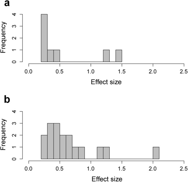
Together the peak SNPs explain 11.4% of variation in skull shape, and 4.4% of variation in mandible shape.

Candidate genes

We compiled a list of 115 protein-coding genes within the craniofacial shape QTLs (S4 and S5 Tables). For most of the regions compelling candidate genes could be identified based on previously reported craniofacial phenotypes or previous evidence for a role in bone morphogenesis. Table 3 lists the functional information available for these genes. Most candidate genes listed in this table are transcription factors or known regulators of developmental signaling cascades.

Table 3. Previously published findings supporting involvement of candidate genes in craniofacial phenotypes, in alphabetic order by gene.

Gene	Biochemical function	Developmental function	Mutant phenotype	Human disease association
Cldn18	structural component of tight junctions	expressed in osteoblasts [33]; regulates bone resorption and osteoclast differentiation via the RANKL signaling pathway [34]	decreased total body bone mineral density, trabecular bone volume, and cortical thickness [35]
Col1a1	extracellular matrix protein	main component of connective tissues	shows decreased bone volume/tissue volume and reduced trabecular number; exhibits mechanically weak, brittle, fracture-prone bones [36]	osteogenesis imperfecta, a human syndrome characterized by bone fragility; subjects also show craniofacial alterations and deficient osteogenesis [37,38]
Dlx3	transcription factor with homeobox domain	regulates adult bone mass and remodeling [39,40]	branchial arch specification and craniofacial defects [39,41]	tricho-dento-osseos syndrome (TDO) in humans, characterized by increased bone mineral density, craniofacial defects, and abnormal teeth and hair [42]
Foxc1	transcription factor with forkhead domain	interacts with BMP signaling and Msx2 to control calvarial bones osteogenesis [43–45] and with Fgf8 to regulate the patterning of the mammalian jaw [46]	congenital hydrocephalus with calvaria bones absent [47]	Axenfeld-Rieger syndrome, includes among other defects abnormalities in teeth and jaw [48]
Foxl2	transcription factor with forkhead domain	among other functions, is also active in cranial neural crest cells and cranial mesodermal cells [49]	muscular and skeletal craniofacial malformations [49,50]	blepharophimosis, ptosis, epicanthus inversus syndrome (BPES) characterized by eyelid and craniofacial malformations and ovarian failure [51]
Gab1	adaptor molecule with pleckstrin domain	involved in intracellular signaling cascades of EGFR and FGFR and cytokine receptors [52]; regulates osteoblast maturation and mineralization in long bones in mice [53]	embryonic lethal [52]; disruption of its expression in osteoblasts leads to decreased trabecular bone mass with a reduced bone formation rate and a decreased bone resorption [53]
Inpp4b	phosphatase involved in phosphatidylinositol signaling pathways	represses osteoclast differentiation by regulation of the transcription factor Nfatc1 that beside others, regulates Itgav [54,55]	bone loss and osteoporosis [54,55]	BMD variation in pre-menopausal women [54,55]
Itgav	integrin family of transmembrane proteins	heterodimer Itgav-Itgb3 is characteristic of osteoclasts, regulating its apoptosis and the process of bone resorption [56]	various phenotypes, including cleft palate [57]
Klf5	transcription factor with Krüppel-like zinc finger domain	regulates the commitment of ES cells to mesoderm lineage [58], and the epithelial-mesenchymal transition [59]	affects tooth development [60]; when overexpressed calvaria bones are absent and mandible is underdeveloped [61]
Lmx1b	transcription factor with homeobox domain	involved in a variety of developmental processes, including limbs, brain, kidney, eye, and calvarial bones [62]	multiple calvarial defects [63]	Nail-patella syndrome (NPS) including limb defects [63]
Mn1	transcriptional activator	modifies vitamin D [64] and vitamin A receptor mediated transcription [65] in the context of bone formation and regulates osteoblast development [64,66]	craniofacial defects affecting exclusively membranous bones in the skull [65]	involved in craniofacial deformations [67] and palate cleft syndromes [67,68]
Npr3	natriuretic peptide receptor	among other functions, it isinvolved in differentiation and proliferation of bone cells [69,70]	skeletal-overgrowth syndrome with endochondral ossification defects [69,71]
Rab3c	regulatory GTPase	regulates vesicular trafficking in the cell, is expressed in mouse calvaria osteoblast and is thought to play a role in bone mineralization [72]	in cell culture studies it regulates the formation of the ruffled membrane, the resorptive organelle of the osteoclast [73]
Pde4d	phosphodiesterase specific for cAMP degradation	expressed in calvaria osteoblasts [74]; some splice variants regulate BMP-induced bone formation [74,75]	regulates osteoblast differentiation in vitro by degrading cAMP [74,75]	Acrodysostosis, skeletal syndrome including nasal hypoplasia and skull deformities [76]. BMD variation in humans [77]
Sh3pxd2b	substrate of Src tyrosine kinase	involved in EGF signaling pathway [78] and the formation of podosomes, which are thought to contribute to tissue invasion and matrix remodeling	craniofacial and skeleton malformations in mice [79–81]	syndromes with craniofacial deformities, Frank-Ter Haar syndrome [82], and Borrone dermato-cardio-skeletal syndrome [83]
Tbx15	transcription factor with T-box domain	involved in early endochondral bone development in prehypertrophic chondrocytes of cartilaginous templates [84]	general reduction of bone size and changes of bone shape [84]; droopy-eared mutation in mice [85,86]	Cousin syndrome including craniofacial dysmorphism [87]

Discussion

The number of regions identified in this study, together with the high mapping resolution in the CFW mouse population, demonstrates the feasibility of mapping within-population variation of complex traits like craniofacial shape. Our results also contribute novel biological insights into the genetic architecture and heritability of craniofacial shape in mice.

Genetic architecture of craniofacial traits

Craniofacial shape

Our results support the notion of a highly polygenic architecture for craniofacial shape in mice. Data derived from other approaches also support this conclusion [11,12]. Such a highly polygenic architecture is expected to facilitate evolutionary modulations and transitions since micro-evolutionary changes at the population level can easily become subject of positive selection and their combined effect can generate large changes in the phenotype.

In total, 17 genomic regions were associated with skull shape, and 8 regions were associated with mandible shape; together they explain 11.4% and 4.4% of the total skull and mandible shape variation, respectively. The total SNP heritability was estimated to be 43.6% for skull shape and 42.4% for mandible shape based on models of polygenic variation for the individual PCs. Although reducing the genetic contribution of a complex, multivariate trait to a single number is necessarily an oversimplification, this nonetheless suggests that the majority of the additive genetic variation is not captured by the SNPs that crossed the significant threshold as defined in this study. This, together with the small effect size of individual loci suggests that the number of loci contributing to the fine-tuning of shape are, at least, in the order of hundreds. We expect that this hidden variation would become apparent with larger sample sizes or in other genetic contexts.

We found little overlap in the regions associated with skull and mandible (Table 1). Given the shared developmental origin of the mandible and some parts of the skull, more overlap would have been expected. However, since it appears that the loci identified by genome-wide association analysis constitute only a small proportion of the real number of functionally relevant loci, it is possible that the lack of overlap reflects the difficulty of identifying strong support for genetic variants contributing to highly complex traits.

Principal components representing small (e.g. PC20) as well as large (e.g. PC1) proportions of the total phenotypic variation were found to associate with genetic variants (Table 1). This pattern was also found previously [12,88]. SNP heritability estimates showed that all PCs included in this study have moderate to high additive genetic variation (S2 and S3 Tables and Fig 1) and therefore associations with genomic regions are expected regardless of the amount of phenotypic variation represented by individual PCs. Mapping approaches that do not rely on principal component analysis show that vectors different from PCs are associated with QTLs (see Maga et al. [10]). The fact that many different dimensions of shape variation associate with genetic variation would be an expected consequence of the highly polygenic architecture of craniofacial shape traits.

Craniofacial size

Only one genomic region was significantly associated with mandible size, while no significant associations were found for skull size. Previous studies found up to 23 QTLs associated with mandible size variation [24,25,89], and seven QTLs for skull size variation [10]. Most of these studies are based on mouse lines with a specific contrast in size, i.e. the lines had been selected for large or small size. In our study using a wild-derived population of mice we did not find significant associations with craniofacial size either [12]. Given the large additive genetic variance of craniofacial size in the CFW mice used here, as well as in wild mice [12], the absence of specific associations suggests that the effect size of loci involved in size variation is very small, even smaller than the effect of loci controlling shape, and therefore the power of these two studies was not enough to detect them.

Heritability of morphological traits

The total heritability estimated in this study, ~43% for craniofacial shape and ~36% for craniofacial size, corresponds to SNP heritability estimates. In humans, SNP heritability is considered an underestimate of the narrow sense heritability because it does not take into consideration rare alleles [90]. However, in the CFW population used here, rare alleles are expected to be uncommon due to the bottleneck when the population was started, the limited number of generations since the bottleneck, and the modest effective population size. Thus, SNP heritability estimates in this population may be closer to narrow sense heritability. Using a population of wild derived mice and a 3D approach, craniofacial SNP heritability was estimated as 65% for shape and 72% for size [12].

Using a pedigree of wild caught mice and a 2D approach, the heritability of mandible shape and size was found to be 0.61 and 0.49, respectively (Siahasarvie and Claude, personal communication). Regardless of the method or the experimental design, the heritability estimates for mandible size and shape in mice are high. It remains to be seen if the same pattern is true for the skull; pedigree-derived data need to be collected.

In a recent study of wild soay sheep, the SNP heritability of mandible length was estimated to be 53% [91]. Human studies estimate a narrow sense heritability of ~0.8 for facial morphology [18]. Although more data are needed, a pattern emerges from these studies: the form (i.e. shape and size) of craniofacial structures is a highly heritable trait.

Candidate genes

The resolution achieved here was much higher than the resolution from traditional F₂ crosses. Although the resolution was still not high enough to conclusively pinpoint individual genes, it was nonetheless possible to explore all genes within the QTL regions and often we identified a single candidate gene for which previous relevant phenotypic information existed. Moreover, 77% of the regions overlap with previous studies (see Tables 1 and 2); 7 of them with QTL regions derived from a backcross [10], 19 of them overlap with some of the ~ 4,000 enhancers active during craniofacial development in the mouse [11], and 1 region overlaps with a GWAS using a wild-derived population of mice [12]. Such overlaps cannot be explained by chance only (S3 Fig). Enhancers are DNA sequences that positively regulate the expression of nearby genes; therefore the high overlap with the enhancer dataset could indicate that some of the SNPs identified in this study tag a causal variant located in the regulatory region of the candidate genes.

The possibility of representing visually the shape traits associated with each SNP (see Figs 4 and S4–S8) allows the identification of specific craniofacial regions affected by the candidate genes. This information will become very valuable in future studies exploring the developmental role of such genes in craniofacial shape determination.

Many of the candidate genes are genes with reported craniofacial phenotypes. However, most of them were previously not quantitatively assessed and therefore knowledge of their specific effects on craniofacial shape variation requires a geometric morphometrics analysis of mutant mice. Such an analysis can be done in heterozygous knockout mice for the gene of interest. In this way the genetic alterations and their phenotypic effects are less drastic compared to the knockout of both alleles, and therefore closer to natural variability within populations [92]. Several other genes are new candidates for craniofacial shape determination; they are involved in diverse processes of bone formation but have not been directly implicated in craniofacial development.

We found two pairs of genes involved in the same signaling pathway; Sh3pxd2b and Gab1 are part of the epidermal growth factor signaling pathway–EGF; Sh3pxd2b regulates EGF-mediated cell migration [78], and Gab1 is involved in EGF-mediated cell growth [52]. Mn1 and Cldn18 are involved in the RANK-RANKL-OPG signaling pathway; Mn1 regulates RANKL expression by stimulating RANKL’s promoter [66], and Cldn18 regulates RANKL-induced differentiation of osteoclasts [35].

Among the candidate genes, Mn1 is a particularly interesting one. It was originally discovered for being involved in a myeloid leukemia phenotype and it was therefore named meningioma 1 [93]. This gene has the largest effect size in our screen (Tables 1 and 2) and is associated with many PCs in the skull and in the mandible (regions 4, 8, 12 in Table 1, regions 1 and 2 in Table 2, and S11 Fig), thus being also the most pleiotropic gene in our study. Knockout studies of Mn1 revealed that the leukemia phenotype of the gene is only a by-product of a particular fusion with another gene, while the core function of Mn1 lies in regulating the development of membranous bones of the cranial skeleton [65]. Intriguingly, Mn1 is an orphan gene specific to bony vertebrates (Euteleostomi) (S12 Fig), a taxon characterized by the formation of bones and a suture-structured head skeleton. The origin of such orphan genes is connected to the emergence of evolutionary novelties [94], and the Mn1 knockout phenotype in mouse suggests that it plays a crucial function in the emergence of a vertebrate novelty–the bony head. Hence, Mn1 has the hallmarks of a key gene in the genetic architecture of craniofacial development and shape determination. The fact that it also emerges out of our genome-wide analysis lends credence to the notion that the approach is suitable to detect relevant genes even for highly polygenic phenotypes.

Conclusions

There are long standing discussions about how to deal experimentally with polygenic traits and their implications for understanding the evolution of such traits [95,96]. Genome-wide association studies have certainly moved us forward in this respect. Even relatively simple quantitative phenotypes like human height have a highly polygenic nature [97,98]. Still, when a sufficiently powerful experimental design is used, key regulatory pathways influencing this phenotype can be identified [97,98]. The natural variants of these pathways have individually small effects, but knockouts of these genes can have large effects.

Here we have shown that we have a similar scenario regarding craniofacial shape, which is a complex phenotype with a highly polygenic architecture. It is encouraging to see that even under such seemingly adverse genetic conditions, we can still identify credible candidate genes previously studied in loss of function experiments. This implies that genes occupying central positions in developmental pathways may also be the ones that carry enough natural variation to allow mapping through GWAS. At the same time we identified regions without any previous information related to craniofacial development (skull regions 9 and 14; mandible regions 3, 5, 8 and 9); such discoveries contribute new information to the genetics underlying skull and mandible shape determination, and dedicated efforts should be made to understand the phenotypic effect of the genes and regulatory elements falling in such regions.

Human studies required ~25,000 individuals to explain 3–5% of height variation with genome-wide-significant SNPs [99], and ~250,000 to explain 16% [97]. Using ~5,400 individuals, only 5 loci were significantly associated with facial morphology in humans [18]. We have explained 4–11% of craniofacial variation using only ~700 outbred mice. Given the development of semi-automatic tools to speed up the phenotyping of shape traits (e.g. [100]), it seems feasible to increase both the number of animals involved, as well as to apply these tools to different mapping contexts. Hence, we are becoming more confident that an understanding of the biology behind craniofacial development will become possible.

Materials and Methods

Ethics statement

All procedures were approved by the University of Chicago Institutional Animal Care and Use Committee (IACUC) in accordance with National Institute of Health guidelines for the care and use of laboratory animals.Mapping population Male mice from the CFW mouse colony, maintained by Charles River Laboratories, were used for genome-wide association mapping. Upon their arrival at the University of Chicago, the mice were subjected to behavioral and physiological tests over the course of 2011 and 2012 (additional phenotype data from these tests are included in a separate manuscript that is being prepared for publication). At the end of these experiments, the mice were sacrificed and their heads were stored in ethanol. The average age at the time of sacrifice was 13 weeks (ranging from 12 to 14 weeks). Skulls and mandibles were measured in a subset of 720 mice between 2013 and 2014 at the Max Planck Institute for Evolutionary Biology in Plön, Germany.

Shape phenotyping

Mouse heads were scanned using a computer tomograph (micro-CT—vivaCT 40; Scanco, Bruettisellen, Switzerland) at a resolution of 48 cross-sections per millimeter. Using the TINA landmarking tool [101], 44 three-dimensional landmarks were positioned in the skull, and 13 in each hemimandible (S1 Fig and S1 Table). The semi-automatic landmark annotation extension implemented in the TINA landmarking tool was used to reduce digitation error and accelerate the phenotyping process [100]. The raw 3D landmark coordinates obtained in TINA tool were exported to MorphoJ [102] for further morphometric analyses.

The symmetric component of the mandible and skull were obtained following [103]. In short, for mandible a full generalized Procrustes analysis (GPA) was performed with the landmark configurations of the right and left hemimandibles. The GPA eliminates the variation due to size, location, and orientation of the specimens, and generates a new dataset that only contains shape variation. For each individual, we recorded an average of the right and left resulting configurations, which represents the symmetric component of shape variation. For skull, a mirror image of the landmark configuration of each individual was generated, and a full GPA was performed with the original and mirror configurations. Again, the resulting configurations were averaged to obtain the symmetric component of shape variation. The new landmark coordinates generated by the GPA are called “Procrustes coordinates”.

To define shape features, we computed in MorphoJ principal components (PCs) from the n x 3k covariance matrix of Procrustes coordinates, where n is the number of samples and k is the number of landmarks; 3k represents the number of Procrustes coordinates (n = 590, k = 13 for mandible, and n = 710, k = 46 for skull). PC loadings computed in this analysis define the phenotypes used in the QTL mapping. Differences in age, spanning 2 weeks, did not correlate significantly with shape variation, so we did not use age as a covariate in subsequent analyses.

Bone-mineral density (BMD)

In a separate project that will be presented in more detail in a later publication, areal BMD (aBMD) of the isolated femur was examined. Unexpectedly, we found that CFW mice appear to be predisposed toward abnormally high aBMD. This is a characteristic of the CFW mice that does not appear to be shared with commonly used inbred lab strains. A qualitative analysis of mice with high BMD showed substantial differences in mandible, and modest differences in the skull compared to mice with normal BMD. We therefore assessed covariation of BMD with shape measurements, separately for the skull and the mandible.

For the skull, we found a small correlation between BMD and shape (r² = 1.4%, p(10,000 permutations) < 0.001). However, no individual PC corresponds to these shape differences due to BMD. Therefore, BMD was not used as covariate for skull trait mapping since it would have little to no effect on our ability to map QTLs for skull shape.

For the mandible, there was a stronger correlation between shape and BMD (r² = 6%, p(10,000 permutations) <0.001). BMD accounts for 29% of the variation in the first PC, 8% of the variation in the third PC, but little to no variation in the remaining PCs (maximum r² is 1.4% for PC6). Therefore, we computed mandible shape residuals by removing the linear effect of BMD; we used these residuals as input to the PCA, then PC loadings from this PCA analysis were used as phenotypes in the QTL mapping for mandible shape.

Size phenotyping

The standard measure of size in geometric morphometrics is the centroid size (CS). This is the measure we used for mapping. Centroid size is defined as the square root of the sum of the squared distances of a set of landmarks from the center of gravity or centroid [104]. The CS for mandible was defined as the average of the CS of right and left hemimandible. The skull CS was calculated using all landmarks from right and left sides [103]. All these calculations were done in MorphoJ.

Genotyping

The mice were genotyped using a genotyping-by-sequencing (GBS) approach [105]. In separate work, we have shown that GBS protocols can be used in combination with existing mouse genomics resources and software toolkits to obtain high-quality genotype data at a large number of genetic markers. In short, GBS libraries were prepared by digesting genomic DNA with the restriction enzyme PstI and annealing barcoded oligonucleotide adapters to the resulting overhangs. Samples were multiplexed 12 per lane, and sequenced on an Illumina HiSeq 2500 using single-end 100-bp reads. By focusing the sequencing effort on the Pstl restriction sites, we obtained high coverage at a subset of genomic loci. The 100-bp single-end reads were aligned to the Mouse Reference Assembly 38 from the NCBI database (mm10) using bwa [106]. We used a GBS-adapted version of the “best practices” pipeline of GATK [107–109] to discover variants and call genotypes. For the Variant Quality Score Recalibration (VQSR) step, we calibrated variant discovery against (1) whole-genome sequencing (WGS) data ascertained from a small set of CFW mice, (2) SNPs and indels from the Wellcome Trust Sanger Mouse Genome project [110], and SNPs available in dbSNP release 137.

GBS yields highly variable coverage across samples at the same cut site, hence variants with highly variable genotyping call rates. Therefore, to augment the set of SNPs with available genotypes, we used IMPUTE2 [111] to estimate missing genotypes and improve low confidence genotype calls. In total, we identified 92,374 autosomal SNPs.-

For QTL mapping, we took an additional step to filter out SNPs with low "imputation quality" assessed by inspecting the IMPUTE2 genotype probabilities (more precisely, any SNP in which less than 95% of the samples have a maximum probability genotype greater than 0.5), and SNPs with minor allele frequencies less than 2%. After completing this filtering step, we ended up with a final panel of 80,027 SNPs used to map QTLs on autosomal chromosomes.

QTL mapping

720 mice were used for mapping loci associated with skull traits (shape and size). Due to the correlation between BMD and mandible shape, to assess support for mandible QTLs we used only the 592 mice for which BMD measurements were available.

We mapped QTLs for all PCs explaining at least 1% of total phenotypic variation in the sample; this includes 22 PCs capturing 84% of skull shape variation, and 21 PCs capturing 94% of mandible shape variation. Each PC was analyzed separately. To map size variation, the centroid size of mandible and skull was used. Note that the use of PCs restricts the findings to SNPs associated with the shape directions represented by such PCs; therefore genetic variants not aligned with the PC directions will not be detected with this approach.

We used the linear mixed model (LMM) implemented in GEMMA [112] to map the phenotypes, and at the same time to correct for the residual population structure that might still be present in the mapping population. The support for association with a given SNP is based on the p-value calculated from the likelihood-ratio test in GEMMA.

“Proximal contamination” refers to the loss in power to detect a QTL when the causal marker is included in the calculations of the kinship matrix [113,114]. In human genome-wide association studies with smaller sample sizes, this loss in power is expected to be minor [115]. However, in this study we expect that proximal contamination will have a larger impact on the genome-wide association analysis, particularly for genetic variants with larger effects, due to extended patterns of linkage disequilibrium in the CFW mouse population. To address this reduction of power due to proximal contamination, we took a ‘leave one chromosome out’ approach in which each chromosome is analyzed using a kinship matrix defined using all SNPs except SNPs on the chromosome being scanned [114,116].

A genome-wide significance threshold was calculated separately for each of the phenotypes used in the mapping (43 PCs and centroid size). A commonly used approach for assessing significance is to estimate the null distribution of p-values by randomly permuting the phenotype observations while keeping the genotypes the same. Such a procedure is technically not appropriate here because it fails to account for the lack of exchangeability among the samples, sometimes resulting in inflation of false positives [117,118]. However, since cryptic relatedness appears to have a small impact on association tests, a naive permutation test that assumes independence of the samples should provide an acceptable means to estimate the rate of false positive associations. This approach is supported by previous experiments we have performed in advanced intercross lines showing that improperly accounting for hidden relatedness in the permutations still produces a reasonable estimate for the significance threshold, despite the fact that advanced intercross lines have complex patterns of familial relationships [116]. Therefore, individual phenotypes were permuted 1,000 times, the distribution of minimum p-values was calculated, and the significance threshold was defined as 95% of this distribution. The average 95^th percentile for all phenotypes was 8.9 x 10⁻⁷ (-log(p) of 6.04, ranging from 5.97 to 6.16). This average threshold is depicted in Fig 1, but the exact threshold calculated separately for each phenotype was used to determine significance of the associations.

The LD pattern around the significant SNPs was used to define the QTL regions. A correlation value r² ≥ 0.8 between the “peak” SNP (SNP with the smallest p-value) and the neighboring SNPs was used to select SNPs belonging to the QTL region. Genes falling within the QTL region were investigated using the MGI database [119] and literature search to suggest interesting gene candidates. Note that the choice of QTL region is inherently arbitrary, and it is possible that causal gene variant(s) underlying the QTL are not found within the QTL region as it is defined here.

Effect size of individual loci

Numerous SNPs were statistically associated with various PCs; however, the effect of the SNP might go beyond the specific PC and affect other aspects of shape. Once we have identified genetic associations with individual PCs, we estimate the effect of the SNP on total shape. This is accomplished by fitting a standard multivariate regression model to the shape vectors (3k Procrustes coordinates) and SNP genotypes. This multivariate regression was implemented in MorphoJ. We report effect size as the proportion of shape variance explained by the SNP.

Overlap with previous studies

Overlap with genetic loci reported in previous studies was assessed by defining 500-Kb and 1-Mb windows around the “peak” SNP—that is, the SNP with the lowest p-value—in each of the 26 QTLs identified in this study. This window size was chosen to correspond to the mean size of the QTL regions, which is 0.89Mb (see above for the way QTL regions were defined). Once the “true” overlap was determined, 26 genomic regions of 500 Kb and 1 Mb were randomly chosen from the genome and the overlap with previous studies was re-calculated. This was repeated 1,000 times to exclude the possibility that the global pattern of overlap was due to chance (S3 Fig).

SNP heritability

SNP heritability of skull and mandible shape and size were estimated under the null linear model in GEMMA. We showed previously that for these traits, the null model and the Bayesian model implemented in GEMMA yield similar estimates [12]. These heritability estimates are defined as the proportion of phenotypic variation that can be explained by the SNPs used in the mapping; this estimate is often called “SNP heritability” [32].

We used a weighted sum over all PCs to summarize the “total heritability” of craniofacial shape. Each of the weights in this average is given by the proportion of total variation in the original phenotype explained by the PC (S2 and S3 Tables). By averaging over the individual heritability estimates across selected PCs, this yields a scalar value representing SNP heritability of skull and mandible shape. Shape is inherently a multivariate trait, and different shape directions might have different heritabilities [120,121]. Here we are not interested in which directions are more heritable than others; our goal is to capture how additive genetic variance contributes to overall phenotypic variation. From this perspective, the “total heritability” value not only informs about the role of genetics in trait variation, but also allows for comparison with other studies provided that the shape data are projected onto the same PCs [122,123].

Partitioning of genetic variance by chromosome

The proportion of phenotypic variation explained by each chromosome was calculated using the restricted maximum-likelihood analysis implemented in GCTA (Yang et al. 2011). The first 10 principal components of the kinship matrix were included as covariates. An individual REML analysis was done for each chromosome (option–reml–grm–qcovar). Due to the small sample size of this study (~700 mice) it is not possible to fit all the chromosomes at the same time, which results in an inflation of the individual chromosomal estimates. We therefore used the relative (dividing by the variation explain by all chromosomes together) and not the absolute contribution of each chromosome to the total phenotypic variation.

Because PCs were used as phenotypes, additional calculations were needed to estimate the chromosomal contribution to the global phenotypes–skull and mandible shape. The additive variance per chromosome per PC was multiplied by the proportion of phenotypic variation represented by that PC. Finally, the values for each chromosome were summed across all PCs.

Software and data resources

The full code and data reproducing the steps of our analyses are available for download at http://dx.doi.org/10.5061/dryad.k543p.

Supporting Information

S1 Table. Description of skull and mandible landmark positions used in the geometric morphometrics analysis.

(PDF)

S2 Table. Principal components used to map QTLs for mandible shape.

%var, portion of the total skull variation explained by each PC. %cum, cumulative variance explained by the PCs. PVE, proportion of variance in the PC explained by the SNPs used in the QTL mapping. se(PVE), standard error of PVE estimate. PCA was run in MorphoJ. PVE estimates were obtained from the LMM implemented in GEMMA.

(PDF)

S3 Table. Principal components used to map QTLs for skull shape.

%var, portion of the total skull variation explained by each PC. %cum, cumulative variance explained by the PCs. PVE, proportion of variance in the PC explained by the SNPs used in the QTL mapping. se(PVE), standard error of PVE estimate. PCA was run in MorphoJ. PVE estimates were obtained from the LMM implemented in GEMMA.

(PDF)

S4 Table. Regions associated with skull shape variation.

The intervals were defined by LD blocks around the peak SNP using a threshold of r2 > = 0.8 with the peak SNP. The genes within the QTL regions are listed in this table. When it was not possible to define regions due to a sparse LD signal, the gene overlapping the peak SNP is shown (*), or genes close to the peak SNP that could be considered candidate genes. Where no gene is shown, no genes meeting the above criterion were identified at the locus. The gene (genebody in Attanasio et al 2014) associated with the closer enhancer to the peak SNP is shown (**).

(PDF)

S5 Table. Regions associated with mandible shape variation.

The intervals were defined by LD blocks around the peak SNP using a threshold of r2 > = 0.8 with the peak SNP. The genes within the QTL regions are listed in this table. When it was not possible to define regions due to a sparse LD signal, the gene overlapping the peak SNP is shown (*), or genes close to the peak SNP that could be considered candidate genes. Where no gene is shown, no genes meeting the above criterion were identified at the locus. The gene (genebody in Attanasio et al 2014) associated with the closer enhancer to the peak SNP is shown (**).

(PDF)

S1 Fig. Landmark points used to measure skull and mandible shape.

See description of the points in S1 Table.

(PDF)

S2 Fig. Marker coverage of the genome.

The number of SNPs per autosomal chromosome are shown.

(PDF)

S3 Fig. Overlap with previous studies.

26 genomic regions were chosen randomly and their overlap with previous studies was calculated, this was repeated 1000 times. (a) overlap between 1-Mb regions and the results from Attanasio et al 2014. (b) overlap between 500-Kb regions and Attanasio et al 2014. (c) overlap of 1-Mb regions and Maga et al 2015.

(PDF)

S4 Fig. Two-dimensional representation of the 3D changes in skull shape associated to the significant SNPs.

SNPs rs258942042, rs245694506, rs228570244, and rs30491142 are shown. In grey (dotted lines) is the sample mean of mandible shape. In orange (continuous line) is the mean shape represented by the regression vector of skull shape on SNP genotype (scale, 10x). Lateral, dorsal, frontal, and ventral views, as well as the relevant landmarks (solid dots) for each view are shown.

(PDF)

S5 Fig. Two-dimensional representation of the 3D changes in skull shape associated to the significant SNPs.

SNPs rs27194486, rs13466556, rs254983846, and rs37378594 are shown. In grey (dotted lines) is the population’s mean mandible shape. In orange (continuous line) is the shape represented by the regression vector of skull shape on SNP genotype (scale, 10x). Lateral, dorsal, frontal, and ventral views, as well as the relevant landmarks (solid dots) for each view are shown.

(PDF)

S6 Fig. Two-dimensional representation of the 3D changes in skull shape associated to the significant SNPs.

SNPs cfw-13-31734894, rs30352013, rs227631022, and rs26862534 are shown. In grey (dotted lines) is the population’s mean mandible shape. In orange (continuous line) is the shape represented by the regression vector of skull shape on SNP genotype (scale, 10x). Lateral, dorsal, frontal, and ventral views, as well as the relevant landmarks (solid dots) for each view are shown.

(PDF)

S7 Fig. Two-dimensional representation of the 3D changes in skull shape associated to the significant SNPs.

SNPs rs26992385, rs46747509, rs50079241, and rs31584944 are shown. In grey (dotted lines) is the population’s mean mandible shape. In orange (continuous line) is the shape represented by the regression vector of skull shape on SNP genotype (scale, 10x). Lateral, dorsal, frontal, and ventral views, as well as the relevant landmarks (solid dots) for each view are shown.

(PDF)

S8 Fig. Two-dimensional representation of the 3D changes in mandible shape associated to the significant SNPs.

SNPs rs33217671, rs28219152, rs29977169, rs36343125, rs237064333, rs233696367, and rs221759350 are shown. In grey (dotted lines) is the population’s mean mandible shape. In orange (continuous line) is the shape represented by the regression vector of skull shape on SNP genotype (scale, 10x). Lateral, dorsal, frontal, and ventral views, as well as the relevant landmarks (solid dots) for each view are shown.

(PDF)

S9 Fig. Genome-wide scans for mandible PCs.

Only the PCs with significant associations are shown.

(PDF)

S10 Fig. Genome-wide scans for skull PCs.

Only the PCs with significant associations are shown.

(PDF)

S11 Fig. Regional plot of the association signal around the Mn1 gene.

Genomic regions associated with (a) mandible shape, and (b) skull shape are shown. The SNP with lowest p-value is labeled and shown in purple. Dots represent neighboring SNPs; color indicates LD (r2) with the labeled SNP.

(PDF)

S12 Fig. Origin of Mn1 at the base of Eutelostomi.

(a) Using PSI-BLAST at NCBI (http://blast.ncbi.nlm.nih.gov/Blast.cgi?CMD=Web&PAGE_TYPE=BlastHome) with 3 iterations and a threshold of 0.005 (low complexity filter activated), no matches were found beyond bony fish. (b) Using genomic context analysis with Genomicus (http://www.genomicus.biologie.ens.fr/genomicus-81.01/cgi-bin/search.pl) hits were detected only in Euteleostomi.

(PDF)

Data Availability

The full code and data reproducing the steps of our analyses are available for download at http://dx.doi.org/10.5061/dryad.k543p.

Funding Statement

This work was supported by institutional funds from the Max-Planck Society and ERC advanced grant (NewGenes - 322564) to DT, and by National Institutes of Health (NIH) grants GM097737 to AAP and AR060234 to CLAB. PC was funded by a Human Frontiers Science Program fellowship. The funders had no role in study design, data collection and analysis, decision to publish, or preparation of the manuscript.

References

- 1. Hallgrimsson B, Mio W, Marcucio RS, Spritz R (2014) Let's Face It—Complex Traits Are Just Not That Simple. PLoS Genet 10: e1004724 10.1371/journal.pgen.1004724 [DOI] [PMC free article] [PubMed] [Google Scholar]
- 2. Lamichhaney S, Berglund J, Almen MS, Maqbool K, Grabherr M, et al. (2015) Evolution of Darwin/'s finches and their beaks revealed by genome sequencing. Nature 518: 371–375. 10.1038/nature14181 [DOI] [PubMed] [Google Scholar]
- 3. Abzhanov A, Protas M, Grant BR, Grant PR, Tabin CJ (2004) Bmp4 and morphological variation of beaks in Darwin's finches. Science 305: 1462–1465. [DOI] [PubMed] [Google Scholar]
- 4. Abzhanov A, Kuo WP, Hartmann C, Grant BR, Grant PR, et al. (2006) The calmodulin pathway and evolution of elongated beak morphology in Darwin's finches. Nature 442: 563–567. [DOI] [PubMed] [Google Scholar]
- 5. Albertson RC, Streelman JT, Kocher TD (2003) Directional selection has shaped the oral jaws of Lake Malawi cichlid fishes. Proc Natl Acad Sci U S A 100: 5252–5257. [DOI] [PMC free article] [PubMed] [Google Scholar]
- 6. Albertson RC, Streelman JT, Kocher TD, Yelick PC (2005) Integration and evolution of the cichlid mandible: The molecular basis of alternate feeding strategies. Proc Natl Acad Sci U S A 102: 16287–16292. [DOI] [PMC free article] [PubMed] [Google Scholar]
- 7. Boyko AR, Quignon P, Li L, Schoenebeck JJ, Degenhardt JD, et al. (2010) A Simple Genetic Architecture Underlies Morphological Variation in Dogs. PLoS Biol 8: e1000451 10.1371/journal.pbio.1000451 [DOI] [PMC free article] [PubMed] [Google Scholar]
- 8. Schoenebeck JJ, Hutchinson SA, Byers A, Beale HC, Carrington B, et al. (2012) Variation of BMP3 Contributes to Dog Breed Skull Diversity. PLoS Genet 8: e1002849 10.1371/journal.pgen.1002849 [DOI] [PMC free article] [PubMed] [Google Scholar]
- 9. Schoenebeck JJ, Ostrander EA (2013) The Genetics of Canine Skull Shape Variation. Genetics 193: 317–+. 10.1534/genetics.112.145284 [DOI] [PMC free article] [PubMed] [Google Scholar]
- 10. Maga AM, Navarro N, Cunningham ML, Cox TC (2015) Quantitative trait loci affecting the 3D skull shape and size in mouse and prioritization of candidate genes in-silico. Front Physiol 6: 92 10.3389/fphys.2015.00092 [DOI] [PMC free article] [PubMed] [Google Scholar]
- 11. Attanasio C, Nord AS, Zhu Y, Blow MJ, Li Z, et al. (2013) Fine Tuning of Craniofacial Morphology by Distant-Acting Enhancers. Science 342: 1241006 10.1126/science.1241006 [DOI] [PMC free article] [PubMed] [Google Scholar]
- 12. Pallares LF, Harr B, Turner LM, Tautz D (2014) Use of a natural hybrid zone for genomewide association mapping of craniofacial traits in the house mouse. Molecular Ecology 23: 5756–5770. 10.1111/mec.12968 [DOI] [PubMed] [Google Scholar]
- 13. Klingenberg CP, Leamy LJ, Cheverud JM (2004) Integration and modularity of quantitative trait locus effects on geometric shape in the mouse mandible. Genetics 166: 1909–1921. [DOI] [PMC free article] [PubMed] [Google Scholar]
- 14. Leamy LJ, Routman EJ, Cheverud JM (1997) A Search for Quantitative Trait Loci Affecting Asymmetry of Mandibular Characters in Mice. Evolution 51: 957–969. [DOI] [PubMed] [Google Scholar]
- 15. Burgio G, Baylac M, Heyer E, Montagutelli X (2009) Genetic analysis of skull shape variation and morphological integration in the mouse using interspecific recombinant congenic strains between C57BL/6 and mice of the mus spretus species. Evolution 63: 2668–2686. 10.1111/j.1558-5646.2009.00737.x [DOI] [PubMed] [Google Scholar]
- 16. Boell L, Gregorova S, Forejt J, Tautz D (2011) A comparative assessment of mandible shape in a consomic strain panel of the house mouse (Mus musculus)—implications for epistasis and evolvability of quantitative traits. BMC Evol Biol 11: 309 10.1186/1471-2148-11-309 [DOI] [PMC free article] [PubMed] [Google Scholar]
- 17. Boehringer S, van der Lijn F, Liu F, Gunther M, Sinigerova S, et al. (2011) Genetic determination of human facial morphology: links between cleft-lips and normal variation. Eur J Hum Genet 19: 1192–1197. 10.1038/ejhg.2011.110 [DOI] [PMC free article] [PubMed] [Google Scholar]
- 18. Liu F, van der Lijn F, Schurmann C, Zhu G, Chakravarty MM, et al. (2012) A genome-wide association study identifies five loci influencing facial morphology in Europeans. PLoS Genet 8: e1002932 10.1371/journal.pgen.1002932 [DOI] [PMC free article] [PubMed] [Google Scholar]
- 19. Paternoster L, Zhurov AI, Toma AM, Kemp JP, St Pourcain B, et al. (2012) Genome-wide association study of three-dimensional facial morphology identifies a variant in PAX3 associated with nasion position. Am J Hum Genet 90: 478–485. 10.1016/j.ajhg.2011.12.021 [DOI] [PMC free article] [PubMed] [Google Scholar]
- 20. Claes P, Liberton DK, Daniels K, Rosana KM, Quillen EE, et al. (2014) Modeling 3D Facial Shape from DNA. PLoS Genet 10: e1004224 10.1371/journal.pgen.1004224 [DOI] [PMC free article] [PubMed] [Google Scholar]
- 21. Klingenberg CP (2010) Evolution and development of shape: integrating quantitative approaches. Nat Rev Genet 11: 623–635. 10.1038/nrg2829 [DOI] [PubMed] [Google Scholar]
- 22. Atchley WR, Hall BK (1991) A model for development and evolution of complex morphological structures. Biol Rev 66: 101–157. [DOI] [PubMed] [Google Scholar]
- 23. Klingenberg CP, Navarro N (2012) Development of the mouse mandible In: Macholán M, Baird SJE, Munclinger P, Pialek J, editors. Evolution of the House Mouse. 1st ed ed. Cambridge: Cambridge University Press; pp. 135–149. [Google Scholar]
- 24. Klingenberg CP, Leamy LJ, Routman EJ, Cheverud JM (2001) Genetic architecture of mandible shape in mice: effects of quantitative trait loci analyzed by geometric morphometrics. Genetics 157: 785–802. [DOI] [PMC free article] [PubMed] [Google Scholar]
- 25. Leamy LJ, Klingenberg CP, Sherratt E, Wolf JB, Cheverud JM (2008) A search for quantitative trait loci exhibiting imprinting effects on mouse mandible size and shape. Heredity 101: 518–526. 10.1038/hdy.2008.79 [DOI] [PubMed] [Google Scholar]
- 26. Nunes MDS, Arif S, Schlotterer C, McGregor AP (2013) A Perspective on Micro-Evo-Devo: Progress and Potential. Genetics 195: 625–634. 10.1534/genetics.113.156463 [DOI] [PMC free article] [PubMed] [Google Scholar]
- 27. Yalcin B, Nicod J, Bhomra A, Davidson S, Cleak C, et al. (2010) Commercially Available Outbred Mice for Genome-Wide Association Studies. PLoS Genet 6: e1001085 10.1371/journal.pgen.1001085 [DOI] [PMC free article] [PubMed] [Google Scholar]
- 28. Parker CC, Palmer AA (2011) Dark Matter: Are Mice the Solution to Missing Heritability? Frontiers in Genetics 2: 32 10.3389/fgene.2011.00032 [DOI] [PMC free article] [PubMed] [Google Scholar]
- 29.Aldinger KA, Sokoloff G Fau—Rosenberg DM, Rosenberg Dm Fau—Palmer AA, Palmer Aa Fau—Millen KJ, Millen KJ Genetic variation and population substructure in outbred CD-1 mice: implications for genome-wide association studies. [DOI] [PMC free article] [PubMed]
- 30. Chia R, Achilli F, Festing MF, Fisher EM (2005) The origins and uses of mouse outbred stocks. Nat Genet 37: 1181–1186. [DOI] [PubMed] [Google Scholar]
- 31. Rice MC, O'Brien SJ (1980) Genetic variance of laboratory outbred Swiss mice. Nature 283: 157–161. [DOI] [PubMed] [Google Scholar]
- 32. Wray NR, Yang J, Hayes BJ, Price AL, Goddard ME, et al. (2013) Pitfalls of predicting complex traits from SNPs. Nature reviews Genetics 14: 507–515. 10.1038/nrg3457 [DOI] [PMC free article] [PubMed] [Google Scholar]
- 33. Wongdee K, Pandaranandaka J, Teerapornpuntakit J, Tudpor K, Thongbunchoo J, et al. (2008) Osteoblasts express claudins and tight junction-associated proteins. Histochem Cell Biol 130: 79–90. 10.1007/s00418-008-0419-6 [DOI] [PubMed] [Google Scholar]
- 34. Alshbool FZ, Mohan S (2014) Emerging multifunctional roles of Claudin tight junction proteins in bone. Endocrinology 155: 2363–2376. 10.1210/en.2014-1173 [DOI] [PMC free article] [PubMed] [Google Scholar]
- 35. Linares GR, Brommage R, Powell DR, Xing W, Chen ST, et al. (2012) Claudin 18 is a novel negative regulator of bone resorption and osteoclast differentiation. J Bone Miner Res 27: 1553–1565. 10.1002/jbmr.1600 [DOI] [PMC free article] [PubMed] [Google Scholar]
- 36. Chen F, Guo R, Itoh S, Moreno L, Rosenthal E, et al. (2014) First mouse model for combined osteogenesis imperfecta and Ehlers-Danlos syndrome. J Bone Miner Res 29: 1412–1423. 10.1002/jbmr.2177 [DOI] [PubMed] [Google Scholar]
- 37. Basel D, Steiner RD (2009) Osteogenesis imperfecta: recent findings shed new light on this once well-understood condition. Genet Med 11: 375–385. 10.1097/GIM.0b013e3181a1ff7b [DOI] [PubMed] [Google Scholar]
- 38. Cheung MS, Arponen H, Roughley P, Azouz ME, Glorieux FH, et al. (2011) Cranial base abnormalities in osteogenesis imperfecta: phenotypic and genotypic determinants. J Bone Miner Res 26: 405–413. 10.1002/jbmr.220 [DOI] [PubMed] [Google Scholar]
- 39. Duverger O, Isaac J, Zah A, Hwang J, Berdal A, et al. (2013) In vivo impact of Dlx3 conditional inactivation in neural crest-derived craniofacial bones. J Cell Physiol 228: 654–664. 10.1002/jcp.24175 [DOI] [PMC free article] [PubMed] [Google Scholar]
- 40. Isaac J, Erthal J, Gordon J, Duverger O, Sun HW, et al. (2014) DLX3 regulates bone mass by targeting genes supporting osteoblast differentiation and mineral homeostasis in vivo. Cell Death Differ 21: 1365–1376. 10.1038/cdd.2014.82 [DOI] [PMC free article] [PubMed] [Google Scholar]
- 41. Depew MJ, Simpson CA, Morasso M, Rubenstein JL (2005) Reassessing the Dlx code: the genetic regulation of branchial arch skeletal pattern and development. J Anat 207: 501–561. [DOI] [PMC free article] [PubMed] [Google Scholar]
- 42. Price JA, Bowden DW, Wright JT, Pettenati MJ, Hart TC (1998) Identification of a mutation in DLX3 associated with tricho-dento-osseous (TDO) syndrome. Hum Mol Genet 7: 563–569. [DOI] [PubMed] [Google Scholar]
- 43. Rice R, Rice DPC, Olsen BR, Thesleff I (2003) Progression of calvarial bone development requires Foxc1 regulation of Msx2 and Alx4. Developmental Biology 262: 75–87. [DOI] [PubMed] [Google Scholar]
- 44. Sun J, Ishii M, Ting MC, Maxson R (2013) Foxc1 controls the growth of the murine frontal bone rudiment by direct regulation of a Bmp response threshold of Msx2. Development 140: 1034–1044. 10.1242/dev.085225 [DOI] [PMC free article] [PubMed] [Google Scholar]
- 45. Mirzayans F, Lavy R, Penner-Chea J, Berry FB (2012) Initiation of Early Osteoblast Differentiation Events through the Direct Transcriptional Regulation of Msx2 by FOXC1. PLoS ONE 7. [DOI] [PMC free article] [PubMed] [Google Scholar]
- 46. Inman KE, Purcell P, Kume T, Trainor PA (2013) Interaction between Foxc1 and Fgf8 during mammalian jaw patterning and in the pathogenesis of syngnathia. PLoS Genet 9: e1003949 10.1371/journal.pgen.1003949 [DOI] [PMC free article] [PubMed] [Google Scholar]
- 47. Kume T, Deng KY, Winfrey V, Gould DB, Walter MA, et al. (1998) The forkhead/winged helix gene Mf1 is disrupted in the pleiotropic mouse mutation congenital hydrocephalus. Cell 93: 985–996. [DOI] [PubMed] [Google Scholar]
- 48. Mears AJ, Jordan T, Mirzayans F, Dubois S, Kume T, et al. (1998) Mutations of the forkhead/winged-helix gene, FKHL7, in patients with Axenfeld-Rieger anomaly. Am J Hum Genet 63: 1316–1328. [DOI] [PMC free article] [PubMed] [Google Scholar]
- 49. Heude E, Bellessort B, Fontaine A, Hamazaki M, Treier AC, et al. (2015) Etiology of craniofacial malformations in mouse models of blepharophimosis, ptosis and epicanthus inversus syndrome. Hum Mol Genet 24: 1670–1681. 10.1093/hmg/ddu579 [DOI] [PubMed] [Google Scholar]
- 50. Shi F, Ding S, Zhao S, Han M, Zhuang Y, et al. (2014) A piggyBac insertion disrupts Foxl2 expression that mimics BPES syndrome in mice. Hum Mol Genet 23: 3792–3800. 10.1093/hmg/ddu092 [DOI] [PubMed] [Google Scholar]
- 51. Crisponi L, Deiana M, Loi A, Chiappe F, Uda M, et al. (2001) The putative forkhead transcription factor FOXL2 is mutated in blepharophimosis/ptosis/epicanthus inversus syndrome. Nat Genet 27: 159–166. [DOI] [PubMed] [Google Scholar]
- 52. Itoh M, Yoshida Y, Nishida K, Narimatsu M, Hibi M, et al. (2000) Role of Gab1 in heart, placenta, and skin development and growth factor- and cytokine-induced extracellular signal-regulated kinase mitogen-activated protein kinase activation. Mol Cell Biol 20: 3695–3704. [DOI] [PMC free article] [PubMed] [Google Scholar]
- 53. Weng TJ, Mao FF, Wang YL, Sun Q, Li RX, et al. (2010) Osteoblastic molecular scaffold Gab1 is required for maintaining bone homeostasis. J Cell Sci 123: 682–689. 10.1242/jcs.058396 [DOI] [PubMed] [Google Scholar]
- 54. Ferron M, Boudiffa M, Arsenault M, Rached M, Pata M, et al. (2011) Inositol polyphosphate 4-phosphatase B as a regulator of bone mass in mice and humans. Cell Metab 14: 466–477. 10.1016/j.cmet.2011.08.013 [DOI] [PMC free article] [PubMed] [Google Scholar]
- 55. Vacher J (2013) Inpp4b is a novel negative modulator of osteoclast differentiation and a prognostic locus for human osteoporosis. Ann N Y Acad Sci 1280: 52–54. 10.1111/nyas.12014 [DOI] [PubMed] [Google Scholar]
- 56. Zhao H, Ross FP, Teitelbaum SL (2005) Unoccupied alpha(v)beta3 integrin regulates osteoclast apoptosis by transmitting a positive death signal. Mol Endocrinol 19: 771–780. [DOI] [PubMed] [Google Scholar]
- 57. Bader BL, Rayburn H, Crowley D, Hynes RO (1998) Extensive vasculogenesis, angiogenesis, and organogenesis precede lethality in mice lacking all alpha v integrins. Cell 95: 507–519. [DOI] [PubMed] [Google Scholar]
- 58. Aksoy I, Giudice V, Delahaye E, Wianny F, Aubry M, et al. (2014) Klf4 and Klf5 differentially inhibit mesoderm and endoderm differentiation in embryonic stem cells. Nat Commun 5: 3719 10.1038/ncomms4719 [DOI] [PubMed] [Google Scholar]
- 59. Zhang B, Zhang Z, Xia S, Xing C, Ci X, et al. (2013) KLF5 activates microRNA 200 transcription to maintain epithelial characteristics and prevent induced epithelial-mesenchymal transition in epithelial cells. Mol Cell Biol 33: 4919–4935. 10.1128/MCB.00787-13 [DOI] [PMC free article] [PubMed] [Google Scholar]
- 60. Chen Z, Couble ML, Mouterfi N, Magloire H, Bleicher F (2009) Spatial and temporal expression of KLF4 and KLF5 during murine tooth development. Arch Oral Biol 54: 403–411. 10.1016/j.archoralbio.2009.02.003 [DOI] [PubMed] [Google Scholar]
- 61. Sur I, Rozell B, Jaks V, Bergstrom A, Toftgard R (2006) Epidermal and craniofacial defects in mice overexpressing Klf5 in the basal layer of the epidermis. J Cell Sci 119: 3593–3601. [DOI] [PubMed] [Google Scholar]
- 62. Dai JX, Johnson RL, Ding YQ (2009) Manifold functions of the Nail-Patella Syndrome gene Lmx1b in vertebrate development. Dev Growth Differ 51: 241–250. 10.1111/j.1440-169X.2008.01083.x [DOI] [PubMed] [Google Scholar]
- 63. Chen H, Ovchinnikov D, Pressman CL, Aulehla A, Lun Y, et al. (1998) Multiple calvarial defects in lmx1b mutant mice. Dev Genet 22: 314–320. [DOI] [PubMed] [Google Scholar]
- 64. Sutton AL, Zhang X, Ellison TI, Macdonald PN (2005) The 1,25(OH)2D3-regulated transcription factor MN1 stimulates vitamin D receptor-mediated transcription and inhibits osteoblastic cell proliferation. Mol Endocrinol 19: 2234–2244. [DOI] [PubMed] [Google Scholar]
- 65. Meester-Smoor MA, Vermeij M, van Helmond MJ, Molijn AC, van Wely KH, et al. (2005) Targeted disruption of the Mn1 oncogene results in severe defects in development of membranous bones of the cranial skeleton. Mol Cell Biol 25: 4229–4236. [DOI] [PMC free article] [PubMed] [Google Scholar]
- 66. Zhang X, Dowd DR, Moore MC, Kranenburg TA, Meester-Smoor MA, et al. (2009) Meningioma 1 is required for appropriate osteoblast proliferation, motility, differentiation, and function. J Biol Chem 284: 18174–18183. 10.1074/jbc.M109.001354 [DOI] [PMC free article] [PubMed] [Google Scholar]
- 67. Davidson TB, Sanchez-Lara PA, Randolph LM, Krieger MD, Wu SQ, et al. (2012) Microdeletion del(22)(q12.2) encompassing the facial development-associated gene, MN1 (meningioma 1) in a child with Pierre-Robin sequence (including cleft palate) and neurofibromatosis 2 (NF2): a case report and review of the literature. BMC Med Genet 13: 19 10.1186/1471-2350-13-19 [DOI] [PMC free article] [PubMed] [Google Scholar]
- 68. Breckpot J, Anderlid B-M, Alanay Y, Blyth M, Brahimi A, et al. (2015) Chromosome 22q12.1 microdeletions: confirmation of the MN1 gene as a candidate gene for cleft palate. Eur J Hum Genet. [DOI] [PMC free article] [PubMed] [Google Scholar]
- 69. Peake NJ, Hobbs AJ, Pingguan-Murphy B, Salter DM, Berenbaum F, et al. (2014) Role of C-type natriuretic peptide signalling in maintaining cartilage and bone function. Osteoarthritis Cartilage 22: 1800–1807. 10.1016/j.joca.2014.07.018 [DOI] [PubMed] [Google Scholar]
- 70. Pejchalova K, Krejci P, Wilcox WR (2007) C-natriuretic peptide: an important regulator of cartilage. Mol Genet Metab 92: 210–215. [DOI] [PubMed] [Google Scholar]
- 71. Jaubert J, Jaubert F, Martin N, Washburn LL, Lee BK, et al. (1999) Three new allelic mouse mutations that cause skeletal overgrowth involve the natriuretic peptide receptor C gene (Npr3). Proc Natl Acad Sci U S A 96: 10278–10283. [DOI] [PMC free article] [PubMed] [Google Scholar]
- 72. Pavlos NJ, Xu J, Papadimitriou JM, Zheng MH (2001) Molecular cloning of the mouse homologue of Rab3c. J Mol Endocrinol 27: 117–122. [DOI] [PubMed] [Google Scholar]
- 73. Abu-Amer Y, Teitelbaum SL, Chappel JC, Schlesinger P, Ross FP (1999) Expression and Regulation of RAB3 Proteins in Osteoclasts and Their Precursors. Journal of Bone and Mineral Research 14: 1855–1860. [DOI] [PubMed] [Google Scholar]
- 74. Nomura-Furuwatari C, Wakitani S, Hashimoto Y, Imai Y, Ohta Y, et al. (2008) Expression profiles of phosphodiesterase 4D splicing variants in osteoblastic cells. J Bone Miner Metab 26: 152–158. 10.1007/s00774-007-0803-7 [DOI] [PubMed] [Google Scholar]
- 75. Wakabayashi S, Tsutsumimoto T, Kawasaki S, Kinoshita T, Horiuchi H, et al. (2002) Involvement of phosphodiesterase isozymes in osteoblastic differentiation. J Bone Miner Res 17: 249–256. [DOI] [PubMed] [Google Scholar]
- 76. Kaname T, Ki C-S, Niikawa N, Baillie GS, Day JP, et al. (2014) Heterozygous mutations in cyclic AMP phosphodiesterase-4D (PDE4D) and protein kinase A (PKA) provide new insights into the molecular pathology of acrodysostosis. Cellular Signalling 26: 2446–2459. 10.1016/j.cellsig.2014.07.025 [DOI] [PubMed] [Google Scholar]
- 77. Reneland RH, Mah S, Kammerer S, Hoyal CR, Marnellos G, et al. (2005) Association between a variation in the phosphodiesterase 4D gene and bone mineral density. BMC Med Genet 6: 9 [DOI] [PMC free article] [PubMed] [Google Scholar]
- 78. Bögel G, Gujdár A, Geiszt M, Lányi Á, Fekete A, et al. (2012) Frank-ter Haar Syndrome Protein Tks4 Regulates Epidermal Growth Factor-dependent Cell Migration. J Biol Chem 287: 31321–31329. 10.1074/jbc.M111.324897 [DOI] [PMC free article] [PubMed] [Google Scholar]
- 79. Mao M, Thedens DR, Chang B, Harris BS, Zheng QY, et al. (2009) The podosomal-adaptor protein SH3PXD2B is essential for normal postnatal development. Mamm Genome 20: 462–475. 10.1007/s00335-009-9210-9 [DOI] [PMC free article] [PubMed] [Google Scholar]
- 80. Buschman MD, Bromann PA, Cejudo-Martin P, Wen F, Pass I, et al. (2009) The Novel Adaptor Protein Tks4 (SH3PXD2B) Is Required for Functional Podosome Formation. Mol Biol Cell 20: 1302–1311. 10.1091/mbc.E08-09-0949 [DOI] [PMC free article] [PubMed] [Google Scholar]
- 81. Yang B, Tian C, Zhang ZG, Han FC, Azem R, et al. (2011) Sh3pxd2b mice are a model for craniofacial dysmorphology and otitis media. PLoS ONE 6: e22622 10.1371/journal.pone.0022622 [DOI] [PMC free article] [PubMed] [Google Scholar]
- 82. Iqbal Z, Cejudo-Martin P, Brouwer Ad, Zwaag Bvd, Ruiz-Lozano P, et al. (2010) Disruption of the Podosome Adaptor Protein TKS4 (SH3PXD2B) Causes the Skeletal Dysplasia, Eye, and Cardiac Abnormalities of Frank-Ter Haar Syndrome. The American Journal of Human Genetics 86: 254–261. 10.1016/j.ajhg.2010.01.009 [DOI] [PMC free article] [PubMed] [Google Scholar]
- 83. Wilson GR, Sunley J, Smith KR, Pope K, Bromhead CJ, et al. (2014) Mutations in SH3PXD2B cause Borrone dermato-cardio-skeletal syndrome. Eur J Hum Genet 22: 741–747. 10.1038/ejhg.2013.229 [DOI] [PMC free article] [PubMed] [Google Scholar]
- 84. Singh MK, Petry M, Haenig B, Lescher B, Leitges M, et al. (2005) The T-box transcription factor Tbx15 is required for skeletal development. Mech Dev 122: 131–144. [DOI] [PubMed] [Google Scholar]
- 85. Candille SI, Raamsdonk CDV, Chen C, Kuijper S, Chen-Tsai Y, et al. (2004) Dorsoventral Patterning of the Mouse Coat by Tbx15. PLoS Biol 2: e3 [DOI] [PMC free article] [PubMed] [Google Scholar]
- 86. Curry GA (1959) Genetical and Developmental Studies on Droopy-eared Mice. J Embryol exp Morph 7: 39–65. [PubMed] [Google Scholar]
- 87. Lausch E, Hermanns P, Farin HF, Alanay Y, Unger S, et al. (2008) TBX15 Mutations Cause Craniofacial Dysmorphism, Hypoplasia of Scapula and Pelvis, and Short Stature in Cousin Syndrome. The American Journal of Human Genetics 83: 649–655. 10.1016/j.ajhg.2008.10.011 [DOI] [PMC free article] [PubMed] [Google Scholar]
- 88. Boell L (2013) Lines of least resistance and genetic architecture of house mouse (Mus musculus) mandible shape. Evolution & Development 15: 197–204. [DOI] [PubMed] [Google Scholar]
- 89. Leamy LJ, Pomp D, Eisen EJ, Cheverud JM (2000) Quantitative trait loci for directional but not fluctuating asymmetry of mandible characters in mice. Genet Res Camb 76: 27–40. [DOI] [PubMed] [Google Scholar]
- 90. Yang J, Benyamin B, McEvoy BP, Gordon S, Henders AK, et al. (2010) Common SNPs explain a large proportion of the heritability for human height. Nat Genet 42: 565–569. 10.1038/ng.608 [DOI] [PMC free article] [PubMed] [Google Scholar]
- 91. Bérénos C, Ellis PA, Pilkington JG, Lee SH, Gratten J, et al. (2015) Heterogeneity of genetic architecture of body size traits in a free-living population. Molecular Ecology: n/a-n/a. [DOI] [PMC free article] [PubMed] [Google Scholar]
- 92. Boell L, Pallares LF, Brodski C, Chen Y, Christian JL, et al. (2013) Exploring the effects of gene dosage on mandible shape in mice as a model for studying the genetic basis of natural variation. Development Genes and Evolution 223: 279–287. 10.1007/s00427-013-0443-y [DOI] [PMC free article] [PubMed] [Google Scholar]
- 93. Lekanne Deprez RH, Riegman PH, Groen NA, Warringa UL, van Biezen NA, et al. (1995) Cloning and characterization of MN1, a gene from chromosome 22q11, which is disrupted by a balanced translocation in a meningioma. Oncogene 10: 1521–1528. [PubMed] [Google Scholar]
- 94. Tautz D, Domazet-Loso T (2011) The evolutionary origin of orphan genes. Nat Rev Genet 12: 692–702. 10.1038/nrg3053 [DOI] [PubMed] [Google Scholar]
- 95. Rockman MV (2012) The QTN program and the alleles that matter for evolution: all that's gold does not glitter. Evolution 66: 1–17. 10.1111/j.1558-5646.2011.01486.x [DOI] [PMC free article] [PubMed] [Google Scholar]
- 96. Donnelly P (2008) Progress and challenges in genome-wide association studies in humans. Nature 456: 728–731. 10.1038/nature07631 [DOI] [PubMed] [Google Scholar]
- 97. Wood AR, Esko T, Yang J, Vedantam S, Pers TH, et al. (2014) Defining the role of common variation in the genomic and biological architecture of adult human height. Nat Genet 46: 1173–1186. 10.1038/ng.3097 [DOI] [PMC free article] [PubMed] [Google Scholar]
- 98. Lango Allen H, Estrada K, Lettre G, Berndt SI, Weedon MN, et al. (2010) Hundreds of variants clustered in genomic loci and biological pathways affect human height. Nature 467: 832–838. 10.1038/nature09410 [DOI] [PMC free article] [PubMed] [Google Scholar]
- 99. Visscher PM (2008) Sizing up human height variation. Nat Genet 40: 489–490. 10.1038/ng0508-489 [DOI] [PubMed] [Google Scholar]
- 100. Bromiley PA, Schunke AC, Ragheb H, Thacker NA, Tautz D (2014) Semi-automatic landmark point annotation for geometric morphometrics. Frontiers in Zoology 11. [Google Scholar]
- 101. Schunke A, Bromiley P, Tautz D, Thacker N (2012) TINA manual landmarking tool: software for the precise digitization of 3D landmarks. Frontiers in Zoology 9: 6 10.1186/1742-9994-9-6 [DOI] [PMC free article] [PubMed] [Google Scholar]
- 102. Klingenberg CP (2011) MorphoJ: an integrated software package for geometric morphometrics. Molecular Ecology Resources 11: 353–357. 10.1111/j.1755-0998.2010.02924.x [DOI] [PubMed] [Google Scholar]
- 103. Klingenberg CP, Barluenga M, Meyer A (2002) Shape analysis of symmetric structures: quantifying variation among individuals and asymmetry. Evolution 56: 1909–1920. [DOI] [PubMed] [Google Scholar]
- 104. Zelditch ML, Swiderski DL, Sheets HD (2012) Geometric Morphometrics for Biologists: A Primer. New York, USA: Elsevier Academic Press. [Google Scholar]
- 105. Elshire RJ, Glaubitz JC, Sun Q, Poland JA, Kawamoto K, et al. (2011) A Robust, Simple Genotyping-by-Sequencing (GBS) Approach for High Diversity Species. PLoS ONE 6: e19379 10.1371/journal.pone.0019379 [DOI] [PMC free article] [PubMed] [Google Scholar]
- 106. Li H, Durbin R (2009) Fast and accurate short read alignment with Burrows-Wheeler transform. Bioinformatics 25: 1754–1760. 10.1093/bioinformatics/btp324 [DOI] [PMC free article] [PubMed] [Google Scholar]
- 107. McKenna A, Hanna M, Banks E, Sivachenko A, Cibulskis K, et al. (2010) The Genome Analysis Toolkit: a MapReduce framework for analyzing next-generation DNA sequencing data. Genome Res 20: 1297–1303. 10.1101/gr.107524.110 [DOI] [PMC free article] [PubMed] [Google Scholar]
- 108. Van der Auwera GA, Carneiro MO, Hartl C, Poplin R, Del Angel G, et al. (2013) From FastQ data to high confidence variant calls: the Genome Analysis Toolkit best practices pipeline. Curr Protoc Bioinformatics 11: 11 10 11–11 10 33. [DOI] [PMC free article] [PubMed] [Google Scholar]
- 109. DePristo MA, Banks E, Poplin R, Garimella KV, Maguire JR, et al. (2011) A framework for variation discovery and genotyping using next-generation DNA sequencing data. Nat Genet 43: 491–498. 10.1038/ng.806 [DOI] [PMC free article] [PubMed] [Google Scholar]
- 110. Keane TM, Goodstadt L, Danecek P, White MA, Wong K, et al. (2011) Mouse genomic variation and its effect on phenotypes and gene regulation. Nature 477: 289–294. 10.1038/nature10413 [DOI] [PMC free article] [PubMed] [Google Scholar]
- 111. Howie BN, Donnelly P, Marchini J (2009) A Flexible and Accurate Genotype Imputation Method for the Next Generation of Genome-Wide Association Studies. PLoS Genet 5: e1000529 10.1371/journal.pgen.1000529 [DOI] [PMC free article] [PubMed] [Google Scholar]
- 112. Zhou X, Stephens M (2012) Genome-wide efficient mixed-model analysis for association studies. Nat Genet 44: 821–824. 10.1038/ng.2310 [DOI] [PMC free article] [PubMed] [Google Scholar]
- 113. Listgarten J, Lippert C, Kadie CM, Davidson RI, Eskin E, et al. (2012) Improved linear mixed models for genome-wide association studies. Nat Meth 9: 525–526. [DOI] [PMC free article] [PubMed] [Google Scholar]
- 114. Cheng R, Parker CC, Abney M, Palmer AA (2013) Practical Considerations Regarding the Use of Genotype and Pedigree Data to Model Relatedness in the Context of Genome-Wide Association Studies. G3: Genes|Genomes|Genetics 3: 1861–1867. 10.1534/g3.113.007948 [DOI] [PMC free article] [PubMed] [Google Scholar]
- 115. Yang J, Zaitlen NA, Goddard ME, Visscher PM, Price AL (2014) Advantages and pitfalls in the application of mixed-model association methods. Nat Genet 46: 100–106. 10.1038/ng.2876 [DOI] [PMC free article] [PubMed] [Google Scholar]
- 116. Parker CC, Carbonetto P, Sokoloff G, Park YJ, Abney M, et al. (2014) High-Resolution Genetic Mapping of Complex Traits from a Combined Analysis of F2 and Advanced Intercross Mice. Genetics 198: 103–116. 10.1534/genetics.114.167056 [DOI] [PMC free article] [PubMed] [Google Scholar]
- 117. Abney M (2015) Permutation testing in the presence of polygenic variation. Genet Epidemiol 39: 249–258. 10.1002/gepi.21893 [DOI] [PMC free article] [PubMed] [Google Scholar]
- 118. Abney M, Ober C, McPeek MS (2002) Quantitative-trait homozygosity and association mapping and empirical genomewide significance in large, complex pedigrees: fasting serum-insulin level in the Hutterites. Am J Hum Genet 70: 920–934. [DOI] [PMC free article] [PubMed] [Google Scholar]
- 119. Eppig JT, Blake JA, Bult CJ, Kadin JA, Richardson JE (2012) The Mouse Genome Database (MGD): comprehensive resource for genetics and genomics of the laboratory mouse. Nucleic Acids Res 40: D881–886. 10.1093/nar/gkr974 [DOI] [PMC free article] [PubMed] [Google Scholar]
- 120. Klingenberg CP (2003) Quantitative genetics of geometric shape: Heritability and the pitfalls of the univariate approach. Evolution 57: 191–195. [DOI] [PubMed] [Google Scholar]
- 121. Klingenberg CP, Monteiro LR (2005) Distances and Directions in Multidimensional Shape Spaces: Implications for Morphometric Applications. Syst Biol 54: 678–688. [DOI] [PubMed] [Google Scholar]
- 122. Monteiro LR, Diniz JAF, dos Reis SF, Araujo ED (2002) Geometric estimates of heritability in biological shape. Evolution 56: 563–572. [DOI] [PubMed] [Google Scholar]
- 123. Monteiro LR, Diniz-Filho JAF, Dos Reis SF, AraÚJo ED (2003) Shape Distances in General Linear Models: Are They Really at Odds with the Goals of Morphometrics? A Reply to Klingenberg. Evolution 57: 196–199. [DOI] [PubMed] [Google Scholar]
Associated Data
This section collects any data citations, data availability statements, or supplementary materials included in this article.
Supplementary Materials