

Abstract
Data independent acquisition (DIA) mass spectrometry is an emerging technique that offers more complete detection and quantification of peptides and proteins across multiple samples. DIA allows fragment-level quantification, which can be considered as repeated measurements of the abundance of the corresponding peptides and proteins in the downstream statistical analysis. However, few statistical approaches are available for aggregating these complex fragment-level data into peptide- or protein-level statistical summaries. In this work, we describe a software package, mapDIA, for statistical analysis of differential protein expression using DIA fragment-level intensities. The workflow consists of three major steps: intensity normalization, peptide/fragment selection, and statistical analysis. First, mapDIA offers normalization of fragment-level intensities by total intensity sums as well as a novel alternative normalization by local intensity sums in retention time space. Second, mapDIA removes outlier observations and selects peptides/fragments that preserve the major quantitative patterns across all samples for each protein. Last, using the selected fragments and peptides, mapDIA performs model-based statistical significance analysis of protein-level differential expression between specified groups of samples. Using a comprehensive set of simulation datasets, we show that mapDIA detects differentially expressed proteins with accurate control of the false discovery rates. We also describe the analysis procedure in detail using two recently published DIA datasets generated for 14-3-3β dynamic interaction network and prostate cancer glycoproteome.
Keywords: Data independent acquisition, Data preprocessing, Normalization, Differential expression
Graphical abstract
Introduction
The data dependent acquisition (DDA) mode of analysis has long been the prevailing platform in mass spectrometry (MS)-based shotgun proteomics. In the DDA mode, more abundant precursor peptide ions are preferentially isolated and fragmented to generate tandem mass (MS/MS) spectra. These MS/MS spectra are then computationally analyzed to identify the peptides and to infer the corresponding proteins. In this strategy, peptides are quantified using the intensity of the precursor peptide signal detected in the first stage of MS analysis (MS1 quantification). A well-known limitation of the DDA strategy is that precursor selection is systematically biased in favor of more abundant peptides, which results in inconsistent detection and quantification of lower abundance peptides across multiple samples. This is particularly a problem in complex samples where the number of co-eluting species to be sequenced exceeds the duty cycle of the mass spectrometer [1, 2].
An alternative mode of analysis, called data independent acquisition (DIA), has the potential to provide more consistent peptide quantification [3, 4]. In the currently favored DIA set-ups, the entire mass range relevant to the experimentalist is covered using a set of wide windows, which allows segmented acquisition of MS/MS spectra for an unbiased set of precursors. All precursor peptide ions within each window are co-isolated and subjected to fragmentation to produce multiplex MS/MS spectra. Although DIA had been initially proposed years ago [3, 5], it was not until recently that advances in the instrumentation enabled faster scans with improved resolution or resolving power, allowing practical implementations of this strategy. One commonly used DIA strategy, SWATH-MS, was first implemented on a Qq-TOF AB SCIEX instrument using a sequence of 25 m/z-wide precursor isolation windows [2], and related methods are now available on MS instruments from other manufacturers, including on the Thermo Fisher Q Exactive system. For example, a variant of this strategy, called MSX, uses a stochastic selection of smaller (e.g. 4 m/z wide) precursor isolation windows and has been shown to reduce the fragment ion interference and increased precursor selectivity [6].
Because virtually every peptide ion is selected for fragmentation, DIA theoretically allows more consistent peptide detection and quantification across multiple samples, resulting in more complete quantitative coverage (i.e., less missing data) [7]. In addition, DIA data changes the way quantitative data are analyzed compared to the traditional quantitative DDA proteomics analysis. The volume of quantitative information in the DIA data is considerably larger than that of the DDA data, since the intensity data can be extracted not only at the peptide level from MS1 data but also at the MS/MS fragment level from MS2 data. The current approaches for DIA data analysis, however, do not take full advantage of this extended (fragment-level) data and instead use peptide/protein intensities summed over the fragments [8, 9, 10].
The fragment intensity data can be viewed as repeated measures of the intensity of their parent peptides (this information is lost once the intensity data are aggregated). From a statistical point of view, these data create the opportunity to improve statistical significance analysis, since the fragment intensity data allow us to estimate the reliability or reproducibility of relative quantification provided that they are correlated with the (unknown) quantitative level of their parent peptides across the samples being compared. In other words: there are much more data to work with to draw inferences for protein expression changes per protein basis in the DIA data in comparison to the DDA data analyzed at the level of MS1 only.
Nevertheless, the complexity of the DIA data poses numerous challenges to its extraction and analysis. At present, the default data analysis strategy for DIA data is targeted quantification using tools such as OpenSWATH [8], Skyline [11] or PeakView (AB Sciex) that all use spectral assay libraries generated by DDA for matching peaks and extracting their areas. This requirement for external spectral libraries is however not absolute, and can be alleviated using, for example, the new computational workflow DIA-Umpire that enables untargeted identification and quantitative extraction [9]. In either case, the MS2 DIA data may contain fragments that are shared across multiple co-eluting precursor ions within the same isolation window, creating a difficult problem for quantification. Furthermore, after data extraction for each sample, the fragment maps will not necessarily be reproducible across multiple runs if the chromatographic elution patterns are distorted by factors such as pressure and temperature changes in the column or fragment ion interference. Therefore a reliable set of fragments has to be selected carefully before the statistical analysis is performed.
Several different types of challenging cases (non-reproducible peptides; too little data) are simultaneously present in any DIA-MS dataset, and these challenges have direct ramifications for statistical analysis of large DIA datasets. Supplementary Figures 1 and 2 demonstrate real examples of fragment intensity data in the 14-3-3β dynamic interactome dataset we will analyze later. In these figures, the intensity data from a time course affinity purification experiment with three biological replicates were transformed into log scale (base 2), and the data for each fragment were centered by median within each biological replicate. Supplementary Figure 1 shows example proteins in which most fragments from these peptides are well correlated with one another and faithfully represent their parent protein abundance. By contrast, Supplementary Figure 2 shows the other side of the reality. Here, MYCBP2 and YWHAB (14-3-3β/α) contain many peptides with several associated fragments, yet they both suffer from poor reproducibility across peptides within each protein. On the other hand, while the reproducibility within and between time points is fair for CYB5R3, there are only two peptides and, in contrast to the two proteins above, they provide relatively limited evidence to draw precise statistical inference for this protein. Thus, careful post-extraction processing of fragment-level intensity data is necessary to preclude spurious findings (i.e. inaccurately quantified fragments) that percolate through the final stage of statistical significance analysis.
The data analysis challenges from DIA are not entirely addressed by the currently existing statistical software tools. For instance, the majority of statistical analysis software packages are designed for protein or peptide intensity data, but not fragment intensity data. For example, the DANTE software package offers regression model-based analysis of peptide intensity data [12]. The MaxQuant-Perseus packages enable protein quantification via the LFQ (label-free quantification) or iBAQ (intensity-based, absolute quantification) values and perform subsequent statistical analysis of these data [13]. MSstats (version 2.3.4) is currently the only statistical software capable of differential expression analysis using fragment intensity data, since it was originally written for S/MRM (selected/multiple reaction monitoring) data [14]. However, whether the regression-based framework currently implemented in MSstats is adaptive to far more complex DIA data has not been rigorously examined. In particular, as illustrated in Supplementary Figures 1 and 2, the fragment intensities in DIA data can vary significantly between different peptide precursors from the same protein. This type of data may expose any statistical model to erroneous quantification and false discoveries more easily than the S/MRM data that uses specifically isolated transitions that have been carefully selected by the experimentalists.
In light of these issues, and with the number and scope of DIA studies rapidly expanding, it is therefore of great importance to evaluate the existing options and develop new tools, if necessary, which will render the statistical significance analysis of fragment-level intensity data as robust as possible. In this work, we present mapDIA, the first comprehensive software package specifically designed for the fragment-level intensity data generated in the DIA mode. mapDIA tackles the challenges associated with these data in three major steps: normalization, fragment/peptide selection, and statistical modeling.
Experimental Procedures
Here we describe the detailed methods for data preprocessing and statistical analysis implemented in the mapDIA workflow. We also present additional details regarding experimental designs and simulation setup in this section. The input data to mapDIA can be acquired from the targeted data extraction tools such as OpenSWATH [8] and Skyline [11] with a prebuilt spectral assay library, or DIA-Umpire [9] that does not required a spectral assay library.
Data preprocessing and statistical model in mapDIA
Step 1: Intensity normalization
Using the extracted fragment intensity (or peak area) data, the first data preprocessing step in mapDIA begins with the normalization of intensity data (Figure 1a). Here the goal is to remove systematic variations in the chromatography across different samples, specifically the variations in the total intensity sum in short periods of chromatographic time or retention time (RT). A commonly used data normalization strategy is to divide fragment intensities by the total intensity sum (TIS), i.e. the sum of intensities of all detected fragments in each sample. Denoting the entire dataset by Y = {yfs}, a F × S matrix of intensity values for F fragments in S samples (from G comparison groups), the TIS normalization transforms the data as:
| (1) |
Following this transformation, we multiply all fragment intensities by a constant factor. This number is calculated as the ratio of pre-normalization total intensity sum over post-normalization total intensity sum. This ensures that the sum of all intensities in the normalized data is equal to that of the unnormalized data and that the intensities in the normalized data and in the original data are on the same scale. This global normalization option is suitable when the inter-sample variation is constant for all peptides/fragments across the RT space.
Figure 1.
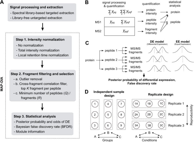
(A) The workflow of data processing and analysis using mapDIA. mapDIA applies data preprocessing steps including normalization and fragment filtering and selection steps, and then performs statistical analysis on the processed fragment-level intensity data. (B) Protein/peptide quantification possibilities using the data extracted from DIA data. DIA data enables both MS1 and MS2 quantification. Fragment-level intensities from MS2 data can be rolled up to peptide-level intensities, which can further summarized into protein-level intensities. Statistical analysis for comparing abundance levels at the protein level can be performed using any of the three types of data: protein, peptide, or fragment-level intensities. The basic architecture of mapDIA was designed to perform protein-level differential expression analysis using fragment-level intensity data. However, simple reformatting of input data allows the user to apply the method to perform the same analysis using peptide or protein-level intensity data. (C) A conceptual diagram of the hierarchical model in mapDIA. Probability models representing differential expression and non-differential expression are estimated for each protein, and the significance score is computed as the posterior probability of the former. The FDR can be directly estimated at each score threshold, facilitating the choice of differentially expressed proteins at the target FDR. (D) Two experimental designs in mapDIA analysis. All pairwise comparisons can be made in a single mapDIA run as requested by the user. Independent sample design offers differential expression analysis between groups of individual samples, whereas replicate design offers within-replicate comparisons over multiple conditions, e.g. time course or dose-dependent experiments replicated in more than one biological replicate. In the Replicate design, reproducible changes in the same direction across multiple replicates lead to greater confidence scores for proteins (or peptides).
Although the TIS normalization procedure is widely used, it is an adjustment by a single normalization factor for all fragments in each sample and therefore it lacks the flexibility to accommodate the systematic variation in TIC differences by the RT. To accommodate local variations in the total ion chromatogram in RT, we developed a local normalization procedure termed RT(δ) normalization. Let T = (t1, …, tF) denote the RTs of all F fragments in the dataset (where RT is defined, e.g., as the apex of the elution peak of each fragment or its precursor). Then the RT(δ) normalization transforms the data as:
| (2) |
where gδ(Δt) is the normal density function evaluated for RT difference Δt with mean 0 and standard deviation δ, and δ is the user-specified RT window for local normalization. Similar to the global TIS normalization, we multiply the normalized data by a constant factor to put the intensities back on a comparable scale as the original data.
In this procedure, it is crucial to ensure the window size δ is not too small since an extremely small window will cause the local normalization factor to be dominated by the intensity of the fragment itself (or other fragments of the same peptide). On the other hand, a large δ will lead to an equivalent outcome to the TIS normalization. In a typical 2–3 hour chromatography gradient, our recommended choice of δ is between 10 and 30 minutes in proteomics applications (experiments with ≥2 hour gradient); the exact value can be decided based on the visualization of total ion chromatograms of all samples on the same panel. The range of 10 to 30 minutes empirically resulted in similar and stable normalization in the datasets we have analyzed so far.
Once the data are normalized, we apply log2 transform to the resulting fragment intensity data and center the log2 intensities for each fragment by the median value across samples. The median centering is performed differently depending on the experimental design (Figure 1A): for each fragment, we compute the median across all the samples for the independent sample design, whereas we compute it within each biological replicate for the replicate design. The reason for computing the median for each biological replicate in the replicate design is as follows: the basal protein abundance is the same within each biological replicate, but not between replicates. The median value(s), computed for each fragment according to the corresponding experimental design, is subtracted from respective fragments. See the experimental design section below for the details of independent sample design and replicate design.
Step 2: Fragment filtering and selection
In the next preprocessing step (Step 2), mapDIA performs a three-tiered fragment filtering and selection procedure (Figure 1A). Exclusion of noisy or irreproducible fragments is critical for statistical analysis because data extraction is typically performed in one sample at a time and thus not all fragments are detected and measured consistently across different samples.
(Step 2a) The first filter detects outlier fragment intensity data (Step 1a). We define outlier fragment intensity as a fragment log2 intensity data substantially deviating from the average median-centered log2 intensity of all other fragments within the same protein. To find these observations, we apply row-wise median centering to the log2 intensity data for all fragments in each protein, compute sample standard deviation of the fragments in each sample, and tag an observation as outlier if its intensity is outside a certain bound (default ±2sd) in the sample. Note that this step removes the fragment intensity data in each sample, not across all samples at once.
(Step 2b) The second filter searches for the most reliable fragments based on the median cross-fragment correlation of quantitative data. Suppose that protein p contains Fp fragments. We first compute the correlation matrix (Fp × Fp) between all pairs of fragments, where the entry in the row a and column b is the Pearson correlation between fragment a (ya) and fragment b (yb). We denote the median correlation of a fragment f by , where the median is taken over the correlations with all other fragments (excluding the self correlation). This median correlation will serve as the consistency score for the given fragment within the parent protein. After score calculation, the fragments with are removed by the user specified threshold m*. As a result of this filter, the fragments that are correlated with the majority of other fragments in each protein will be retained. In addition, the user can specify the maximum number of fragments per peptide (K) to keep the number of available fragments balanced for different peptides, where the top K fragments are selected based on average cross-fragment correlation within each peptide. See examples and guidelines for choosing the optimal parameters in the software user manual.
(Step 2c) The third filter sets inclusion/exclusion criteria based on the minimum number of fragments R and peptides Q available for each protein. Since our model requires repeated measurements for each peptide, at least two fragments must be available per peptide. In our experience so far, there are typically a large number of proteins that will be quantified by a single peptide, and the decision as to whether these proteins should be included or not must be made by the user and specified in the input parameter setting depending on the circumstances. The suggested default threshold values for protein and peptide-level differential expression analysis can be found in the example datasets distributed in the mapDIA package.
Step 3: Statistical model for differential expression analysis
Basic modeling framework: Markov random field model
Using the preprocessed data, mapDIA proceeds to the differential expression analysis based on a Bayesian latent variable model with Markov random field prior, an adaptation of the model described in Wei and Li [15] with application to genomic data analysis. While our implementation automatically performs all pairwise comparisons requested by the user, here we describe the model for a comparison of two groups of samples for the clarity of explanation. The latent variable model can be first written as
| (3) |
where the observed data yp for protein p, including all rows in Y corresponding to the fragments of protein p, is associated with the latent state zp. zp = 1 and zp = 0 indicate that protein p is differentially expressed and non-differentially (equally) expressed, respectively. Denoting the two groups in comparison by i and j,
| (4) |
| (5) |
| (6) |
where π(Θz) denotes the prior distribution of all model parameters for differential expression status z, and denote the peptide index set for protein p and fragment index set for peptide q respectively, and denote the sub-vector of yf and the sub-matrix of yq in the comparison group g respectively. Here φ (·) denotes the product of all element-wise Gaussian densities, i.e.
where fragment f is from peptide q, and in protein p. The priors and closed form expression of for differential and non-differential expression are provided in the Supplementary Information.
Significance scores and FDR
We denote the true (unknown) state by Z* and interpret this as a particular realization of the random vector Z. Our goal is to recover the true state Z* from the observed data Y across all comparisons,
| (7) |
where the joint distribution of Z is approximated by the Markov random field model [16]
| (8) |
with ∂p denoting the set of neighbor proteins of protein p on a previously known network. We call such protein groups “modules” hereafter. Note that, if the module information is not utilized (β = 0), then the entire model will be equivalent to the mixture model treating the latent states as independent binary random variables. From the model above, we can derive the overall optimal solution Z* or derive the posterior probability of differential expression (with no module information) as the final protein significance score for comparing group i and j:
| (9) |
omitting subscripts for the comparison groups i and j. In addition, we provide the posterior odds as a supplemental score (in natural log scale), which is useful when further prioritization is needed among the high scoring proteins (e.g. among the proteins scoring ŝp = 1).
When the module information is utilized, the probability and odds scores are derived in the same manner by using the approximation
| (10) |
| (11) |
Once the scores {ŝp} are computed, the Bayesian FDR [17] is computed as
| (12) |
The details of posterior distributions and estimation procedure can be found in the Supplementary Information.
Experimental designs with independent samples versus replicates
The model derivation above is based on the independent sample comparisons (Figure 1D), where the samples in one group are compared to those in another group. An example of this experimental design is the glycoproteomic data we present later, where 2 or 3 samples from each of 4 different prostate cancer stages are compared in a pairwise manner. In our modeling scheme, the replicate design (Figure 1D) refers to a situation where two or more conditions are compared within each biological replicate and the consistent changes across biological replicates are sought after. An example of replicate design will be shown in the analysis of the dynamic interactome data of 14-3-3β, where the time course expression before and after a certain treatment is monitored within each of three biological replicates of an affinity purified sample. In the analogy of conventional hypothesis testing, the independent sample design corresponds to the t-test for two independent samples, whereas the replicate design corresponds to the t-test for paired samples. mapDIA does not allow nested replicates in the comparisons, i.e. biological or technical replicates for individual samples when the comparison is made between groups of samples.
For modeling the data in the replicate design, a reasonable modification is to derive a similar model with replicate specific mean parameters and use the resulting marginal likelihood in the Markov random field model. However, we discovered that this leads to over-parameterization and usually performs poorly in small sample datasets. For this reason, we remove replicate specific averages (median) from the data prior to modeling and analyze the data using the same model as the independent sample design. This adjustment removes the differences in the baseline intensity levels across different replicates and thus achieves reliable modeling of the data without the over-parameterization problem mentioned above. Note that, unless otherwise stated, replicates should be understood as biological replicates, not technical replicates (repeated MS runs over the same biological specimen), as the variability in such datasets do not represent the biological variation assumed in the variance component of the model.
Simulation data
In the simulation study, we generated log2 intensity data for two group comparison (group A and B) from the following simulation model:
| (13) |
for p = 1,…,1, 500, q = 1,…, np, f = 1,…,npq, and each group had 3 samples. Here xpqj ~ N(0, τ2) and epqfj ~ N(0, σ2)represent the intensity deviation of peptide q from the protein abundance in sample j and measurement error for fragments, respectively. The term x0 corresponds to the effect size (the magnitude of differential expression for the protein) in log2 scale, the set D is the set of differentially expressed proteins, and SB is the index set for samples in group B.
Supplementary Figure 3 illustrates how these two factors affect the simulated data. Panels A through D correspond to (τ, σ) = (0.3, 0.3), (0.1, 0.3), (0.3, 0.2) and (0.1, 0.2). In each panel, the log2 fragment intensities of each peptide were visualised by the dots of the same color, with additional lines connecting them across the samples. First, the parameter τ represents the variability between peptides, in other words, the distance between the lines of different colors in the visualized data. Hence for a fixed value of measurement error σ, a small value of τ reflects high correlation between different peptides (panel B compared to A, panel D compared to C). On the other hand, the parameter σ represents the measurement error of fragment intensities, and this can be interpreted as the distance between lines of the same color within each peptide. Here for a fixed value of peptide deviation τ, a small value of σ reflects high correlation between fragments belonging to the same peptide (panels C/D compared to A/B).
In all simulation scenarios, we generated 100 datasets and averaged the results to produce the pseudo receiver operating characteristic (pROC) and FDR accuracy plots, where pROC is pseudo in the sense that (1-specificity) was replaced by the FDR in the horizontal axis. Specifically, we created 150 differentially expressed proteins and 1,350 background proteins, i.e. 10% of the proteins are differentially expressed in each simulation set. We set the effect size at x0 = 1 (2 fold) and the fragment level variability at σ = 0.2 and σ = 0.3, and varied peptide level variability τ between 0.1 and 0.3. Note that the peptide abundance deviates more from the true protein abundance as τ increases, i.e. quantification of peptides becomes less correlated with the underlying protein abundance level in each sample. In each simulation setup, we mixed proteins containing a different number of peptides and fragments (np, npq) = (2, 3), (2, 5), (5, 5) per protein in equal proportions.
In the simulation with module information, we created the most ideal scenario where the module information can be maximized the most to demonstrate the concept. To do this, we first created a scale-free network (Supplementary Figure 4) using the algorithm of Herrera and Zufiria [18], and verified that the degree of connectivity follows the power law as expected in such a network (P (k) ~ k−2.03). Next we allocated 150 differentially expressed proteins in local subnetworks (see Supplementary Information) so that these proteins are network neighbors with one another. Using one realization of this network generation process, we simulated 100 datasets the same way as above, and compared the performance of mapDIA with and without the network (module) information.
Results
Overview of mapDIA workflow
Our analysis framework follows a three-step workflow (Figure 1A). The input data should be obtained from a signal processing software that extracts peak features, either via targeted extraction of fragment intensities using spectral assay libraries (e.g. OpenSWATH, Skyline) [8, 11] or using DIA-Umpire that allows direct identification of peptides from DIA data without the need for an external spectral library [9]. The input data are further processed in two preprocessing steps by mapDIA, namely intensity normalization (Step 1) and fragment selection (Step 2).
In the first step, mapDIA offers two optional normalization methods. One approach is the widely-used procedure of scaling the data by the total intensity sum in each sample (TIS), which essentially corrects for the variation in the total amount of sample analyzed in a particular run. We also developed an alternative procedure that scales intensity data by the locally weighted intensity sums on the RT axis, which is applied to each fragment in each sample separately. The latter procedure is more adaptive than the TIS-based universal normalization in the sense that temporal fluctuations in the chromatography and measured MS intensities can be adjusted [19].
The next step (Step 2) is fragment filtering and selection. This is a critical step since the data extraction tools process each sample independently, and as a result the detection rate and quantification quality is not the same across all reported peptides and fragments. In mapDIA, there are three-tiered selection thresholds, including (a) standard deviation tolerance to define outliers, (b) minimum average cross-fragment correlation, and finally (c) minimum number of peptides and fragments required for differential expression analysis.
The last step (Step 3) is the model-based analysis for selecting differentially expressed proteins. Although mapDIA’s probability model is constructed flexibly enough to accommodate peptide and protein intensity data (Figure 1B), we will describe the model primarily for the analysis of fragment intensity data. mapDIA embodies a Bayesian hierarchical model for multi-group comparisons, which borrows statistical strength across all proteins in each dataset and thus confers robustness to the significance analysis, especially when the sample size is small (e.g. 3 samples per group). By contrast, the existing software package MSstats fits an independent fixed effects or random effects regression model for each protein and performs statistical significance inference using p-values with multiple testing correction [20], which depends on the accurate estimation of fixed effects parameters and prediction of random effects parameters with a limited number of samples.
The structure of the probability model for individual proteins in mapDIA is illustrated in Figure 1C. After median centering of the log scaled data, each fragment intensity is considered as a repeated measurement of the parent peptide and is modelled by probability distributions under the differential expression (DE model in Figure 1C) scenario and equal expression (EE model) scenario, respectively. The posterior probability and the posterior odds of differential expression are the significance scores for individual proteins and the false discovery rate (FDR) estimates are reported to facilitate the selection of differentially expressed proteins with target FDR [17]. This model is constructed for two common experimental designs, namely independent sample comparison and within-replicate comparison (Figure 1D; See Experimental Procedures for details), adding to the flexibility of our method to various kinds of experimental data.
Simulation study
Key factors in simulation
We performed extensive simulation studies to evaluate the ability of mapDIA to identify differentially expressed proteins. Although data preprocessing steps are essential components of mapDIA, the major goal of this simulation study was to evaluate the performance of the model in comparison to MSstats [14]. The comparison focused on classification of proteins into differentially expressed proteins and non-differentially expressed ones, and on the quality of FDR estimation. We disabled data preprocessing steps in mapDIA so that these steps do not give mapDIA an unfair advantage.
As mentioned in the Introduction, we varied two factors that are likely to affect quantification based on our empirical observation over several test datasets. The first factor is τ, the deviation of peptides from the underlying protein abundance pattern across the samples, i.e. lack of correlation of isolated precursor ions (peptides) with their parent protein. The second factor is σ, the measurement error or noise in the fragment intensities, which can be interpreted as the lack of correlation of the fragments with the abundance of their precursor peptides. Based on our empirical observations, the correlation of fragments with their precursor peptides tended to be better than that of peptides with their precursor proteins. One extra factor we varied was the number of data points per protein, which was controlled by the number of peptides per protein (np) and the number of fragments per peptide (npq). Fixing the values for the first two factors (τ, σ), we would expect that the simulation performance improve as more data are reported per peptide and per protein basis.
Classification performance and FDR accuracy
We generated simulation datasets with different values of these two key parameters that affect the performance of the model (see Experimental Procedures). In all simulation settings, mapDIA and MSstats showed comparable performance (Figures 2A and 2C, Supplementary Figure 5A and 5C). This comparable classification performance was repeated even when the peptide abundance was very inconsistent with the protein abundance (τ = 0.3). The classification performance was more affected by the correlation of peptide-level abundance to the parent protein than the measurement error of fragment intensities (correlation of fragment intensities to their parent peptide). With regard to the data volume, as expected, the classification performance improved as more peptides and fragments were included (data not shown).
Figure 2.
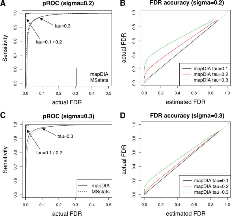
Classification performance and FDR accuracy in simulation studies. In each plot, the measurement error for fragment intensity, denoted by σ, was fixed and the peptide deviation from protein abundance, denoted by τ, was varied. (A, C) Sensitivity versus FDR (pseudo-ROC curve) plot. The actual FDR refers to the average of false discovery proportions over 100 simulations, not the estimated FDR. (B, D) FDR accuracy plot as peptide-level intensity deviates from true protein-level abundance (increasing τ). For each method, τ was varied between 0.1 and 0.3 at a fixed value of σ (0.2 or 0.3).
However, the accuracy in the FDR estimates was markedly different between mapDIA and MSstats (Figures 2B and 2D, Supplementary Figure 5B and 5D). In mapDIA, the FDR estimates were highly accurate when the peptide deviation τ was below 0.2 (data for τ < 0.2 not shown due to overlap), and the FDR began to be underestimated as τ increased above 0.2 (green and red line, Figure 2B and 2D). Consistent with the classification performance, the FDR accuracy was more dependent on the peptide-level correlation to the protein abundance than on fragment intensity correlation to the peptide abundance. For a fixed level of fragment level variability σ = 0.2 or σ = 0.3, the FDR estimates were more heavily underestimated in the critical region (e.g. FDR < 0.1 in Figures 2B and 2D) when peptide-level deviation from protein abundance τ became greater. This suggests that the peptide-level consistency to the parent protein abundance becomes much more influential for the error control in mapDIA when the fragment intensity measurement error is low, i.e. when the peptide deviation dominates the fragment measurement error. It should be noted that the data preprocessing steps of mapDIA, which were not factored into this simulation, were specifically implemented to prevent these scenarios (the filtering Step 2b based on the median cross-fragment correlation score should remove most fragments and peptides with inconsistent quantification from the estimation of the parent protein abundance levels).
In contrast, MSstat had more difficulty with estimating FDR in these data. To avoid suboptimal performance due to incorrectly specified parameters in MSstats, we have evaluated its performance with variable settings. In MSstats, the choice of fixed effects model versus mixed effects model over the biological replicates and/or the MS runs (technical replicates) is a major parameter. Since we assume that each biological sample is analyzed in an independent MS run in our simulation, these are neither biological nor technical replicates as defined in the MSstats package. However, assigning different biological replicate IDs to the samples and assigning identical biological replicate IDs in produced very similar results. At the same time, changing from fixed to random effects in the model (scopeOfBioRep option) affected the outcome dramatically. Including random effects in the model led to highly conservative adjusted p-values, but the default fixed effect model yielded very instable adjusted p-values, and an associated heavy underestimation of the FDR (Supplementary Figures 5B and 5B). This phenomenon prompted us to investigate this behavior carefully in all the real experimental datasets, and this pattern remained consistent in those datasets (also see below).
Simulation study with module information
We also evaluated mapDIA for datasets in which additional module information is available, e.g. relational information between proteins (with the idea that proteins within the same module are likely to co-vary). Modular information can be obtained from protein-protein interaction data (e.g. iRefIndex [21]) or co-annotation of proteins to the same functional category (e.g. Gene Ontology [22] or Reactome [23]). Another example of modular setting is to use peptide-protein membership as the module information when mapDIA is applied to score individual peptides, not proteins (as shown later in the prostate cancer glycopeptide analysis). We generated simulation datasets with differentially expressed proteins spatially positioned in network modules (see Experimental Procedures). As expected, simulation results suggest that mapDIA assisted with the module information through the Markov random field prior brought significant improvement in the classification performance and FDR accuracy (Supplementary Figure 6). The improvement was pronounced for proteins that had only a few peptides and fragments, specifically for proteins with 2 peptides and 3 fragments per peptide. Nevertheless, there are two caveats here. First, our analysis was conducted assuming that we have the complete knowledge of the underlying network/module. Second, the differentially expressed proteins are often dispersed throughout the entire network in realistic datasets, i.e. not as concentrated around a subnetwork as in our simulation example. Both properties are not likely to be satisfied in real applications, and therefore the performance improvement will likely be more moderate than in our demonstration. However, such module information is still useful in real setting, as we later demonstrate in the analysis of glycoproteomics data.
Analysis of 14-3-3β dynamic interactome data
We applied mapDIA to a recently published SWATH-MS dataset by Collins et al [24], who investigated the 14-3-3β interactome in IGF-stimulated HEK293 cells via affinity purification-mass spectrometry (AP-MS) experiments in a time-resolved manner. The AP-MS experiments were performed in three biological replicates at six time points: the PI3K inhibitor LY294002 was added to prevent AKT activation (−60 minute) prior to IGF1 stimulation (0 minute), and the interactome was followed at four post-treatment time points (1, 10, 30, and 100 minutes) after IGF1 stimulation. GFP control purifications were also prepared in triplicates at each of three time points (−60, 0, and 30) to remove non-specific binders. The SWATH-MS data was extracted using OpenSWATH by targeted extraction using an existing spectral assay library as described in [24], which produced the original data for 1,967 proteins, 16,180 peptides, and 85,545 fragments across all bait and control purifications.
We performed the data analysis similar to the original paper, and used mapDIA (replicate design, Figure 1D) and MSstats for downstream analysis. Since AP-MS experiments capture contaminants in addition to real interaction partners [25, 26, 27], we first compared the bait purification to the control purification at each of the three time points using mapDIA, and identified 648 proteins significantly enriched in the bait purification over controls (1% FDR) at one or more time points. This step reduced the number of peptides and fragments to 8,309 and 43,575, respectively. Using this contaminant-filtered data, we performed the differential expression analysis to detect protein abundance changes at each time point against the baseline at IGF1 stimulation (0 minute) using mapDIA and MSstats.
Fragment filtering and selection
Throughout the analysis, we applied 2 standard deviation threshold for outlier detection, median cross-fragment correlation 0.2 with a maximum number of fragment per peptide K = 5, and at least 1 peptide per protein/3 fragments per peptide in the fragment selection step (see Experimental Procedures for details). Since normalization of quantitative data in dynamic conditions can remove real biological signals [28], we applied no normalization procedure to this dataset. Figure 3A shows the outlier detection and removal step in the time course analysis, where the green boxes indicate the outliers that are removed in specific samples. Following this step, for each fragment, the Pearson correlation was computed with all other fragments within the same protein and the median cross-fragment correlation was reported as the consistency score for that fragment. The fragments with median cross-fragment correlation score below the threshold (0.2) were removed from further analysis (Figure 3B–3C). Finally, mapDIA analyzed the proteins containing at least Q peptides each with at least R fragments for statistical analysis (with Q and R specified by the user, see below).
Figure 3.
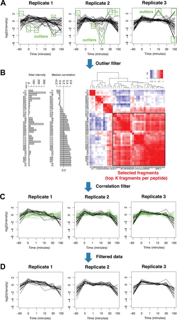
(A) The extracted fragment intensity data for a sample protein in the 14-3-3β dataset. Each black line is the time course trajectory of fragment intensity data in each biological replicate. The first step detects outliers at each time point within each replicate. Green boxes indicate the log2 intensity values that are 2 standard deviation away from the mean at each time point. The data shown are after log2 transformation and centering within each replicate under the Replicate design. (B) After outlier removal, the median cross-fragment correlation is used to score the reliability of each fragment. The dashed line 0.2 is a user-specified correlation threshold, and the fragments with the median correlation score above this threshold are selected for the statistical analysis. If there are more than the user specified maximum number of fragments per peptide (K), then K fragments with the highest median correlation scores will be selected. (C) The threshold 0.2 leads to removal of the fragments shown in green lines. After removal of the fragments, if the protein still retains at least Q peptides with minimum R fragments in each, the protein is kept for further analysis. (D) The final fragment-level intensity data after all data preprocessing steps are applied.
After this three-tiered filtering and selection step, outlier observations for 4,025 fragments were removed in at least one of the 18 samples (3 replicates, 6 time points), and 8,277 fragments (19%) from 495 of 648 proteins were removed as quantitatively unreliable fragments for the analysis. Lastly, 4,232 fragments were further removed by requiring Q = 1, R = 3 and K = 5, which resulted in the final dataset consisting of 31,038 fragments, 6,872 peptides in 632 proteins. Note that mapDIA reports which filtering step(s) removed each fragment in a separate output file so that the user can tune the filtering criteria in subsequent analyses.
Differential expression analysis in the replicate design
Following the fragment selection step, we ran the differential expression analysis using map-DIA, comparing pre- and post-treatment time points (−60,1,10,30,100 min) against the time at IGF1 stimulation (0 min). Note that quantitative comparison is made at each of the 5 time points for 632 proteins (3,151 comparisons in total; Supplementary Table 1). In mapDIA, the estimated probability score associated with the estimated 1% FDR was s* = 0.825 (no module information), and this threshold gave 1,018 significant comparisons. Here differentially expressed protein refers to a protein that was affinity captured at different concentration levels against 0 minute in at least one of the five comparisons.
Figure 4A shows the plot of the significance scores (posterior probability) against log2 fold change for all five time points of comparison, showing clear separation between significant and non-significant comparisons. Here many proteins with absolute log2 fold change around 0.5 or below (fold change 30% increase or decrease) scored near zero probability. However, there was an increasing tendency to score favorably as the number of peptides and fragments per protein increases, and the distinction between differentially and non-differentially expressed proteins became clear with increasing amount of data per protein. For example, the classification calls were very clear cut once the number of fragments per protein reached 30 or so (1,370 comparisons for proteins with ≥30 fragments). We note that some comparisons were called significant at the target FDR level even with moderate average log2 fold change. These cases came from the proteins in which clear differential expression was observed in two biological replicates across many fragments, but not in third replicate. In the replicate design, mapDIA automatically reports the inter-replicate correlation for each fragment, with which the user can identify these patterns in the final report.
Figure 4.
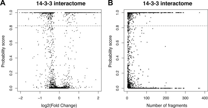
(A) Posterior probability scores for all comparisons plotted against log2 fold change in the 14-3-3β interactome data. Different proteins with similar fold changes may get drastically different confidence scores depending on the reproducibility of fragment-level intensity data and the number of peptides/fragments available for each protein. (B) Posterior probability scores for all comparisons plotted against the number of fragments in each protein in the two methods in the 14-3-3β interactome data. The confidence scores in mapDIA tended to be mildly favorable to the proteins with more peptides and fragments.
Comparison with MSstats
In order to compare the results with MSstats, we again ran the analysis with all possible combinations of fixed effects and random effects terms for both biological replicates and technical replicates, which gave us four different analysis outputs. Consistent with our experience in the simulation datasets, MSstats produced two very different results in terms of the reported p-values dependent on the fixed vs. random effects option selected (Supplementary Table 1). When random effects were specified for biological replicates, merely 127 comparisons were found to be significant at 1% FDR threshold, whereas 2,244 comparisons (out of 3,151) were reported to be significant when fixed effects were specified (Supplementary Figure 7A). The options for technical replicates made minor differences only.
When fixed effects for biological replicates were used for comparison in MSstats, the statistically significant comparisons from mapDIA were completely nested within the selection by MSstats (1,008/1,018), even though the two algorithms reported almost perfectly correlated log2 fold changes (Supplementary Figure 7B). We compared the fold change distribution and the inter-replicate reproducibility of the proteins called significant by both mapDIA and MStats and those only identified as significant by MStats. Proteins identified by MStats alone tended to exhibit more moderate fold changes (the fold change in the majority of these proteins was 40% or less; Supplementary Figure 7C). When we examined the relationship between the p-values and the number of peptides and fragments, the majority of comparisons (1,154) in those proteins with ≥30 fragments (1,370) were called statistically significant by MSstats in the data with fixed effects for biological replicates (Supplementary Figure 7D). Taken together, this suggests that the additional comparisons reported as significant by MSstats tended to come from the pool of proteins with a large number of fragments showing only moderate fold changes. The comparisons called significant in MSstats also tended to come from the proteins with lower inter-replicate correlations (Supplementary Figure 7E).
We further analyzed the enrichment of Akt substrates (Akt1/Akt2) in the top scoring comparisons made by MStats alone and MStats/mapDIA. Akt is the central kinase in the insulin-IGF1 signalling pathway modulated by the perturbation, and substrates of Akt are well known to bind 14-3-3 proteins at the phosphorylated site. As such, binding of Akt substrates to 14-3-3 is expected to be significantly modulated by this treatment. The substrate list was extracted from PhosphoSitePlus [29] and NetworKIN [30] and the comparisons were ordered by the log odds scores for mapDIA and adjusted p-values for MSstats. Supplementary Figure 7F clearly shows that Akt substrates were more enriched in the comparisons prioritized by mapDIA than that by MSstats. Therefore, while mapDIA produces a smaller list of significantly changed proteins than MStats, mapDIA does not appear to be underpowered, and is capable of revealing likely biologically meaningful changes.
Analysis of prostate cancer glycoproteomics data
We next re-analyzed a published glycoproteomics dataset of prostate cancer samples with varying tumor aggressiveness [31]. In this study, N-linked glycopeptides were isolated from 10 normal (N), 24 non-aggressive (NAG), 16 aggressive (AG) and 25 metastatic (M) prostate cancer samples, and each group was pooled into 2 or 3 sample pools and analyzed by SWATH-MS (effective samples sizes are 2 N, 2 NAG, 3 AG, 3 M). We first extracted the data for 302 glycoproteins (2,641 peptides, 27,361 fragments) using the recently developed DIA-Umpire tool [9]. Note that the DIA-Umpire pipeline includes an optional user-selected fragment/peptide selection module applied prior to computing protein-level protein intensities. In this analysis, we disabled the selection module and used the entire set of fragment intensities extracted by DIA-Umpire (i.e. not subject to DIA-Umpire’s fragment/peptide selection procedure). Using this data, we performed peptide-level differential expression analysis using mapDIA in the independent sample design (Figure 1D) for all 6 pairwise comparisons (between the four groups). In mapDIA, the analysis can be performed at the peptide-level by specifying the peptide identifier as the protein name in the input data.
Intensity normalization
In this dataset, we first tested all variants of intensity normalization methods implemented in mapDIA. According to a recent report that investigated the variation in multi-center pro-teomic data [19], the major sources of systematic variation included the chromatographic retention time (RT) and ion suppression during the ionization in each MS run. The temporal variation can be addressed in mapDIA using the RT(δ) normalization (see Methods). Here we used Gaussian kernel weights with standard deviation of δ = 10 and δ = 30 min utes to compute the normalization factor locally for each fragment, with weights assigned to the adjacent fragments in the m/z and RT axes. If there is no such temporal or local variation, then this normalization method should produce similar results as the TIS normalization where all fragment intensities are divided by the total fragment intensities in each sample. When we compared the results obtained using no normalization, TIS-normalization, and RT(10) and RT(30) normalization, the fragment intensity data were significantly more correlated in RT(10) normalized data between samples belonging to the comparison group (Supplementary Figure 8), indirectly suggesting improved normalization of the data therein. We therefore decided to use the RT(10) normalized data for further downstream analysis (see Supplementary Figure 9 for the TIC profiles across the 10 samples before and after normalization).
Peptide differential expression analysis in the independent sample design
We performed peptide differential expression analysis using mapDIA under the independent sample design (Figure 1D) and MSstats, comparing every pair of groups (up to 6 comparisons per protein). We noticed that MSstats reported significance scores for 12,174 comparisons whereas mapDIA reported scores for 6,735 comparisons, where mapDIA removed a large number of comparisons due to minimal fragment requirement (Q, R) = (1, 3) (Supplementary Table 2). Therefore we compared the two methods only for the comparisons reported from both (6,735 in total).
At the 1% FDR threshold in each method, mapDIA and MSstats reported 2,083 and 4,869 comparisons as significant, respectively, and the comparisons reported as significant by mapDIA were again almost completely nested within those reported by MSstats. For MSstats, the aberrant behavior of p-values were observed again with the choice of fixed effects and random effects specification in the model. With random effects model, nearly no comparisons were reported to be significant, whereas 72% of the comparisons (4,869/6,735) were found to be significant with the fixed effects model (Supplementary Figure 10). Since the random effects model of MSstats gave too few significant comparisons, we used the fixed effects model for comparison.
In the mapDIA analysis, statistically significant glycopeptides showed at least a 40% or more of fold change (Figures 5A). Unlike the previous protein-level analysis in the 14-3-3β dataset, this plot looks similar to a typical “volcano plot” one would expect from the analysis of a typical gene or protein expression dataset where each gene or protein is quantified with a single value. This was expected because the analysis was performed at the peptide level, each containing at most 5 representative fragments in terms of cross-fragment correlation, and therefore the amount of data for each unit was much more balanced for peptide-level analysis than for protein-level analysis (e.g. 14-3-3β data).
Figure 5.
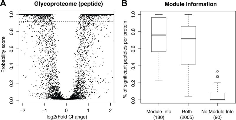
(A) Posterior probability scores for all comparisons plotted against log2 fold change of glycopep-tides in the prostate cancer glycoproteome data (no module information was used). (B) The boxplots of score distributions for the peptides-level analysis. Peptides originating from the same proteins were assumed as the modules, and this module information was utilized in the model fit. This leads to two model fits for peptide-level analysis, with or without module information. Boxplots were drawn separately for the peptides that are common in both analyses and those that are unique to each analysis. The plots show that more glycopeptides were called significant with higher score in the analysis using the module information if their co-member glycopeptides were differentially expressed.
Examining the 2,083 significant cases, the majority of these comparisons came between cancer patients and controls (transplant donors) and between the MET group and AG/NAG groups. When we examined the estimated fold changes reported from both methods, they were again highly correlated (r = 0.99, Supplementary Figure 11). This indicated that the difference in the significant comparisons at the same FDR threshold is due to the differences in the statistical approaches applied to model the variability in the data, and not from the estimation of effect size (magnitude of change).
Analysis using the module information
In certain experimental designs, co-variation of proteins or peptides may be expected: in these cases, allowing an experimental design that makes use of such information may be beneficial. We refer to these associations as modules, and in its current implementation, mapDIA can use protein interaction or other annotation data as a source of modules, but in the case of inference at the level of peptides, it can also use the parent protein as a module. Hence, here we also tested the mapDIA performance at the peptide level for the glycopeptide data, by specifying peptide names as the protein identifiers in the mapDIA. In this dataset, this specification essentially represents the hypothesis that a glycopeptide is more likely to be differentially expressed if other glycopeptides in the same protein are also differentially expressed. If this hypothesis holds true, then the Markov random field model will effectively utilize such information. Otherwise, then the model will automatically downplay such associations and differential expression status will be inferred independently for each peptide.
When the module information was utilized through the Markov random field model (see Methods), 2,173 comparisons were found to be significant. The majority of them (1,990) were in agreement between the two models (Supplementary Table 3). As expected, additional differentially expressed peptides in the model with the module information were found to belong to the proteins containing other peptides reported as differentially expressed. Figure 5B shows that, when we looked at the 183 additional comparisons significant in the model with module information, on average 75% of the other peptides in the same proteins were significantly differentially expressed peptides. This indicates that the Markov random fields model effectively pooled information within the modules (individual proteins) to boost probability scores for glycopeptides when other glycopeptides in the same protein were differentially expressed and vice versa.
Discussion
In this work, we presented a novel software package, mapDIA, for statistical analysis of quantitative proteomics data generated in the DIA mode. Our data preprocessing routines include normalization methods that can remove systematic bias that is constant or temporal between MS runs, and a series of fragment filtering and selection procedures to remove outlier observations and irreproducible fragments. The statistical model had previously been developed for microarray data [15] and here we modified the same modeling framework to account for the protein-peptide-fragment hierarchy in DIA data. As we illustrated in both simulation and real experimental DIA data, mapDIA yields sensitive selection of differentially expressed proteins and allows robust control of the FDR. Unlike most other methods previously applied to DIA data, mapDIA explicitly utilizes repeated measurements (multiple fragments/peptides) of the protein abundance, which is a unique feature of MS2 fragment-level quantification offered by the DIA-MS. The software is also flexible enough to accommodate different experimental designs, and allows robust estimation of the FDR even in datasets with a small number of samples.
We have used MSstats as our main benchmark for comparison in this work. Importantly, our motivation was not to highlight the potential deficiencies of MSstats - a valuable tool for SRM/MRM based quantitative data - but to better understand the challenges presented by the more complex DIA-MS data. The conclusion we drew in the performance comparison warrants further investigation across a larger number of datasets. It is likely that the main reason behind the suboptimal performance of MSstats observed in this work is related to the inherent differences between the SRM/MRM and the DIA-MS data. In SRM/MRM, for which MSstats was developed, the protein-peptide-transition pairing is carefully selected, which yields more reliable quantification for protein-level statistical inference. In contrast, DIA-MS data is more complex and inherently noisier (i.e. it contains a larger number of inaccurately quantified fragment ions), and peptide ions isolated in different SWATH windows across the DIA-MS experiment can deviate quite significantly from the average cross-peptide pattern of each protein. As a result, a regression model that handles sample-to-sample variation only at the protein level through fixed or random effects, even in the presence of the interaction terms in their model, may not be sufficient to account for such variability.
The three-tiered fragment selection step is a very important feature of mapDIA. In particular, the median cross-fragment correlation score can effectively remove noisy fragments in both datasets analyzed in this work. These steps are critical because the fragments peak data is extracted in each sample separately and thus the fragment intensity data may not be of the same quality across different samples. Moreover, even with the well behaving fragments, we noticed that a certain degree of data reduction is crucial for reliable statistical modeling in both methods because the amount of data can be severely unbalanced for different proteins, i.e. while some proteins have hundreds of fragments from tens of peptides, others may have a single peptide with only a few reliable fragments. To address this problem, we have allowed the users of mapDIA to control the maximum number of fragments (K) per peptide, where the most representative K fragments in terms of the median cross-fragment correlation score are chosen within each peptide. However, we also remark that excessive application of these filtering steps can lead to spurious findings, and thus our recommendation is to carefully specify the input parameters in a way that the final selection of reliable fragments preserves the underlying quantitative trends across the samples. To facilitate this monitoring process, our software automatically reports the filtering outcome at every stage as a part of the analysis output and also saves the filtered data to allow the users to visualize the data and monitor the changes as different filtering criteria are applied.
With regard to the statistical inference of differential expression, we formulated a hierarchical Bayesian model with the Markov random fields prior, which enables module-oriented analysis. We discovered that this additional feature of prior was impactful when there are a limited number of quantitative data per protein (i.e. a small number of peptides and fragments) as illustrated in our simulation study. For many proteins DIA-MS data provides a sufficient number of repeated measurements (fragments and peptides) to support solid probabilistic decision for protein-level analysis without the need for additional priors in the model. Nevertheless, the model was found to be useful when the number of observations per unit of analysis was relatively small, which occurs in two practical scenarios. First, when the quantitative data is rolled up to the protein or peptide level (summed over fragments and peptides), the model can incorporate the functional module information such as Gene Ontology and protein-protein interaction data in the differential expression analysis, assuming that the proteins in a common functional module are likely to behave similarly. Second, as we demonstrated in the glycoproteomic data, the model can be used for peptide-level analysis using the protein identifiers as the modules. mapDIA’s data input format was flexibly designed to accommodate various types of module information (see our software manual).
A frequently arising topic in the statistical analysis of label-free quantitative data is the treatment of missing data. Currently, we do not perform any missing data imputation or model-based treatment in mapDIA. We analyze the data using fragments with non-missing data in at least two samples within each comparison group in the independent sample design, or using fragments with no missing data in the replicate design. While the existing missing data imputation methods such as the nearest neighbor-based approach are appealing, their performance has not been benchmarked using gold standard DIA datasets. More fundamentally, it is difficult to judge whether such methods represent the underlying mechanism resulting in missing data in DIA experiments, which is non-random and associated with various components of the data extraction pipelines (e.g. de-convolution of co-eluting ions, data extraction parameters, the quality of DDA spectral library in targeted extraction, etc.). Indeed, the missing data problem can potentially be better addressed at the data extraction stage, where one can further reduce the number of missing values via improved algorithms for detection and quantification of low abundance fragment ions at the limit of detection.
Finally, the current implementation of mapDIA requires that fragment intensity data be organized in the two-layered hierarchy, that is, protein to peptides and peptides to fragments. However, the software can be immediately applied to protein intensity and peptide intensity datasets. As mentioned earlier, for example, quantitative phosphoproteomics analysis requires significance scores at the peptide level, and the user can format the data with peptide sequences as protein and peptide identifiers, which will inform the software to compute scores for peptides. Likewise, protein-level analysis can be performed if protein intensities are provided along with protein ID specified as protein/peptide/fragment identifiers.
Overall, we believe that mapDIA enables robust statistical analysis of DIA quantitative proteomics data. Refinements are planned and will be introduced in the future releases of mapDIA, such as handling of technical/biological replicates in the independent sample design, additional options to adjust the stringency of fragment selection steps, and more elaborate evaluation of the built-in normalization methods. More importantly, a comprehensive investigation of the interplay between various data extraction methods and the preprocessing steps in mapDIA will be of utmost interest, which will reveal the optimal integrated data analysis pipeline for this type of data from start to finish.
Supplementary Material
Significance of our work.
Data independent acquisition mode of mass spectrometry (DIA-MS) is an emerging topic in the quantitative proteomics literature. While currently published reports are primarily focused on the DIA instrumentation and data extraction methods, our manuscript presents one of the first statistical tools, called mapDIA, to perform rigorous data preprocessing in the context of multi-sample DIA data and robust statistical analysis to determine differential expression status using DIA data. mapDIA also features a flexible intensity normalization procedure and an advanced probabilistic model that can incorporate biological networks in the detection of differentially expressed proteins.
Highlights.
We developed mapDIA, one of the first statistical methods for differential protein expression using the data produced from data independent acquisition mass spectrometry.
mapDIA provides an interactive user interface to filter out outliers and poorly quantitated fragment-level intensity data, commonly found in DIA-MS data produced by the library-based or library-free data extraction step.
mapDIA also offers a flexible retention time-based normalization method.
The core of mapDIA consists of the Bayesian hierarchical model for differential expression analysis, which yields a highly sensitive scoring system with good control of false discovery rates.
The model can also incorporate biological network data through the Markov random field model, which tends to detect differentially expressed proteins in relevant sub-networks.
The statistical model is applicable to two commonly used experimental designs, namely comparison of independent biological samples and comparison of different conditions within biological replicates (e.g. time course).
Acknowledgments
This work was supported in part by a grant from the Singapore Ministry of Education (to HC; R-608-000-088-112), the US National Institutes of Health (to A.I.N and A.-C.G; 5R01GM94231), the Canadian Cancer Society Research Institute through an Innovation grant (to A.-C.G.) and the Government of Canada through a Genome Canada Genomics Innovation Network and Canadian Institutes of Health Research grants (to A.-C.G.). We are grateful to Christine Vogel for helpful discussion, and Jean-Phillippe Lambert, Brett Larsen, and members of the Aebersold lab for providing the test datasets and testing the mapDIA software.
Abbreviations
- AP-MS
Affinity Purification - Mass Spectrometry
- DDA
Data Dependent Acquisition
- DIA
Data Independent Acquisition
- FDR
False Discovery Rate
- pROC
pseudo Receiver Operating Characteristic
- RT
Retention Time
- TIC
Total Ion Chromatogram
- TIS
Total Intensity Sum
Footnotes
Publisher's Disclaimer: This is a PDF file of an unedited manuscript that has been accepted for publication. As a service to our customers we are providing this early version of the manuscript. The manuscript will undergo copyediting, typesetting, and review of the resulting proof before it is published in its final citable form. Please note that during the production process errors may be discovered which could affect the content, and all legal disclaimers that apply to the journal pertain.
Availability: The software was written in C++ language and the source code is available for free through SourceForge website http://sourceforge.net/projects/mapdia/.
References
- 1.Michalski A, Cox J, Mann M. More than 100,000 detectable peptide species elute in single shotgun proteomics runs but the majority is inaccessible to data-dependent LC-MS/MS. J Proteome Res. 2011;10(4):1785–1793. doi: 10.1021/pr101060v. [DOI] [PubMed] [Google Scholar]
- 2.Gillet LC, Navarro P, Tate S, Röst HL, Selevsek N, Reiter L, Bonner R, Aebersold R. Targeted data extraction of the MS/MS spectra generated by data-independent acquisition: a new concept for consistent and accurate proteome analaysis. Mol Cell Proteomics. 2012;11(6):O111.016717. doi: 10.1074/mcp.O111.016717. [DOI] [PMC free article] [PubMed] [Google Scholar]
- 3.Venable JD, Dong MQ, Wohlschlegel J, Dillin A, Yates JR. Automated approach for quantitative analysis of complex peptide mixtures from tandem mass spectra. Nat Methods. 2004;1(1):39–45. doi: 10.1038/nmeth705. [DOI] [PubMed] [Google Scholar]
- 4.Carvalho PC, Han X, Xu T, Cociorva D, Carvalho Mda G, Barbosa VC, Yates JR., 3rd XDIA: improving on the label-free data-independent analysis. Bioinformatics. 2010;26(6):847–8. doi: 10.1093/bioinformatics/btq031. [DOI] [PMC free article] [PubMed] [Google Scholar]
- 5.Panchaud A, Scherl A, Shaffer SA, von Haller PD, Kulasekara HD, Miller SI, Goodlett DR. PAcIFIC: how to dive deeper into the proteomics ocean. Anal Chem. 2009;81(15):6481–6488. doi: 10.1021/ac900888s. [DOI] [PMC free article] [PubMed] [Google Scholar]
- 6.Egertson JD, Kuehn A, Merrihew GE, Bateman NW, MacLean BX, Ting YS, Canterbury JD, Marsh DM, Kellmann M, Zabrouskov V, Wu CC, Mac-Coss MJ. Multiplexed MS/MS for improved data-independent acquisition. Nat Methods. 2013;10:744–746. doi: 10.1038/nmeth.2528. [DOI] [PMC free article] [PubMed] [Google Scholar]
- 7.Canterbury JD, Merrihew GE, MacCoss MJ, Goodlett DR, Shaffer SA. Comparison of data acquisition strategies on quadrupole ion trap instrumentation for shotgun proteomics. J Am Statist Assoc. 2014;25:2048–2059. doi: 10.1007/s13361-014-0981-1. [DOI] [PMC free article] [PubMed] [Google Scholar]
- 8.Röst HL, Rosenberger G, Navarro P, Gillet L, Miladinović SM, Schubert OT, Wolski W, Collins BC, Malmström J, Malmström L, Aebersold R. Openswath enables automated, targeted analysis of data-independent acquisition MS data. Nat Biotechnol. 2014 Mar;32(3):219–223. doi: 10.1038/nbt.2841. [DOI] [PubMed] [Google Scholar]
- 9.Tsou CC, Avtonomov D, Larsen B, Tucholska M, Choi H, Gingras AC, Nesvizhskii AI. DIA-Umpire: comprehensive computational framework for data independent acquisition proteomics. Nat Methods. 2015;12(3):258–264. doi: 10.1038/nmeth.3255. [DOI] [PMC free article] [PubMed] [Google Scholar]
- 10.Guo T, Kouvonen P, Koh CC, Gillet LC, Wolski W, Röst HL, Rosenberger G, Collins BC, Blum LC, Gillessen S, Joerger M, Jocum W, Aebersold R. Rapid mass spectrometric conversion of tissue biopsy samples into permanent quantitative digital proteome maps. Nat Med. 2015;21(4):407–413. doi: 10.1038/nm.3807. [DOI] [PMC free article] [PubMed] [Google Scholar]
- 11.MacLean BX, Tomazela DM, Shulman N, Chambers M, Finney GL, Frewen B, Kern R, Tabb DL, Liebler DC, MacCoss MJ. Skyline: an open source document editor for creating and analyzing targeted proteomics experiments. Bioinformatics. 2010;26(7):966–968. doi: 10.1093/bioinformatics/btq054. [DOI] [PMC free article] [PubMed] [Google Scholar]
- 12.Polpitiya AD, Qian WJ, Jaitly N, Petuk VA, Adkins JN, Camp DG, 2nd, Anderson GA, Smith RD. DAnTE: a statistical tool for quantitative analysis of -omics data. Bioinformatics. 2008;24(13):1556–1558. doi: 10.1093/bioinformatics/btn217. [DOI] [PMC free article] [PubMed] [Google Scholar]
- 13.Cox J, Mann M. MaxQuant enables high peptide identification rates, individualized p.p.b.-range mass accuracies and proteome-wide protein quantification. Nat Biotechnol. 2008;26:1367–1372. doi: 10.1038/nbt.1511. [DOI] [PubMed] [Google Scholar]
- 14.Choi M, Chang CY, Clough T, Broudy D, Killeen T, MacLean BX, Vitek O. MSstats: an R package for statistical analysis of quantitative mass spectrometry-based proteomic experiments. Bioinformatics. 2014;30(17):2524–2526. doi: 10.1093/bioinformatics/btu305. [DOI] [PubMed] [Google Scholar]
- 15.Wei Z, Li H. A Markov random field model for network-based analysis of genomic data. Bioinformatics. 2007;23(12):1537–1544. doi: 10.1093/bioinformatics/btm129. [DOI] [PubMed] [Google Scholar]
- 16.Besag J. On the statistical analysis of dirty pictures. J Royal Statist Soc B. 1986;48:259–302. [Google Scholar]
- 17.Newton MA, Noueiry A, Sarkar D, Ahlquist P. Detecting differential gene expression with a semiparametric hierarchical mixture method. Biostatistics. 2004;5(2):155–176. doi: 10.1093/biostatistics/5.2.155. [DOI] [PubMed] [Google Scholar]
- 18.Herrera C, Zufiria PJ. Generating scale-free networks with adjustable clustering coefficient via random walks. arXiv. 2011:1105.3447. [Google Scholar]
- 19.Rudnick PA, Wang X, Yan X, Sedransk N, Stein SE. Improved normalization of systematic biases affecting ion current measurements in label-free proteomics data. Mol Cell Proteomics. 2014;13(5):1341–1351. doi: 10.1074/mcp.M113.030593. [DOI] [PMC free article] [PubMed] [Google Scholar]
- 20.Benjamini Y, Hochberg Y. Controlling the false discovery rate: a practical and powerful approach to multiple testing. J Royal Statist Soc B. 1995;57(1):289–300. [Google Scholar]
- 21.Razick S, Magklaras G, Donaldson IM. iRefIndex: a consolidated protein interaction database with provenance. BMC Bioinformatics. 2008;9:405. doi: 10.1186/1471-2105-9-405. [DOI] [PMC free article] [PubMed] [Google Scholar]
- 22.Ashburner M, Ball CA, Blake JA, Botstein D, Butler H, Cherry JM, Davis AP, Dolinski K, Dwight SS, Eppig JT, Harris MA, Hill DP, Issel-Tarver L, Kasarski A, Lewis S, Matese JC, Richardson JE, Ringwald M, Rubin GM, Sherlock G. Gene Ontology: tool for the unification of biology. Nat Genet. 2000;25:25–29. doi: 10.1038/75556. [DOI] [PMC free article] [PubMed] [Google Scholar]
- 23.Croft D, O’Kelly G, Wu G, Haw R, Gillespie M, Matthews L, Caudy M, Gara-pati P, Gopinath G, Jassal B, Jupe S, Kalatskaya I, Mahaja S, May B, Ndegwa N, Schmidt E, Shamovsky V, Yung C, Birney E, Hermjakob H, D’Eustachio P, Stein L. Reactome: a database of reactions, pathways and biological processes. Nucleic Acids Res. 2011;39:D691–697. doi: 10.1093/nar/gkq1018. [DOI] [PMC free article] [PubMed] [Google Scholar]
- 24.Collins BC, Gillet LC, Rosenberger G, Röst HL, Vichalkovski A, Gstaiger M, Aebersold R. Quantifying protein interaction dynamics by SWATH mass spectrometry: application to the 14-3-3 system. Nat Methods. 2013;10(12):1246–1253. doi: 10.1038/nmeth.2703. [DOI] [PubMed] [Google Scholar]
- 25.Chen GI, Gingras AC. Affinity-purification mass spectrometry (AP-MS) of serine/threonine phosphatases. Methods. 2007;42(3):298–305. doi: 10.1016/j.ymeth.2007.02.018. [DOI] [PubMed] [Google Scholar]
- 26.Gingras AC, Gstaiger M, Raught B, Aebersold R. Analysis of protein complexes using mass spectrometry. Nat Rev Mol Cell Biol. 2007;8(8):645–654. doi: 10.1038/nrm2208. [DOI] [PubMed] [Google Scholar]
- 27.Dunham WH, Mullin M, Gingras CA. Affinity-purification coupled to mass spectrometry: basic principles and strategies. Proteomics. 2012;12(10):1576–1590. doi: 10.1002/pmic.201100523. [DOI] [PubMed] [Google Scholar]
- 28.Loven J, Orlando DA, Sigova AA, Lin CY, Rahl PB, Burge CB, Levens DL, Lee TI, Young RA. Revisiting global gene expression analysis. Cell. 2012;151(3):476–482. doi: 10.1016/j.cell.2012.10.012. [DOI] [PMC free article] [PubMed] [Google Scholar]
- 29.Hornbeck PV, Kornhauser JM, Tkachev S, Zhang B, Skrzypek E, Murray B, Latham V, Sullivan M. PhosphoSitePlus: a comprehensive resource for investigating the structure and function of experimentally determined post-translational modifications in man and mouse. Nucleic Acids Res. 2012;40:D261–270. doi: 10.1093/nar/gkr1122. [DOI] [PMC free article] [PubMed] [Google Scholar]
- 30.Linding R, Jensen LJ, Ostheimer GJ, van Vugt MATM, Jorgensen C, Miron IM, Diella F, Colwill K, Taylor L, Elder K, Metalnikov P, Nguyen V, Pasculescu A, Jin J, Park JG, Samson LD, Woodgett JR, Russell RB, Bork P, Yaffe MB, Pawson T. Systematic discovery of in vivo phosphorylation networks. Cell. 2007;129:1415–1426. doi: 10.1016/j.cell.2007.05.052. [DOI] [PMC free article] [PubMed] [Google Scholar]
- 31.Liu Y, Chen J, Sethi A, Li QK, Chen L, Collins BC, Gillet LC, Wollscheid B, Zhang H, Aebersold R. Glycoproteomic analysis of prostate cancer tissues by SWATH mass spectrometry discovery N-acylethanolamine acid amidase and protein tyrosine kinase 7 as signatures for tumor aggressiveness. Mol Cell Proteomics. 2014;13(7):1753–1768. doi: 10.1074/mcp.M114.038273. [DOI] [PMC free article] [PubMed] [Google Scholar]
Associated Data
This section collects any data citations, data availability statements, or supplementary materials included in this article.