

Abstract
Functional connectivity analysis of the human brain is an active area in fMRI research. It focuses on identifying meaningful brain networks that have coherent activity either during a task or in the resting state. These networks are generally identified either as collections of voxels whose time series correlate strongly with a pre-selected region or voxel, or using data-driven methodologies such as independent component analysis (ICA) that compute sets of maximally spatially independent voxel weightings (component spatial maps (SMs)), each associated with a single time course (TC). Studies have shown that regardless of the way these networks are defined, the activity coherence among them has a dynamic nature which is hard to estimate with global coherence analysis such as correlation or mutual information. Sliding window analyses in which functional network connectivity (FNC) is estimated separately at each time window is one of the more widely employed approaches to studying the dynamic nature of functional network connectivity (dFNC). Observed FNC patterns are summarized and replaced with a smaller set of prototype connectivity patterns (“states” or “components”), and then a dynamical analysis is applied to the resulting sequences of prototype states.
In this work we are looking for a small set of connectivity patterns whose weighted contributions to the dynamically changing dFNCs are independent of each other in time. We discuss our motivation for this work and how it differs from existing approaches. Also, in a group analysis based on gender we show that males significantly differ from females by occupying significantly more combinations of these connectivity patterns over the course of the scan.
Keywords: Functional Connectivity, Functional Network Connectivity, Temporal ICA, Connectivity Patterns, Connectivity State, Connectivity Anti-State
1 Introduction
1.1 Functional connectivity and dynamic functional connectivity
The functional magnetic resonance imaging (fMRI) research community is often focused on identification of functionally meaningful networks that exhibit coherent activity over time. In seed based approaches these networks are typically defined as a collection of voxels whose fMRI time series correlate strongly with the time series of a seed voxel or seed region (Bressler and Menon, 2010; Bullmore and Sporns, 2009). The identified networks with these approaches are generally referred to as functional connectivity (FC). In contrast to this, independent component analysis (ICA) as a data-driven approach identifies maximally spatially independent configurations of voxel weightings (referred to as ICA components). Each component is characterized by a single time course (called the mixing coefficients) (Beckmann et al., 2005; Calhoun et al., 2001b; Damoiseaux et al., 2006).
Networks (Erhardt et al., 2011a) obtained in these ways have been shown to track closely with previously identified functional domains. In the case of ICA, it is also common to evaluate temporal coherence among network time courses, typically measured by correlation or mutual information, as evidence of functional connectivity among the networks, called functional network connectivity (FNC) (Allen et al., 2011; Jafri et al., 2008).
A key feature of most connectivity analyses (FC or FNC) is that the temporal coherence is evaluated globally, as a property characterizing network pairs over the entire duration of a study. More recent work has indicated however that these patterns of connectivity are highly dynamic (Calhoun et al., 2014; Hutchison et al., 2013) with key features obscured by averaging over whole experiments. To date, investigations of so-called dynamic FNC (dFNC) have largely been based on computing correlations over sliding windows through the original time courses (Allen et al., 2012; Kiviniemi et al., 2011; Rashid et al., 2014; Sakoğlu, 2010) though other approaches have also been tried (Chang and Glover, 2010).
1.2 Functional network connectivity and dynamic functional network connectivity for explaining differences between different demographics groups
Significant evidence (Fox and Greicius, 2010; Jafri et al., 2008; Kilpatrick et al., 2006; Lynall et al., 2010; Rashid et al., 2014) for differences in connectivity between different groups of subjects such as male/female (Kilpatrick et al., 2006) or schizophrenia/healthy controls (Jafri et al., 2008; Lynall et al., 2010) has emerged from both static and dynamic connectivity analyses. Schizophrenia patients, for example, have been found in static FNC to have stronger connectivity between certain resting state networks than healthy controls (more specifically, connectivity between relatively less connected networks increases in the patients) (Jafri et al., 2008). More recently, a dynamic analysis (Sakoğlu, 2010) of task-modulated FNC evaluated on sliding timecourse windows concluded that task-modulation of motor–frontal, RLFP–medial temporal and posterior default mode (pDM)–parietal connections were significantly greater in schizophrenia patients, while task modulation of orbitofrontal–pDM and medial temporal–frontal connections were significantly greater in healthy controls. A recent study by (Rashid et al., 2014) observed that schizophrenia and bipolar patients make fewer transition to certain states and they spend less time in highly intercorrelated states which could only be observed in a brain dynamics study. In another recent study (Damaraju et al., 2014) it has been shown that dwell times of dynamic connectivity states are significantly different in schizophrenia patients vs. healthy controls.
1.3 Contribution
Sliding-window analyses generally seek to characterize each subject’s connectivity patterns at each time window in terms of a limited collection of prototype patterns. This can either involve matching each time-windowed connectivity to one element in a finite set of connectivity patterns obtained by clustering (Allen et al., 2012; Majeed et al., 2011), or as proposed by (Leonardi et al., 2013) connectivity patterns can be decomposed into a linear combination of mutually orthogonal PCA components. Both approaches have limitations: Clustering techniques cannot be easily adjusted to recognize observations that are linear combinations of certain basic patterns. On the other hand, mutual spatial orthogonal components estimated by PCA cannot be interpreted independently, and by design, successive PCA components, explain smaller and smaller proportions of the variance in the data. Furthermore, the spatial orthogonality assumption of PCA is independent of temporal behavior of connectivity patterns.
In this paper we introduce the concept of mutually temporally independent dynamic connectivity patterns. While in conventional clustering approaches one and only one connectivity pattern (cluster centroid) is occupied at a time and in PCA-based approaches, components do not have a clear temporal dynamic interpretability, in this paper, we look for patterns of connectivity with mutually independent temporal behavior. The temporal behavior of these patterns is defined as a weighted contribution to the observed dFNC at each time point.
2 Materials and Methods
The closest work to the present study is (Allen et al., 2012) and our pipeline is similar up to the computation of sliding-window dFNCs. However, as mentioned in 1.3, we are seeking correlation patterns that make maximally temporally independent additive weighted contributions to observed dFNCs rather than a set of summary patterns reflecting cluster means within the observed data. To support comparisons with earlier work, we used the same data and followed relevant stages of the preprocessing pipeline from (Allen et al., 2012). In Figure 1 we present the overall procedure for computing temporally independent connectivity patterns.
Figure 1.

Schematic depicting the procedure for finding group temporally independent connectivity maps and subject specific time courses: First group spatial ICA (GICA) was used to find functional networks of the input data that consists of 50 maximally spatially independent group-level spatial maps (SMs). Time courses were estimated using the GICA1. A set of 116 dFNCs was computed for each subject on successive sliding windows [length = 32, step size = 1 TR (2 seconds.)]. FNC in a given window is estimated by calculating C× C correlation matrix (where C = # of components). Then dFNC matrices are concatenated along the time dimension and temporal ICA (tICA) was used to decompose the concatenated structure into a fixed number of maximally mutually temporally independent connectivity patterns.
Data consisted of 405 healthy participants (200 females) collected from a 3T Siemens TIM Trio at the Mind Research Network (TR=2s, TE=29ms, flip angle = 75 degrees, voxel size = 3.75 × 3.75 × 4.55 mm) and were preprocessed through a standard SPM pipeline including timing and motion correction, spatial normalization, and mild spatial smoothing. See (Allen et al., 2012; Allen et al., 2011) for more details on data collection and preprocessing. Data was originally anonymized, and included a narrow range of ages (mean age: 21.0 and range: 12–35).
2.1 Group Spatial ICA
Following (Calhoun and Adali, 2012; Calhoun et al., 2001a) group spatial ICA (GICA) was used to find functional networks of the input data. GICA is implemented in several stages: First, a subject-level principal component analysis (PCA) reduces the subject data temporal dimension to 120 principal components (PCs). This is followed by a group-level PCA on concatenated subject principal components, from which 100 PCs are retained. A set of maximally spatially independent group-level spatial maps (SMs) are obtained from this reduced group-level data using an Infomax-based algorithm. To find the most stable SMs, Infomax was repeated ten times and clustered via ICASSO (Himberg and Hyvarinen, 2003). The aggregate spatial maps that emerge from this process are the modes of component clusters.
After removing components corresponding to movement, imaging artifacts or components that were contaminated with white matter, fifty components were left to study.
Subject specific spatial maps and time courses were estimated using the GICA1 (Allen et al., 2011; Erhardt et al., 2011b) algorithm. Some additional postprocessing of time courses were also performed, including detrending, multiple regression of the size realignment parameters and their temporal derivatives and outlier removal.
2.2 Dynamic FNC estimation
A set of 116 dFNCs was computed for each subject on successive sliding windows (length = 32, step size = 1 TR = 2 seconds), tapered by convolving with a Gaussian of sigma 1 TR. Time courses are cropped with the size of our window radius (16) at each end. Functional network connectivity in a given window is estimated by calculating a C × C correlation matrix (where C = # of components). Window length in sliding-window analyses must be chosen carefully. Short windows can lead to poor correlation estimates, while long windows can blur out the temporal resolution necessary to study dynamics. Through experimentation we found that a window of length 32 provided a good tradeoff between temporal resolution and reliability of FNC estimation and regardless small changes in the window size did not dramatically impact the results. We further refined the covariance matrix estimates at each time window by applying a sparsity constraint with a regularizing parameter (λ), optimized for each subject, to the precision matrix (the inverse of the correlation matrix) (Friedman et al., 2008).
2.3 Estimation of temporally independent patterns of connectivity
The approach presented in (Allen et al., 2012) was focused on identifying recurring connectivity patterns in subject dFNCs, for which clustering algorithms would be an obvious choice (i.e. K-means clustering). However, these patterns need not be temporally independent, and the centroids produced by clustering simultaneously observed dFNCs diminish the odds that these centroids represent patterns that tend to occur. In this study, however, we want to identify co-occurring patterns of functional network connectivity whose relative contributions change independently of one and other in time. To achieve this goal we concatenate dFNC matrices along the time dimension and use temporal ICA (tICA) to decompose the concatenated structure into a fixed number of maximally mutually temporally independent connectivity patterns.
Let Yp×k be our data matrix, k be the number of time points and p be the of entries in the upper triangular part of correlation matrix. First, Yp×k is reduced to Xl×k using the PCA reducing matrix (Fp×l)−1 where l is the number of connectivity patterns we are looking for:
| Equation 1 |
Then, by using the Infomax algorithm for ICA estimation, we find l independent time courses that best describe X through a linear decomposition as follows:
| Equation 2 |
where A is the mixing matrix and the columns of S represent independent time courses. We are interested in independent time courses Sl×k and spatial patterns (Fp×l × Al×l) associated with those time courses.
2.4 Group Analysis
The multi-subject version of this analysis is performed by concatenating subject data matrices (Yp×k) along the temporal dimension.
In the group analysis, number of rows (p) in Yp×k, stays the same but its columns now consist of concatenated FNC data of all subjects so k is increased by factor of number of subjects. The decomposition procedure is the same as in the single subject case. Yp×k is decomposed into Fp×l × Al×l × Sl×k, where the Fp×l × Al×l part of the decomposition corresponds to the group spatial maps (connectivity patterns Wp×l in Figure 1) and is shared among subjects while individual subject timecourses appear as non-overlapping segments in Sl×k.
This approach to group dynamic connectivity analysis is consistent with the main assumption of brain dynamics studies suggesting that while network correlations are changing dynamically, the most significant time-varying features can be summarized in a finite set of correlation patterns that are identified by algorithms such as clustering, PCA, ICA and etc.
3 Results
Figure 2, top row, shows k-means centroids as recurring patterns of connectivity. As expected, it is consistent with the results presented in (Allen et al., 2012). The middle row shows temporally independent connectivity patterns calculated by tICA. As mentioned in 2.4, these patterns are shared among subjects so we call them group connectivity patterns or states (and mixing coefficients in ICA terminology). The third row shows point-wise means of subject time courses for corresponding connectivity patterns in row 2 with black thick line. These are plotted with 95% confidence interval of the estimated mean at each time point in red shading along with point-wise standard deviation among subjects in gray shading. We can see the confidence intervals of almost all of the time courses are too large to conclude anything about the temporal trend of the subject specific time courses and point-wise means. This seems reasonable since we already expect the time courses to be highly variable across subjects and not synchronize with one another as this is data collected at rest.
Figure 2.

(Top row) K-means centroids, consistent with clustering results of (Allen et al., 2012) on the same data; (Middle row) Temporally independent connectivity patterns calculated by tICA that are shared among subjects; (Bottom row) Point-wise means of subject time courses for corresponding spatial maps. These are plotted with 95% confidence interval of the estimated mean at each time point in the red shading. Grey shading shows point-wise standard deviation among subjects. We can see the confidence intervals of almost all of the time courses are too large to conclude anything about the temporal trend of the subject specific time courses and point-wise means.
The following are key points to keep in mind when interpreting tICA results:
In the tICA framework, time courses are weights of the linear contribution of corresponding states to observed FNCs through time; this weight can be either positive or negative. A large negative weight means that the additive inverse (or “flipped”) version of corresponding state has positive contribution to the final FNC observation. We call the flipped version of a given state its “anti-state”. For example, while the set of subject time course values at each time-point exhibit great variability (see Figure 2 row 3), it is interesting to observe in the case of the fourth connectivity pattern that the point-wise time course means trend linearly from negative to positive (Figure 2 row 3 column 4) indicating that it initially contributes to sample average FNCs as an ‘anti-state’ and progresses through zero into a pro-state contribution toward the end of the scan.
Temporal ICA linearly decomposes dynamically varying FNCs into a finite set, up to rescaling, of mutually independent time courses and corresponding connectivity patterns (states). Because each state makes a linear contribution to the observed component pair correlations, a strong positive/negative correlation from one state, or even from a majority of states, does not necessary imply a strong positive/negative correlation in the final observation. Setting scaling aside, each state presents a pattern of relative correlation values across network pairs and the roles of these distinct patterns of relative network-pair correlations for different subject groups can be estimated from time courses.
To better understand the above points please refer to Figure 3. In this figure we are showing two instances of input FNCs at two different time points (Column A) along with their corresponding linear decompositions obtained by tICA. Weights of the linear decomposition of each FNC are represented by the amount of fading of each component (state or anti-state, Figure 3 Column B). We can see state 5 and its anti-state have significant contributions in the first and second FNCs, respectively, and although state 4 has an almost equal contribution in both decompositions, the connectivity patterns of FNCs look different.
Figure 3.
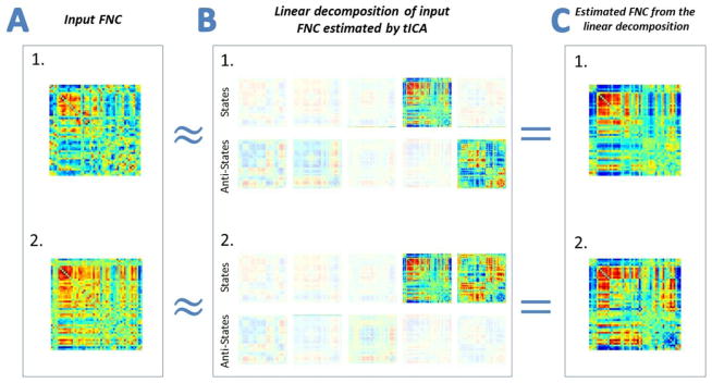
(Column A) Two instances of actual input FNC selected from the data. These instances are in fact estimated correlation matrices of windows time courses at two different time points. Linear decompositions of these FNCs, which are estimated by tICA, are shown in Column B with the amount of fading representing linear weights of each states and anti-states. Column C shows weighted sum of components from each decomposition.
3.1 Temporal ICA for explaining differences between different demographics groups
Similarly to (Rashid et al., 2014), we are also interested in explaining how various properties of dFNCs vary between different groups of subjects. We first define an occupancy measure appropriate to the expression of time-varying connectivity in terms of simultaneous contributions from multiple states or correlation patterns. We will show how such a measure can be used to study dynamical properties of these patterns, and as our main conclusion we will show that the number of different combinations of simultaneous weights on the five estimated tICA correlation patterns differ significantly according to gender.
For a typical clustering-based dFNC analysis (Allen et al., 2012) in which subjects are assigned just one best-fit state per time point from a finite collection of states, a simple property to study is the “occupancy frequency”, i.e. the number of time points each subject spends in a given state. In the case of temporally independent dFNCs, where subjects are characterized not by one state per time point, but rather by a weight for each state at each time point, the idea of occupancy is still interesting but must be adapted to the new setting. In this case one can consider the case that a certain state is ‘occupied’ at a given time by a given subject if its weight exceeds some threshold. Similarly for the anti-state it is occupied when the weight (in this case negative) exceeds in magnitude some threshold. We set the threshold for positive contribution for a given state at the 75th percentile of all positive values for time courses associated to that state (over all subjects, all time points). Positive values exceeding this threshold constitute positive occupancy of the state. Note that this allows a single subject to occupy more than one state at the same moment in time. Anti-state occupancy is treated analogously. In this case the threshold for each state is set to be the negative of the 75th percentile of the absolute values of all negative values in time courses associated to that state. We also compute an absolute occupancy measure from a 75th percentile threshold based on magnitude alone. By thresholding based on these percentile values we can easily estimate how often a given state (or its anti-state) makes a usually large contribution to subject dFNCs. We call these thresholded time course measures positive, negative and absolute occupancy frequencies which would be our new occupancy measures.
Since our data consists exclusively of healthy individuals, we are primarily interested here in studying the relationship between gender and our occupancy measure. First, for each state, we regress out the contribution of age to each of our three occupancy measures. Then we perform a 2 sample t-test between occupancy frequencies (positive, negative and absolute) of males and females (Figure 4).
Figure 4.

This figure shows the result of studying the relationship between gender and defined occupancy measure. First, for each state, we regress out the contribution of age to each of our three occupancy measures. Then we perform a 2 sample t-test between occupancy rates (positive, negative and absolute) of males and females. For each state we report which gender occupies that state more than the other and how significant the difference in occupancy measure is between the two (reported by estimated p-value after FDR adjustment). We can see, when looking at each state individually, there is no statistically significant difference between males and females with respect to their occupancy measures.
As mentioned in 1.3, one of the key benefits of our approach is that a subject can occupy more than one state at the same time, and this aspect of the occupancy behavior is worth investigating. Occupancy measure, as described above, has an integration over time and thus do not have time as one of the dimensions. However if we include co-occurrence of states into the occupancy measure we would have an implicit notion of time as well. The above analysis has not taken this fact into account. We have 5 states, each of which can, at a given moment in time, be either positively occupied (above-threshold positive time course value), negatively occupied (below threshold negative time course value) or none-occupied. This gives 35 possible co-occupancy patterns for the five states. We will call these co-occupancy patterns “combo-states” and will represent them as a base 3 number, where positive occupancy is represented with a ‘1’, negative occupancy with a ‘2’ and non-occupancy with a ‘0’ For example 0state52state40state30state21state1, or simply 02001, implies that at a given time, state 1 is positively occupied and state 4 is negatively occupied (anti-state 4 is occupied) while states 2,3 and 5 have time course values that do not exceed either the positive or negative occupancy thresholds.
Our analysis shows that out of 35 = 243 possible combo-states, only 22 of these appear more than 1% of the time. Among the 22 combo-states that occur more than 1% of the time, none involve co-occupancy of more than two states.
Figure 5 summarizes the analysis. The bar chart shows relative frequency of each combo-state occurrence. Each bar is labeled by coded and visual presentation of the associated combo-state at the bottom and at the top is labeled by the gender that on average occupies that combo-state more along with the FDR-adjusted of the p-values for comparison. On the top right corner of the figure, each slice of the pie chart shows overall occurrence frequency of the associated combo-state. We can see that although we are only showing 22 out of 243 possible combos-states they constitute about two-thirds of the overall occurrences of all combo-states. Similar to individual state analysis we do not see significant gender difference based on occupancy frequency of combo states. However, lower p-values for some combo-states such as ‘00001’, ‘02200’, ‘00102’ and ‘110010’ can be explained by having a more specific measure as a result of including co-occurrences of individual states.
Figure 5.

Bar chart shows relative occurrence frequency of each combo-state. The bottom label of each bar is the coded and visual representation of the associated combo-state and the top is labeled by the gender that one average occupies that combo-state more along with the FDR-adjusted of the p-values for that comparison (dark blue: M>F and dark red: F>M). On the top right corner of the figure, each of the pie chart shows overall occurrence frequency of the associated combo-state.
4 Discussion
Our results indicate that while neither individual state1 nor combo-state occupancy frequencies do not exhibit significant gender effects (Figure 4 and Figure 5), there are isolated individual occupancy frequencies2 and isolated co-occupancy frequencies (Figure 5) between certain pairs of states that have relatively lower p-values. This suggests that accounting for the simultaneous contributions of multiple correlation patterns to dynamical estimates of functional connectivity can increase sensitivity of the analysis to group effects. Our further investigations indicated, interestingly, that counting the number of distinct combo-states subjects pass through reveals a significant difference between men and women. After regressing out age, we found that males experience a significantly (p-value = 0.01, 2-sample, T-test) greater number of distinct combo-states than do females.
On the other hand, when we perform the analogous analysis based on individual states, i.e. counting the number of individual states (states and anti-states) that males and females go through during scan, males pick more states on average than females, but not at a significant level (p-value = 0.09, T-test).
Before concluding this discussion, it is worth mentioning that although we are looking for connectivity patterns that occur independent of each other, we are maximizing independence of these changes at the group level (minimizing mutual information between concatenated time courses in subjects and time). Our analysis of co-occurrence of states implicitly reveals that there is residual dependence at the subject level which is informative and statistically interesting. Subject-level deviation from the main assumption of group level analysis is a standard feature of many fMRI studies e.g. in spatial (Calhoun and Adali, 2012) or temporal group ICA (Seifritz et al., 2002), (Smith et al., 2012).
To better understand this, please refer to Figure 6. In this figure we simulate 5 time courses of the same size as our estimated FNC time courses taking values of 0, 1 and 2 with respectively equal occurrence probabilities of non-occupied, positively occupied and negatively occupied as estimated from original data. All of these time courses are mutually independent as their pairwise mutual information is near zero which is shown in upper triangular part of the table at the left side. However, when we look at mutual information between segments of these time courses we can see that there is considerable dependence, among these segments. Histograms of estimated mutual information between segments of each time course pairs are shown in lower triangular part of the table and we can clearly observe that these histograms are not centered at zero. In our case, these segments correspond to subject level time courses and as we have shown earlier the dependency between them is informative.
Figure 6.
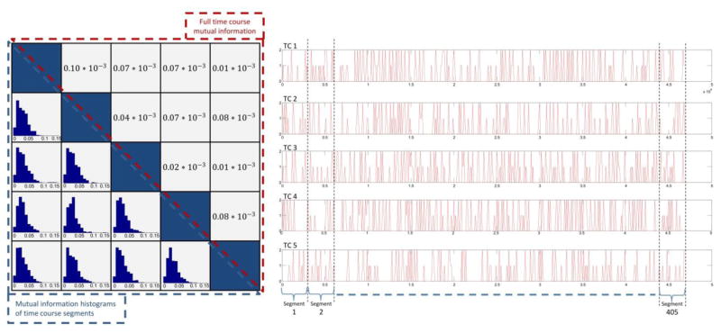
Simulation analysis of subject level deviation from group temporal independence assumption. (A) 5 time courses of the same size as our estimated FNC time courses taking values of 0, 1 and 2 with respectively equal occurrence probabilities of non-occupied, positively occupied and negatively occupied as estimated from original data. (B Upper triangular part) Calculated mutual information between all pairs of simulated time courses. (B Lower triangular part) Mutual information histograms between corresponding segments of each pairs of time courses.
However, one main difference between real and simulated data is that in real data, time courses are not truly independent at the group level either (e.g. this aspect has been exploited in previous work calculating graph metrics by utilizing the residual mutual information among component maps (Ma et al., 2012)). As is evident in Figure 7, mutual information values between pairs of full-duration time courses shown in upper triangle part of the figure, are not as close to zero as in simulated data.
Figure 7.

(Upper triangular part) Mutual information values between pairs of estimated time courses from real data. (Lower triangular part) Histograms of mutual information values of corresponding segments of each pair of estimated time course. Here each segment corresponds to a subject time course.
If temporal independence held at the group level, as it did with our simulated data, then by computing the global occurrence count of individual states, we can easily compute the occurrence count of combo-states. Under the formal independence assumption, the occurrence rate of some combo-state “yyyyy” where y ∈ {0,1,2} is equal to where r(i) is the occupancy rate of each individual state that we initially defined in section 3.1. In Figure 8 we are representing actual occurrence rate s of the 22 most commonly occurring combo-states with blue bars (same as in figure 5) along with occurrence rates of the same set of combo-states under an assumption of true temporal independence between individual states which are represented in red bars.
Figure 8.

Actual observed occurrence frequencies of most occurring combo-states (blue bars) vs. occurrence frequencies of those combo-states under true temporal independence assumption.
5 Conclusion
We have introduced mutually temporally independent connectivity patterns as a new vehicle through which to study human brain dynamics. Temporal ICA of windowed FNCs from group spatial ICA data was used to estimate such patterns, and we have explained how it is fundamentally different from currently-dominant clustering and PCA decomposition-based approaches. We introduce an occupancy measure, analogous to that used in clustering methods, adapted to fit to this new framework. By considering our method as a linear decomposition, we studied co-occurrence of the estimated connectivity patterns by introducing combo-states, and through such analysis interesting group difference based on gender was revealed. The difference became significant for the analysis of distinct number of combo-states men and women go through during rest. Our objective here was to introduce a higher-dimensional characterization of connectivity dynamics and to demonstrate its ability to find group differences. The observed gain in statistical power as our analysis moves from the individual state level, to combo-states, to collections of combo-states suggests that a higher-dimensional representation of whole-brain connectivity provides a richer information landscape in which to locate group differences.
Our proposed method shows some very interesting properties and promising results, but it is just one among many different possible ways of looking at connectivity dynamics of the brain at rest, and there is no established mechanistic physiological understanding favoring of any of these approaches. In terms of the higher-dimensional point of view we are advocating here, there are many potential directions to develop: constructing more sophisticated measures of dynamical flow through the state space could bring real gains in power and interpretability; computing connectivity patterns separately for different groups might reveal interesting differences between groups in which sets of network-pair correlations behave independently of each other, and different ways of decomposing the data (for instance, finding connectivity patterns that are mutually spatially independent rather than mutually temporally independent) might be useful for certain types of questions.
Highlights.
Introduction of mutually temporally independent connectivity patterns as a new framework to study brain dynamics in rest
Introduction of a new occupancy and co-occurrence measure that fits to this framework
Explaining gender differences based on occupancy and co-occurrence measures of such connectivity patterns
Acknowledgments
We thank the multiple MRN investigators who collected the data (more details are provided in (Allen et al., 2011)). This study was funded by a Center of Biomedical Research Excellence (COBRE) grant 5P20RR021938/P20GM103472 from the NIH to Dr. Vince Calhoun.
Abbreviations
- ICA
Independent Component Analysis
- FC
Functional Connectivity
- FNC
Functional Network Connectivity
Footnotes
Individual state occupancy is when a certain state is occupied (based on our former definition of occupancy) regardless of other states. For example individual occupancy of state 1 is the integral of occupancy over all combo-states of the form [y y y y 1] where y ∈ |0 1 2|. Individual states correspond to states shown in Figure 4.
Isolated individual state occupancy is when a certain state is occupied while other states are not. For example isolated individual occupancy of state 1 is occupancy of combo-state of the form [0 0 0 0 1]. This definition can be extended to any instances of states co-occupancies. For example isolated co-occupancy of states 1 and 2 is occupancy of combo-state [0 0 0 1 1].
The authors declare no conflict of interest.
Publisher's Disclaimer: This is a PDF file of an unedited manuscript that has been accepted for publication. As a service to our customers we are providing this early version of the manuscript. The manuscript will undergo copyediting, typesetting, and review of the resulting proof before it is published in its final citable form. Please note that during the production process errors may be discovered which could affect the content, and all legal disclaimers that apply to the journal pertain.
References
- Allen EA, Damaraju E, Plis SM, Erhardt EB, Eichele T, Calhoun VD. Tracking Whole-Brain Connectivity Dynamics in the Resting State. Cereb Cortex. 2012 doi: 10.1093/cercor/bhs352. [DOI] [PMC free article] [PubMed] [Google Scholar]
- Allen EA, Erhardt EB, Damaraju E, Gruner W, Segall JM, Silva RF, Havlicek M, Rachakonda S, Fries J, Kalyanam R, Michael AM, Caprihan A, Turner JA, Eichele T, Adelsheim S, Bryan AD, Bustillo J, Clark VP, Feldstein Ewing SW, Filbey F, Ford CC, Hutchison K, Jung RE, Kiehl KA, Kodituwakku P, Komesu YM, Mayer AR, Pearlson GD, Phillips JP, Sadek JR, Stevens M, Teuscher U, Thoma RJ, Calhoun VD. A baseline for the multivariate comparison of resting-state networks. Front Syst Neurosci. 2011;5:2. doi: 10.3389/fnsys.2011.00002. [DOI] [PMC free article] [PubMed] [Google Scholar]
- Beckmann CF, DeLuca M, Devlin JT, Smith SM. Investigations into resting-state connectivity using independent component analysis. Philosophical Transactions of the Royal Society B-Biological Sciences. 2005;360:1001–1013. doi: 10.1098/rstb.2005.1634. [DOI] [PMC free article] [PubMed] [Google Scholar]
- Bressler SL, Menon V. Large-scale brain networks in cognition: emerging methods and principles. Trends Cogn Sci. 2010;14:277–290. doi: 10.1016/j.tics.2010.04.004. [DOI] [PubMed] [Google Scholar]
- Bullmore E, Sporns O. Complex brain networks: graph theoretical analysis of structural and functional systems. Nat Rev Neurosci. 2009;10:186–198. doi: 10.1038/nrn2575. [DOI] [PubMed] [Google Scholar]
- Calhoun VD, Adali T. Multisubject independent component analysis of fMRI: a decade of intrinsic networks, default mode, and neurodiagnostic discovery. IEEE Rev Biomed Eng. 2012;5:60–73. doi: 10.1109/RBME.2012.2211076. [DOI] [PMC free article] [PubMed] [Google Scholar]
- Calhoun VD, Adali T, Pearlson GD, Pekar JJ. A method for making group inferences from functional MRI data using independent component analysis. Hum Brain Mapp. 2001a;14:140–151. doi: 10.1002/hbm.1048. [DOI] [PMC free article] [PubMed] [Google Scholar]
- Calhoun VD, Adali T, Pearlson GD, Pekar JJ. Spatial and temporal independent component analysis of functional MRI data containing a pair of task-related waveforms. Hum Brain Mapp. 2001b;13:43–53. doi: 10.1002/hbm.1024. [DOI] [PMC free article] [PubMed] [Google Scholar]
- Calhoun Vince D, Miller R, Pearlson G, Adal T. The Chronnectome: Time-Varying Connectivity Networks as the Next Frontier in fMRI Data Discovery. Neuron. 2014;84:262–274. doi: 10.1016/j.neuron.2014.10.015. [DOI] [PMC free article] [PubMed] [Google Scholar]
- Chang C, Glover GH. Time-frequency dynamics of resting-state brain connectivity measured with fMRI. Neuroimage. 2010;50:81–98. doi: 10.1016/j.neuroimage.2009.12.011. [DOI] [PMC free article] [PubMed] [Google Scholar]
- Damaraju E, Allen EA, Belger A, Ford J, McEwen SC, Mathalon D, Mueller B, Pearlson GD, Potkin SG, Preda A, Turner J, Vaidya JG, Van Erp T, Calhoun VD. Dynamic functional connectivity analysis reveals transient states of dysconnectivity in schizophrenia. Neuroimage: Clinical. 2014 doi: 10.1016/j.nicl.2014.07.003. [DOI] [PMC free article] [PubMed] [Google Scholar]
- Damoiseaux JS, Rombouts SARB, Barkhof F, Scheltens P, Stam CJ, Smith SM, Beckmann CF. Consistent resting-state networks across healthy subjects. Proceedings of the National Academy of Sciences of the United States of America. 2006;103:13848–13853. doi: 10.1073/pnas.0601417103. [DOI] [PMC free article] [PubMed] [Google Scholar]
- Erhardt EB, Allen EA, Damaraju E, Calhoun VD. On network derivation, classification, and visualization: a response to Habeck and Moeller. Brain Connect. 2011a;1:1–19. [PMC free article] [PubMed] [Google Scholar]
- Erhardt EB, Rachakonda S, Bedrick EJ, Allen EA, Adali T, Calhoun VD. Comparison of Multi-Subject ICA Methods for Analysis of fMRI Data. Hum Brain Mapp. 2011b;32:2075–2095. doi: 10.1002/hbm.21170. [DOI] [PMC free article] [PubMed] [Google Scholar]
- Fox MD, Greicius M. Clinical applications of resting state functional connectivity. Front Syst Neurosci. 2010;4:19. doi: 10.3389/fnsys.2010.00019. [DOI] [PMC free article] [PubMed] [Google Scholar]
- Friedman J, Hastie T, Tibshirani R. Sparse inverse covariance estimation with the graphical lasso. Biostatistics. 2008;9:432–441. doi: 10.1093/biostatistics/kxm045. [DOI] [PMC free article] [PubMed] [Google Scholar]
- Himberg J, Hyvarinen A. ICASSO: Software for investigating the reliability of ICA estimates by clustering and visualization. 2003 Ieee Xiii Workshop on Neural Networks for Signal Processing - Nnsp’03; 2003. pp. 259–268. [Google Scholar]
- Hutchison RM, Womelsdorf T, Allen EA, Bandettini PA, Calhoun VD, Corbetta M, Della Penna S, Duyn JH, Glover GH, Gonzalez-Castillo J, Handwerker DA, Keilholz S, Kiviniemi V, Leopold DA, de Pasquale F, Sporns O, Walter M, Chang C. Dynamic functional connectivity: promise, issues, and interpretations. Neuroimage. 2013;80:360–378. doi: 10.1016/j.neuroimage.2013.05.079. [DOI] [PMC free article] [PubMed] [Google Scholar]
- Jafri MJ, Pearlson GD, Stevens M, Calhoun VD. A method for functional network connectivity among spatially independent resting-state components in schizophrenia. Neuroimage. 2008;39:1666–1681. doi: 10.1016/j.neuroimage.2007.11.001. [DOI] [PMC free article] [PubMed] [Google Scholar]
- Kilpatrick LA, Zald DH, Pardo JV, Cahill LF. Sex-related differences in amygdala functional connectivity during resting conditions. Neuroimage. 2006;30:452–461. doi: 10.1016/j.neuroimage.2005.09.065. [DOI] [PubMed] [Google Scholar]
- Kiviniemi V, Vire T, Remes J, Elseoud AA, Starck T, Tervonen O, Nikkinen J. A sliding time-window ICA reveals spatial variability of the default mode network in time. Brain Connect. 2011;1:339–347. doi: 10.1089/brain.2011.0036. [DOI] [PubMed] [Google Scholar]
- Leonardi N, Richiardi J, Gschwind M, Simioni S, Annoni JM, Schluep M, Vuilleumier P, Van De Ville D. Principal components of functional connectivity: a new approach to study dynamic brain connectivity during rest. Neuroimage. 2013;83:937–950. doi: 10.1016/j.neuroimage.2013.07.019. [DOI] [PubMed] [Google Scholar]
- Lynall ME, Bassett DS, Kerwin R, McKenna PJ, Kitzbichler M, Muller U, Bullmore E. Functional Connectivity and Brain Networks in Schizophrenia. Journal of Neuroscience. 2010;30:9477–9487. doi: 10.1523/JNEUROSCI.0333-10.2010. [DOI] [PMC free article] [PubMed] [Google Scholar]
- Ma S, Calhoun VD, Eichele T, Du W, Adali T. Modulations of functional connectivity in the healthy and schizophrenia groups during task and rest. Neuroimage. 2012;62:1694–1704. doi: 10.1016/j.neuroimage.2012.05.048. [DOI] [PMC free article] [PubMed] [Google Scholar]
- Majeed W, Magnuson M, Hasenkamp W, Schwarb H, Schumacher EH, Barsalou L, Keilholz SD. Spatiotemporal dynamics of low frequency BOLD fluctuations in rats and humans. Neuroimage. 2011;54:1140–1150. doi: 10.1016/j.neuroimage.2010.08.030. [DOI] [PMC free article] [PubMed] [Google Scholar]
- Rashid B, Damaraju E, Pearlson GD, Calhoun VD. Dynamic Connectivity States Estimated from Resting fMRI Identify Differences among Schizophrenia, Bipolar Disorder, and Healthy Control Subjects. Frontiers in Human Neuroscience. 2014:8. doi: 10.3389/fnhum.2014.00897. [DOI] [PMC free article] [PubMed] [Google Scholar]
- Sakoğlu ğ, Pearlson Godfrey D, Kiehl Kent A, Michelle Wang Y, Michael Andrew M, Vince D Calhoun. A method for evaluating dynamic functional network connectivity and task-modulation: application to schizophrenia. Magnetic Resonance Materials in Physics, Biology and Medicine. 2010;23:351–366. doi: 10.1007/s10334-010-0197-8. [DOI] [PMC free article] [PubMed] [Google Scholar]
- Seifritz E, Esposito F, Hennel F, Mustovic H, Neuhoff JG, Bilecen D, Tedeschi G, Scheffler K, Di Salle F. Spatiotemporal pattern of neural processing in the human auditory cortex. Science. 2002;297:1706–1708. doi: 10.1126/science.1074355. [DOI] [PubMed] [Google Scholar]
- Smith SM, Miller KL, Moeller S, Xu J, Auerbach EJ, Woolrich MW, Beckmann CF, Jenkinson M, Andersson J, Glasser MF, Van Essen DC, Feinberg DA, Yacoub ES, Ugurbil K. Temporally-independent functional modes of spontaneous brain activity. Proc Natl Acad Sci U S A. 2012;109:3131–3136. doi: 10.1073/pnas.1121329109. [DOI] [PMC free article] [PubMed] [Google Scholar]