

Abstract
Objective
Auditory subcortical steady state responses (SSSRs), also known as frequency following responses (FFRs), provide a non-invasive measure of phase-locked neural responses to acoustic and cochlear-induced periodicities. SSSRs have been used both clinically and in basic neurophysiological investigation of auditory function. SSSR data acquisition typically involves thousands of presentations of each stimulus type, sometimes in two polarities, with acquisition times often exceeding an hour per subject. Here, we present a novel approach to reduce the data acquisition times significantly.
Methods
Because the sources of the SSSR are deep compared to the primary noise sources, namely background spontaneous cortical activity, the SSSR varies more smoothly over the scalp than the noise. We exploit this property and extract SSSRs efficiently, using multichannel recordings and an eigendecomposition of the complex cross-channel spectral density matrix.
Results
Our proposed method yields SNR improvement exceeding a factor of 3 compared to traditional single-channel methods.
Conclusions
It is possible to reduce data acquisition times for SSSRs significantly with our approach.
Significance
The proposed method allows SSSRs to be recorded for several stimulus conditions within a single session and also makes it possible to acquire both SSSRs and cortical EEG responses without increasing the session length.
Keywords: Multichannel, Frequency following response, Auditory brainstem response, Complex principal component analysis, Rapid acquisition
1. Introduction
Subcortical steady state responses (SSSRs), frequently referred to as frequency following responses (FFRs), are the scalp-recorded responses originating from sub-cortical portions of the auditory nervous system. These responses phase lock to periodicities in the acoustic waveform and to periodicities induced by cochlear processing (Glaser et al., 1976). The responses specifically phase locked to the envelopes of amplitude modulated sounds are sometimes called amplitude modulation following responses (AMFRs) or envelope following responses (EFRs) (Dolphin and Mountain, 1992; Kuwada et al., 2002). Responses to amplitude-modulated sounds originating from both the sub-cortical and cortical portions of the auditory pathway are also collectively referred to as auditory steady-state responses (ASSR) (Rees et al., 1986). In contrast to auditory brainstem responses (ABRs; the stereotypical responses to sound onsets and offsets; Jewett et al., 1970), SSSRs are the sustained responses to ongoing sounds and include responses phase-locked to both the fine structure and the cochlear induced envelopes of broadband sounds. Since the term FFR, originally used to denote phase locked responses to pure tones, is suggestive of responses phase-locked to the fine-structure of narrowband or locally narrowband sounds, here we will use the term SSSR to describe the sustained responses originating from subcortical portions of the auditory pathway. This name distinguishes them from transient onset-offset related responses and responses generated at the cortical level. SSSRs have been used extensively in basic neurophysiologic investigation of auditory function and sound encoding (e.g. Aiken and Picton, 2008; Kuwada et al., 1986; Gockel et al., 2011 also see Chandrasekaran and Kraus, 2010; Krishnan et al., 2006; Picton et al., 2003, for reviews). Given the frequency specificity possible with SSSRs, they have also been recommended for objective clinical audiometry (Lins et al., 1996).
SSSRs are traditionally recorded with a single electrode pair placed in either a vertical or a horizontal montage (which differ in which underlying generators are emphasized; see Krishnan et al., 2006, 2010). To achieve an adequate signal-to-noise ratio (SNR) when measuring the SSSR, the stimulus is typically repeated thousands of times. Often, stimuli are presented in opposite polarities to separate the response components phase locked to the envelope from those phase locked to the fine structure of the acoustic waveform (Aiken and Picton, 2008; Ruggles et al., 2012). Since many studies require SSSR data acquisition for multiple conditions or with multiple stimuli, this often results in recording sessions exceeding an hour per subject.
Multichannel electroencephalography (EEG), which is widely used for the investigation of cortical processing, uses the same basic sensors as SSSR measurements, but requires many fewer trials because the cortical response generators are closer to the scalp and produce stronger electric fields. EEG systems with high-density arrays include as many as 64, 128, or sometimes even 256 scalp electrodes. Although the frequency response characteristics of some cortical EEG systems are not always optimized for picking up subcortical signals (which typically are at 80 Hz and above), these multi-electrode setups can nonetheless be used to record SSSR data from multiple scalp locations.
Given this, it is possible to simultaneously record subcortical and cortical processing of sounds with the high-frequency portions analyzed to yield SSSRs and the low-frequency portions representing cortical activity (Krishnan et al., 2012). The primary source of noise for the high-frequency SSSR portion of the recordings is background cortical activity (i.e., neural noise). Since the SSSR sources are deep compared to the dominant sources of noise (in the cortex), the SSSR varies more smoothly over the scalp than the noise (for a discussion of the physics of the measurement process and how scalp fields relate to neural activity, see Hämäläinen et al., 1993). Scalp fields arising from cortical sources can cancel each other out if they are out of phase (Irimia et al., 2012). This can be exploited to help separate cortical and subcortical responses from the same EEG recordings by combining information obtained from a dense sensor array. Here, we propose and evaluate one method for combining measurements from multiple scalp channels to improve the SNR of SSSRs measured using cortical EEG arrays.
Although SSSRs can provide insight into auditory function and subcortical encoding, interpreting them can be a challenge. Multichannel recordings of brainstem responses have been used primarily in the analysis of the sources of the onset ABR, in which the activity from different generators can be temporally separated, into stereotypical responses known as waves I, III, and V (Grandori, 1986; Parkkonen et al., 2009; Scherg and Von Cramon, 1986). In contrast, since the SSSRs represent sustained activity, temporal separation of the activity from different generators is not possible. Moreover, in any narrow frequency band, particularly at high frequencies, multiple SSSR sources likely contribute to the aggregate measured response, each of which is a phase-locked response at a different phase. This notion is consistent with the observation that there are spectral notches and occasional phase discontinuities in the SSSR as a function of modulation frequency for amplitude modulated stimuli (Dolphin and Mountain, 1992; Kuwada et al., 2002; Purcell et al., 2004). This is also consistent with the observation that responses are attenuated but not eliminated in studies inducing isolated lesions of single auditory nuclei (Smith et al., 1975; Kiren et al., 1994). This multisource population activity produces scalp potentials that are different mixtures of the source activity at different scalp locations, depending on the geometry of the generators, the recording electrodes, and the volume conductor in between (Hubbard et al., 1971; Okada et al., 1997; Irimia et al., 2013). Consistent with this notion, the steady-state phase of the summed, observed response at a given frequency varies across different channels, as illustrated in Fig. 1.
Fig. 1.
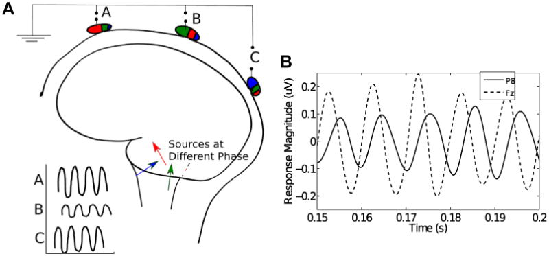
(A) A schematic illustration of the possible origin of phase differences of the SSSR recorded from different scalp electrodes. Each neural generator, shown as three different colored arrows, is phased-locked to the stimulus, but at a different unique phase. Moreover, the generators contribute different amounts to different scalp locations, as illustrated by the proportion of the ellipses shaded with the corresponding colors. This results in phase misalignment between the effective total response at different recording sites. (B) Real SSSR obtained from a typical subject from two distinct scalp locations (relative to the average potential between the two earlobes) showing phase differences in the response. The data is filtered between 90 and 110 Hz to emphasize the response at the fundamental stimulus frequency of 100 Hz. (For interpretation of the references to colour in this figure legend, the reader is referred to the web version of this article.)
Unfortunately, time-domain methods to combine multichannel recordings, such as simple across electrode averaging or principal component analysis (PCA), assume that the signal is at the same phase across sensors. For instance, time-domain PCA involves recombination of multiple measurements with real-valued weights based on the covariance matrix. As a result, these methods lead to signal attenuation when the signal components in each sensor are not at the same phase. In other fields of analysis, complex principal component analysis (cPCA) in the frequency domain has been used to effectively combine multiple measurements when the signal components are correlated, but have phase differences (Brillinger, 1981; Horel, 1984). In contrast to traditional time-domain PCA, frequency domain cPCA recombines measurement channels using the complex-valued weights obtained by decomposing the complex cross-channel spectral density matrix. The weights thus include channel-specific magnitudes and phases in each frequency bin; the phases of each complex weight specifically adjust for phase differences between responses measured at different sites to optimally combine responses across multiple sensors. Here we apply cPCA to multichannel EEG recordings, thereby accounting for phase discrepancies across the scalp and extract SSSRs efficiently. We show that compared to single-channel recording, this approach reduces the data acquisition required to achieve the same SNR, both when applied to simulations and when analyzing real multichannel SSSR recordings.
2. Methods
First, we describe the steps involved in the cPCA method. Then, we describe our procedure to validate the method using simulated data. Finally, using EEG-data acquired from normal-hearing human listeners, we demonstrate how to apply the approach to extract SSSRs from multi-electrode recordings.
2.1. Complex principal component analysis (cPCA)
Frequency-domain PCA can be used to effectively reduce the dimensionality of vector-valued time-series in the presence of between-component dependencies at delayed time intervals (Brillinger, 1981). As illustrated in Fig. 1, for any frequency component, responses at different scalp locations occur with different effective phases. This is unlikely to be due to conduction delays between the recording site and the sources since the brain tissue and head together can be treated as a pure conductor (no capacitive effects) for frequencies below about 20 kHz. That is, the forward model that relates the measured potentials to the source currents can be treated as quasi-static (Hämäläinen et al., 1993). Because each subcortical source contributes a different amount to each scalp sensor, depending on their geometry relative to the recording electrodes, the shapes and conductivity profiles of the different tissues in between, the choice of reference etc. (Hubbard et al., 1971; Okada et al., 1997; Irimia et al., 2013), the resultant signal in each sensor will have a different phase. For multivariate time-series, the cross-spectral density matrix captures up to second-order dependencies between the individual components of the time-series, and therefore has information we can exploit to account for these phase differences in the signal across the sensors. First, we apply a discrete prolatespheroidal taper sequence, wk(t), to the recorded/simulated signals (Slepian, 1978). We then estimate the complex-cross channel spectral density matrix, M(f), at each frequency bin, from which we estimate the principal eigenvalue, λk(f), and the corresponding eigenweights, vk(f), using a diagonalization procedure. For a given frequency resolution, the use of the Slepian taper minimizes the bias introduced due leakage of frequency content from other frequencies outside the resolution bandwidth into the estimate of the passband content (Thomson, 1982). Consequently, the Slepian taper minimizes the bias in the estimates of the eigenvalues, λ(f), which result from the spectra being colored (Brillinger, 1981). Thus, for recording epochs of duration T, we have:
| (1) |
| (2) |
where Xi(f) denotes the tapered Fourier transform of the data χi(t) in the ith recording channel, Mij(f) denotes the cross-spectrum between channels i and j, corresponding to the ijth element of the full cross-channel spectral density matrix M(f), superscript * denotes complex-conjugate, and 〈.〉 denotes averaging over trials. The tapers wk, k = 1, 2,…, Ntap form an approximate basis for signals that are limited to a duration-bandwidth product of 2TW, and satisfy an eigenvalue equation:
| (3) |
where the eigenvalues ck ≈ 1 for k ≤ Ntap = 2TW − 1 are the concentrations of the tapers within the band −W ≤ f ≤ W (Slepian, 1978). The estimates of λk(f) obtained using the Ntap tapers (indexed by k) are then averaged together to reduce the variance of the estimate without additional bias from spectral leakage from frequencies outside of the bandwidth W:
| (4) |
By construction, M(f) is Hermitian and positive semi-definite. Thus, M(f) has real, non-negative eigenvalues, and can be diagonalized using a Cholesky factorization procedure:
| (5) |
where Q(f) is the unitary matrix of complex eigenvectors of M(f), Λ(f) is the diagonal matrix of real eigenvalues and superscript H denotes conjugate-transpose. Note that a separate cross-channel spectral density matrix is estimated at each frequency bin and the eigendecomposition is also performed at each frequency bin separately. This is not redundant because, by the central limit theorem, for a stationary signal, the estimated frequency coefficients are uncorrelated and asymptotically Gaussian distributed. The principal eigenvalue λ(f) = Λ11(f) estimates the power spectrum of the first principal component signal (Brillinger, 1981) and the phase of the corresponding eigenvector v(f) = Q.1(f) estimates the phase delays that need to be applied to individual channels in order to maximally align them. Here Q.1 denotes the first column vector of Q, composed of the first element of all the rows of the matrix.
SSSRs are often appropriately analyzed in the frequency domain as they represent steady-state mixtures of subcortical source activity (Aiken and Picton, 2006; Aiken and Picton, 2008; Galbraith et al., 2000; Gockel et al., 2011; Krishnan, 1999; Krishnan, 2002; Wile and Balaban, 2007). The eigendecomposition of the cross-spectral matrix is thus convenient for SSSR analysis in the sense that the principal eigenvalue directly provides a metric of the SSSR power at a given frequency without further processing being necessary. Moreover, the phase-locking value (PLV) (Lachaux et al., 1999) is a normalized, easily interpreted measure of across-trial phase locking of the SSSR at different frequencies and also has convenient statistical properties (Dobie and Wilson, 1993; Zhu et al., 2013). The use of the normalized cross-spectral density matrix Cplv(f) (see below) instead of M(f) allows for the direct estimation of PLV through the eigendecomposition. An analogous modification can be used to obtain estimates of inter-trial coherence (ITC) (see Delorme and Makeig, 2004 see Delorme and Makeig, 1994) by using Citc(f), as defined below:
| (6) |
| (7) |
where Cij(f) denotes the ijth element of the corresponding normalized cross-spectral density matrix C(f) and 〈.〉 denotes averaging over trials. The set p(f) of the largest eigenvalues of C(f) at each frequency bin then provides the PLV or the ITC of the corresponding first principal component directly. The variance of the PLV and ITC estimates depend only on the number of trials included in the estimation (Bokil et al., 2007; Zhu et al., 2013). In the absence of a phase-locked signal component, both the mean (bias) and the variance of the estimated PLV (i.e., the noise floor) are directly related to the number of trials. Taking advantage of this, in order to compare the SNR obtained using the cPCA method to the SNR from a single channel and from time-domain PCA, we normalize the PLV measure so that the noise floor is approximately normally distributed with a zero-mean and unit variance:
| (8) |
where μnoise and σnoise denote the sample mean and standard deviation of the noise floor estimated from the PLV or the ITC spectrum p(f) using a bootstrap procedure (Zhu et al., 2013). Alternately, similar estimates of noise can be obtained from p(f) by excluding the frequency bins that have stimulus-driven response components. PLVz(f) gives the PLV as a function of frequency measured in z-scores relative to the noise floor and hence quantifies the SNR obtained using different methods, allowing them to be compared directly.
2.2. Simulations
Simulated SSSR recordings were produced by generating 32 channels of data with each containing a 200 ms burst of a 100 Hz sinusoid at a different randomly chosen phase (distributed uniformly around the circle). Background EEG-like noise was added to generate 200 simulated trials of raw EEG data. The noise had the same spectrum and spatial (between-channel) covariance as resting state EEG (note that the background cortical EEG activity is itself one of the primary sources of noise for SSSR measurements). The phase of the 100 Hz sinusoid (the SSSR signal of interest), though not aligned across channels, was kept constant across trials within each channel. The root-mean-squared (RMS) SNR for a single trial in each channel was set at −40 dB. This is comparable to typical SNRs for SSSRs obtained with our EEG setup, where the SSSR amplitude is typically on the order of hundreds of nanovolts, while the background, narrowband EEG amplitude is on the order of tens of microvolts. The SSSR was then extracted from the simulated data using traditional time-domain PCA as well as cPCA.
2.3. EEG data
2.3.1. Participants
Nine participants aged 20–40 were recruited from the Boston University community in accordance with procedures approved by the Boston University Charles River Campus Institutional Review Board and were paid for their participation. For all subject, pure-tone audiometric thresholds were measured from 250 to 8000 Hz at octave intervals. All participants had hearing thresholds within 15 dB of normal hearing level in each ear at all tested frequencies, and none had any history of central or peripheral hearing deficits.
2.3.2. Stimuli, data acquisition and processing
Stimuli were generated offline in MATLAB (Natick, MA) and stored for playback using a sampling rate of 48,828 Hz. Each trial consisted of a train of 72 μs-long clicks presented at a repetition rate of 100 Hz for a burst period of 200 ms. The inter-trial interval was random and uniformly distributed between 410 and 510 ms. This 100 ms jitter ensured that EEG noise that is not in response to the stimulus occurs at a random phase between −π and π for frequencies above 10 Hz. For eight of the nine participants, for a randomly chosen set of 500 out of the 1000 trials presented, the polarity of the click-trains was reversed. This allows responses phase-locked to the cochlear-induced envelopes to be separated from the responses phase-locked to the temporal fine structure of the acoustic input (Aiken and Picton, 2008; Ruggles et al., 2011). For one participant, the total number of trials was increased to 1500 (half presented in each polarity) to allow for a more detailed analysis of how the noise level varied with the number of trials for different analysis approaches (see Section 2.3.3). Scalp responses to the click-train stimuli were recorded in 32 channels at a sampling rate of 16,384 Hz in a sound-shielded room using a BioSemi ActiveTwo EEG system. The measurements were then re-referenced offline to the average potentials recorded at the two earlobes using additional surface electrodes. An additional reference electrode was placed on the seventh cervical vertebra (C7) to allow for offline construction of a vertical montage channel for comparison (Gockel et al., 2011; Krishnan et al., 2006; Marsh et al., 1975). The continuous recording from each electrode was high-pass filtered in MATLAB at 70 Hz using an FIR filter with zero group-delay to minimize signal contributions from cortical sources before epoching (Kuwada et al., 2002; Dolphin and Mountain, 1992; Herdman et al., 2002). Response epochs from −50 to 250 ms relative to the stimulus onset time of each trial were segmented out from each channel with the epochs going from −50 to 250 ms relative to the stimulus onset time of each trial, resulting in 300 ms long epochs. Epochs with signals whose dynamic range exceeded 50μV in any channel were excluded from further analysis to remove movement and muscle activity artifacts.
2.3.3. Analysis
The epoched 32 channel data were processed using the cPCA method described above to provide estimates of PLV and PLVz. In order to taper the 300 ms long epochs for frequency analysis, the time-bandwidth product was set to obtain a resolution 2W = 6:66 Hz in the frequency domain. This allowed the use of one Slepian taper that had a spectral concentration c ≈ 1. The vertical-montage single channel (Fz - C7) was used for comparison. In addition to comparing the cPCA result to the single channel, we also combined the 32 channels using traditional time-domain PCA and estimated the PLV from the combined result. Two separate analyses were performed to (1) compare the SNR across single-channel, time-domain PCA and the cPCA methods and (2) to estimate the number of cPCA trials needed using the cPCA method to roughly obtain similar noise floor levels as the single-channel approach for individual subject results.
To compare the SNR across methods for a given number of trials, a bootstrapping procedure (Ruggles et al., 2011; Zhu et al., 2013) was used to generate estimated PLV distributions for each analysis approach that are approximately Gaussian distributed. This allowed simple, direct comparisons across the analysis methods. For each method (vertical montage, time-domain PCA and cPCA), 200 trials of each polarity were drawn at random 800 times with replacement and the PLV values estimated for each draw. The PLV estimates from different draws were then averaged in order to make the result more normally distributed before transforming them to z-scores to yield PLVz(f). The value of the z-score at the fundamental frequency (F0 = 100 Hz) was used as a measure of SNR, given that the noise distributions were equalized across the different methods. We then systematically evaluated the effect of increasing the number of recording channels on the SNR of the extracted SSSRs.
In order to get an idea of the number of trials needed to obtain similar noise-floor levels as the more traditional, single-channel approaches at the level of an individual subject, we estimated the noise floor for a fixed pool of trials from the one subject for whom we measured responses to 1500 trials. For this analysis, we parametrically varied the number of trials we analyzed to determine how the noise floor varied with the trial pool size. The overall procedure is described step by step as follows:
Fix the analysis pool to the first Npool trials acquired from the subject.
From the fixed pool of Npool trials, draw Npool trials with replacement.
For each draw, estimate the PLV spectrum using the cPCA method or for the vertical montage channel.
Repeat the drawing (with replacement) and PLV estimation procedure for a total of M draws with the same fixed pool of Npool trials.
-
Estimate the variance of the noise floor σ2 (Npool), for the fixed pool of trials using the plugin formula (Bickel and Freedman, 1981)
(9) where s2 is the sample sum of squared central deviations over the M draws.
Repeat the procedure for different pool sizes by progressively increasing Npool to obtain the noise-floor estimate curves for the cPCA and the single-channel methods.
We performed this analysis while varying Npool from 100 to 1500 in steps on 50, with the variance estimate calculated using M = 50 draws for each trial pool. By using an individual subject's data and by fixing the pool of trials at each stage, this procedure allows us to estimate how many trials are needed using a given analysis method to achieve a given amount of noise suppression. This analysis also allows us to compare the noise floor obtained using the traditional single-channel montage with that obtained using our multichannel approach, for a fixed number of trials.
3. Results
3.1. Simulations
Fig. 2A show sample SSSRs obtained by averaging 200 trials on a single channel (top panel), using time-domain PCA (middle panel), and using the cPCA methods (bottom panel). Though the SSSR extracted by time-domain PCA shows some improvement in SNR relative to using a single electrode, the gain in SNR using the cPCA method is greater. This is further elucidated in Fig. 3A, which shows the relationship between the phase delays estimated using the cPCA method and the original simulated phase delays for a typical simulation. The estimated signal phase at a given channel corresponds very closely to the true simulated phase of the signal in that channel. This shows that the complex eigenweights v(f) obtained from the cross-channel spectral density matrix M(f) capture the relative phase shifts between the individual channels. Fig. 3B shows the relationship between the errors in the estimation of phase shift and the magnitude of the eigenweights across the different channels. The magnitude of the phase estimation error is inversely related to the channel weight magnitudes. This result shows that the channels with poor SNR have the largest phase estimation errors. Thus, using this method, the relative contribution of a given channel to the final extracted SSSR and estimate of PLV depends on the reliability of the channel; the channels that have poorly estimated phases contribute relatively little to the final signal estimate. Finally, an assessment of the number of significant principal components shows that, in contrast to time-domain PCA, where multiple components are needed to capture all signal energy (top panel of Fig. 2B), with the cPCA method, the majority of the signal energy is captured by the single extracted principal component (bottom panel of Fig. 2B). This makes sense, given that the only parameters that distinguish between channels, namely the channel SNR and relative phase, are both accounted for by the complex weight vector obtained in the cPCA method. The magnitudes of the eigenweights account for the relative SNRs and between-channel correlations; the phase of the eigenweights accounts for the discrepancies in the phase alignment.
Fig. 2.

Simulation results: (A) The trial-averaged response at a single simulated channel (top panel), the extracted SSSR using time-domain PCA (middle panel), and the extracted SSSR using cPCA (bottom panel) are shown. Though the time-domain PCA has a greater SNR compared to any single channel, the cPCA method produces SSSRs of significantly higher SNR than does time-domain PCA. (B) The normalized eigenweights for the different principal components using traditional time-domain PCA (top panel) and cPCA (bottom panel) for the simulated EEG data. The cPCA method captures most of the signal energy in one component, showing that one weight vector accounts for both the magnitude and phase variations across channels.
Fig. 3.

Simulation results: (A) Relationship between the true simulated phase and the phase shifts estimated using the cPCA method for a typical simulation. The cPCA method produces accurate estimates of the phase delay necessary to align the channels. (B) Phase estimation errors are inversely related to the channel weights (shown for a typical simulation). Specifically, the channels with larger phase estimation error have a lower relative weight, and hence contribute weakly to the final extracted SSSR, while channels with accurately estimated phases are weighted more strongly.
3.2. Human EEG data
We applied the cPCA method to SSSR recordings obtained in response to click trains with a fundamental frequency of 100 Hz and harmonics up to 10 kHz. Estimates of the cross-channel spectral density matrices were obtained using 300 ms epochs and a time-bandwidth product of 2. This yielded an estimate of the complex cross-spectral density matrix M(f), with a frequency resolution of 6:66 Hz. For a different, larger choice of frequency resolution, multiple, orthogonal tapers can be obtained that have the same time-bandwidth product, providing a multitapered estimate. Here, we used only a single taper, yielding the maximum possible frequency resolution.
The top, middle, and bottom panels of Fig. 4A show the SSSR phase locking values obtained using the vertical montage channel, traditional time-domain PCA, and cPCA, respectively, for a representative subject. All three methods produced comparable phase-locking estimates. However, analogous to the simulation results, the variance of the noise floor (seen at the non-harmonic frequency bins where there is no signal) for the individual channnels and the traditional PCA method were significantly higher than for the cPCA method. This is quantified for all nine subjects in Fig. 4B, which shows the variance of the noise floor for the single-channel montage and for the multichannel estimate using the cPCA method. It is clear from visual inspection that for each subject, the cPCA method using 32 channels reduced the noise-floor variance, rendering the stimulus-related response peaks at the fundamental and harmonic frequencies more easily distinguishable from the noise floor.
Fig. 4.
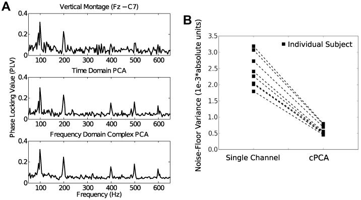
(A) Raw phase-locking value (PLV) scores obtained from a representative subject using a single channel (top), time-domain PCA (middle), and cPCA (bottom) for a 100 Hz click-train burst stimulus. The PLV obtained using the three methods are comparable at signal frequencies (multiples of 100 Hz), but differ in the variability of the noise floor. The cPCA method hence produces PLV values that are statistically more robust than the other methods. (B) The noise floor variance estimated using the bootstrap procedure is shown for each of the nine subjects for the single-channel montage and for the multichannel estimate using the cPCA method. It is clear from visual inspection, and confirmed using the permutation procedure, that the noise-variance was smaller using cPCA that for the other methods for every subject, rendering the responses more easily distinguishable from noise.
This was tested statistically using a permutation procedure; the variances of the PLV estimates (one estimate per subject per method, i.e. three numbers per subject) obtained from the bootstrap PLV procedure for the different analysis methods (single-channel, time-domain PCA and cPCA; labelled method) were pooled together. For every subject, the method labels associated with the three variance estimates were randomly permuted. For each permutation, the within-subject difference in variance between pairs of methods was calculated. These within subject variance differences between method pairs were pooled across subjects and across permutations to obtain null distributions for the differences in variance across the methods. The null distribution thus obtained is the non-parametric analog of the null distribution assumed in parametric within-subject tests (such as the paired t-test) and represents the variance differences that would have been obtained if the methods yielded the same variance on an average. The differences between the variances obtained from the correctly labelled methods were then compared to the generated null distribution to yield a p-value. For the same pool of trials, the cPCA method yielded significantly lower variance than both a single-channel analysis (p < 0:001) and the time-domain PCA (p < 0:01).
The statistical superiority of the cPCA method is illustrated further in Fig. 5A, which shows, the PLVz estimates obtained using the noise-normalization procedure previously described for one representative subject. At each of the harmonics of 100 Hz, the z-scores are higher for the cPCA method than for traditional methods, indicating a gain in SNR. In order to quantify the gain in SNR further, the PLVz values from the 100 Hz bin are compared to the PLVz values obtained using the best channel for each subject by computing the ratio of the z-scores. This procedure allows us to quantify parametrically, the gain in SNR as more recording channels are included for both the traditional time-domain PCA and the cPCA methods. Fig. 6 shows the comparison as the number of recording channels is increased from 1 to 32, averaged over 9 subjects. For this plot, the channels were ordered as follows: Channel 1 is the best channel for the individual subject. Channel 2 provides the maximum gain in SNR out of the remaining 31 channels when added to channel 1. Channel 3 provides the maximum SNR gain out of the remaining 30 channels when added to channels 1 and 2, and so on for each method. The theoretical gain in SNR that would be obtained when combining independent identically distributed measurements is shown in red for reference. The SNR increases as more and more channels are added for both the traditional PCA and the cPCA methods. Initially, the gain in SNR is rapid as more channels are included in the SSSR extraction, almost reaching the theoretical maximum achievable when each channel has independent, identically distributed noise. However, the gain appears to plateau as the electrode-density on the scalp increases. From Fig. 6, it is evident that the cPCA method outperforms time-domain PCA for all array sizes (p < 0:0001; permutation test). Morever, on average, SNR gains of about 3 can be obtained with as few as 10 sensors if the optimal arrangement was somehow known a priori. However, it has to be acknowledged that here, the sorting of channels is done a posteriori, optimally selecting each channel that is added. Thus in practice the gain in SNR that one would achieve by increasing the number of sensors is likely to be more gradual, with the plateau not being reached until larger array sizes. Nevertheless, to obtain a fixed SNR using multichannel recordings with typical EEG array sizes, the duration of the recording session could be significantly shorter when multiple recording channels are combined than for either single-channel recordings or using time-domain PCA.
Fig. 5.

Individual subject results: (A) Z-scored PLV values obtained from a representative subject using a single channel (top), time-domain PCA (middle), and cPCA (bottom) for the 100 Hz click-train burst stimuli. Here the noise-floor in all three cases has been normalized to have a mean of zero and a variance of one (scaling the PLV into a z-score). The z-scores at the harmonics of 100 Hz thus indicate the SNR obtained using the three methods. The cPCA method has a significantly higher SNR than both a single-channel and the time-domain PCA. (B) Comparison of noise floor variance estimates as a function of the number of trials between the cPCA method and the traditional vertical montage channel from individual subject data. The arrow highlights the number of trials that may be required using the cPCA approach to obtain similar levels of noise suppression as from 1000 trials using the traditional approach.
Fig. 6.

Real EEG results: The gain in SNR as the number of recording channels is increased, quantified as the gain in z-score relative to using a single channel, time-domain PCA, and cPCA methods. As more channels are added, both the time-domain PCA and the cPCA methods provide a gain in SNR, but the cPCA method produces larger improvements. The theoretical gain that would be obtained by combining independent, identically distributed measurements is shown in red for reference. Initially, the SNR gain approaches the reference curve, but then quickly plateaus. This suggests that the noise source activity captured in different channels are nearly independent when there are a small number of (optimally selected) channels included, but that as the electrode density increases, the noise in the different channels become correlated. Note, however that the rapid increase and subsequent plateau in SNR with increasing number of channels is obtained given the a posteriori knowledge of the best channels to select. In practice, the gain in SNR with increasing number of channels would be more gradual, since the channels would not be selected optimally from among a large set, but would instead be selected a priori. (For interpretation of the references to colour in this figure legend, the reader is referred to the web version of this article.)
To obtain a better understanding of the actual reduction in the number of trials that need to be presented to obtain similar noise suppression as 1000 presentations with a single-channel montage at the level of the individual subject, the variance estimation procedure with fixed data pools was employed as described in Section 2.3.3. Fig. 5B shows the results obtained. In both the cPCA and the vertical-montage cases, the variance drops inversely as the number of trials (Npool) increases. The best fitting 1/Npool functions are superimposed to guide the eye. It is evident that the cPCA method needs only about 250 trials to reduce the noise floor to the same level as 1000 trials with the single channel montage. The procedure was repeated with the remaining 8 subjects to estimate the number of trials required with the cPCA procedure to achieve the same noise variance as the single channel montage. On average, the cPCA allowed for a 3.4-fold reduction in the number of trials needed. Thus, real data confirm the efficacy of using complex PCA with multichannel recordings to increase the SNR of SSSR recordings and significantly reduce data acquisition time.
4. Discussion
Brainstem steady state responses are increasingly being used to investigate temporal coding of sound in the auditory periphery and brainstem. Here, we demonstrate the advantages of multichannel acquisition of SSSRs, which are traditionally acquired with a single channel montage. Our novel approach combines the information from multiple channels to obtain a significant gain in response SNR using complex frequency domain principal component analysis. We illustrate the efficacy of the method using simulated data. In order to demonstrate that the method is applicable and advantageous in practice, we also apply the analysis to human EEG recordings from a cohort of nine subjects. The multichannel approach makes it possible to obtain significantly higher SNR for a given number of trials, or equivalently to significantly reduce the number of trials needed to obtain a fixed noise-level.
4.1. Clinical use
In addition to use in basic neurophysiological investigation of auditory function, the reduction in data acquisition time afforded by our multichannel approach renders the SSSR significantly more suitable for clinical use. ASSRs in general, and SSSRs in particular, have been suggested for clinical use for objective, frequency-specific assessment of the early auditory pathway including for assessment of hearing sensitivity, sensorineural hearing loss, and auditory neuropathy/dys-synchrony (see Picton et al., 2003; Krishnan et al., 2006; Starr et al., 1996, for reviews). While the cortical-source 40-Hz ASSR amplitude depends on the state of arousal (e.g., it changes if the subject is asleep or under anesthesia), the higher-frequency SSSRs are relatively unaffected (Cohen et al., 1991; Lins et al., 1996; Picton et al., 2003). This, along with the fact that SSSRs can be recorded passively, makes the SSSR suitable for objective clinical assessment of auditory function in special populations including infants and neonates (Rickards et al., 1994; Cone-Wesson et al., 2002). There appears to be an emerging consensus that the ASSR will play an important role in clinical audiology in the future (Korczak et al., 23:).
4.2. Set-up time versus recording length
The obvious downside to using multichannel recordings to improve the SNR for a given recording duration is the additional time required to place multiple scalp electrodes. For a trained graduate student setting up 32 recording channels with our Biosemi ActiveII EEG system, we find that set up takes about 15 min on average. On the other hand, the use of multichannel recordings with the cPCA method allows us to obtain stable PLV and ITC measurements (i.e., much smaller noise levels than obtained with the 1000 trials using single channel measurements) with about 7–10 min of recording for the typical stimuli we use (typically, 200–300 ms bursts of amplitude modulated tones, click trains, spoken syllables or the like, with inter-stimulus gaps of about 0.5 s), allowing us to obtain responses to as many as six different experimental manipulations within our typical recording session of 1 h.
4.3. The role of raw-signal narrowband SNR and other sources of variability
We have shown that the SNR of the extracted SSSR using the cPCA method is greater than when using a single channel or time-domain PCA. However, it is important to note that the SNR in the raw recordings (at each frequency bin) directly affects PLV estimates. For clarity, we shall refer to this raw-signal SNR in the frequency domain as the narrowband SNR. While the relationship between the narrowband SNR and conventional response analysis metrics such as time domain amplitude or spectral power is straightforward, metrics of phase locking such as PLV and ITC depend non-linearly on the narrowband SNR. However, since the distributions of the PLV and ITC only depend on the narrowband SNR and the number of trials used to calculate them, the effects are easy to simulate. To illustrate the effect of narrowband SNR on PLV at a particular frequency bin, the signal phase ϕs in the frequency bin was modelled as coming from a von Mises distibution (a circular normal density) and the noise phase ϕn as coming from a uniform distribution in (−π, π). Note that the use of a 100 ms jitter in stimulus presentation ensures that for the SSSR frequencies of interest, the noise phase is indeed distributed uniformly over the circle, as modeled here. 50 independent simulations were performed, each with 400 independent draws of signal and noise phase. The narrowband SNR (20log10A) was set by adding the two phasors with the appropriate relative amplitude to obtain the simulated measurement, Xsim(f), in the frequency bin:
| (10) |
The value of A was then systematically varied; the resulting growth of the PLV with narrowband SNR is shown in Fig. 7. For a signal with phase ϕs drawn from the von Mises density f(θ|μ, κ), where μ is the mean phase parameter and κ parametrizes the concentration of the phase distribution around the mean, the true PLV can be calculated analytically:
Fig. 7.

Simulations showing the effect of narrowband SNR in the raw recording on the non-linear relationship between the estimated PLV and the true PLV. At sufficiently high narrowband SNR, the PLV estimates converge to the true PLV. Since the cPCA method is more likely to push the narrowband SNR into this convergence region, the PLV calculated from the SSSR extracted using the cPCA method is more likely to represent the true PLV of the underlying response than are traditional methods.
| (11) |
| (12) |
| (13) |
where I0 and I1 are the 0th and the 1st order modified (hyperbolic) Bessel functions of the first kind and E(.) is the expectation operator with respect to the density f(θ|μ, κ). As seen in Fig. 7, once the narrowband SNR is sufficiently large, the PLV quickly asymptotes to the true phase locking value and then becomes insensitive to the SNR. Morover, we find that this behavior does not change if we draw the signal phase from distributions with higher skew or kurtosis. Thus, in this sense, the PLV estimates yield the “true” phase locking values for sufficiently high narrowband SNR. This observation reveals another benefit of using multichannel recordings along with the cPCA method. Since the cPCA method effectively combines channels optimally before the PLVs are computed, it is more likely to push the narrowband SNR of single trials into the saturation region of the PLV-narrowband SNR curve (Fig. 7). As a result, the PLV estimate is more likely to lie closer to its true underlying value and be less biased by the noise in the measurements. This makes comparisons of phase-locking across conditions and individuals more reliable. In summary, not only does the cPCA method produce PLV estimates with a lower variance, it also increases the likelihood that these estimates are closer to the true underlying PLV. Further study is needed to assess if in practice, the narrowband SNR is indeed in the saturation region.
Another important factor to be considered in interpreting the efficacy of the cPCA method is the inherent session-to-session physiological variability of the SSSR itself. This can be accomplished by systematically studying the test–retest reliability of the PLV estimates for a given stimulus across multiple recording sessions. We are not aware of any studies reporting the across-session variability of the SSSR. If the inherent session-to-session variability of the SSSR is very large, the improvement in SNR obtained using multichannel measurements might not be useful for studies comparing groups of subjects, since the improvement in SNR when extracting the SSSR from single-session data might be irrelevant in the face of large session-to-session variability that (if present) would undermine meaningful comparisons of measurements across subjects. On the other hand, for within-subject, across-condition comparisons, the improvement in SNR is likely to be very useful in three ways:
The cPCA method allows many more stimulus manipulations or conditions to be presented in a single session, thereby removing any across-session variability confounds that may otherwise reduce the power of across-stimulus comparisons.
By reducing the variance of the PLV estimates (within session but across different subsets of trials, i.e., primarily owing to background noise), within-subject differences across conditions can be more more robustly compared.
By allowing for fewer trials to be presented, the cPCA method also helps to reduce any non-stationary effects of long-term adaptation and learning that are likely to be present when it is necessary to collect a large number of trials.
Indeed, in cases where cortical and subcortical data can be gathered simultaneously, the benefits of cPCA are likely to be particularly appreciated, reducing the number of trials necessary to estimate brainstem responses so that they can be obtained “for free” while cortical responses are gathered.
4.4. Source separation versus cPCA
Here, we combine recordings from multiple channels to yield a single SSSR and corresponding phase locking value estimates with low variance, so that comparisons across conditions are more reliable than traditional methods. However, when multiple generators are indeed active, the physiological interpretation of what this SSSR represents is tricky. For frequencies in the range of 70 – 200 Hz, the group delay of the SSSR is consistent with a dominant generator coming from a neural population in the rostral brainstem/midbrain, likely the inferior colliculus (IC) (Dolphin and Mountain, 1992; Herdman et al., 2002; Smith et al., 1975; Sohmer et al., 1977; Kiren et al., 1994). Data from single-unit recordings of responses to amplitude-modulated sounds suggests that a transformation from a temporal to a rate code occurs as the signals ascend the auditory pathway, with the upper limit of phase-locking progressively shifting to lower modulation frequencies (Frisina et al., 1990; Joris et al., 2004; Joris and Yin, 1992; Krishna and Semple, 2000; Nelson and Carney, 2004). Because, for broadband sounds, the SSSRs are dominated by responses phase-locked to cochlear-induced envelopes (Gnanateja et al., 2012; Zhu et al., 2013), it is likely that the dominance of response generators higher up along the auditory pathway decreases at higher response frequencies. Thus, at higher modulation frequencies, more peripheral sources contribute appreciably to the SSSR, consistent with non-linear phase-response curves obtained at higher frequencies (Dolphin and Mountain, 1992).
One approach in SSSR data analysis would be to try and separate the multiple sources contributing to the SSSR at a given frequency. However, since the spatial resolution of EEG is poor, particularly for subcortical sources, separating the sources based on geometry alone is not feasible (Pascual-Marqui, 1999; Baillet et al., 2001). The source segregation problem is ill-posed in the sense that multiple source configurations can yield the same measured fields at the scalp level. Though it may be possible to sufficiently constrain the source estimation with the use of an elaborate generative model of the SSSR that takes into account the physiological properties of the neural generators along the auditory pathway (Dau, 2003; Rnne et al., 2012; Nelson and Carney, 2004), at present, not enough data is available from human listeners to specify such a model. Thus, we take the alternate approach of not trying to separate the sources contributing to the total observed signal. Instead, we combine measurements in order to extract a SSSR response that is robust and has low variance. This compound SSSR allows for more reliable comparisons across stimulus manipulations than traditional acquisition/analysis approaches.
4.5. Optimal recording configuration
As shown in Fig. 6, as more recording channels are added, the SNR gain is initially steep and then plateaus. This suggests that the noise in the different electrodes are correlated when the number of channels is high (i.e., high channel density on the scalp). This begs the question as to what the best recording configuration would be in terms of the number of channels and their locations on the scalp. Answering this question involves consideration of two aspects of the measurements: (1) correlation of the noise between channels and (2) the variation of the signal strength itself across the channels. To appreciate a simple trade-off that exists between these two aspects, consider a pair of channels from distant scalp locations, with one channel having good sensitivity to the signal of interest and the other with poor or moderate sensitivity. When these two channels are combined with similar weights, though the noise is cancelled better, the signal would also be diluted by the inclusion of the channel with poor sensitivity. The sensitivity of different channels to the signal also depends on the choice of the reference and the tissue geometry of individual subjects, further complicating the discovery of an optimal recording configuration. Thus, though the results of the current study do not reveal an obvious recommendation for a subject-invariant, optimal configuration of electrodes for a small number of channels, typical EEG array sizes and configurations such as the standard 32 channel montage provide a large increase in SNR.
5. Conclusions
The cPCA approach to extracting SSSRs from multichannel measurements yields results that are significantly more reliable and robust than traditional single channel measurements. As a result, it is possible to record brainstem steady-state responses efficiently. This increased efficiency allows for SSSRs to be acquired simultaneously with cortical auditory responses without a significant increase in the length of the recording session.
Highlights.
Multi-electrode measurement of auditory subcortical steady-state responses reduces noise by 3–4-fold compared to traditional approaches.
This improvement makes acquisition of responses for many conditions within a single, one-hour experimental session feasible.
Simulations and human results both reveal the benefits of the multi-channel technique.
Acknowledgments
This work was supported by a fellowship from the Office of the Assistant Secretary of Defense for Research and Engineering to BGSC.
Footnotes
Software for procedures outlined in this manuscript is publicly available at http://nmr.mgh.harvard.edu/∼hari/ANLffr/.
Contributor Information
Hari M. Bharadwaj, Email: harimb@bu.edu.
Barbara G. Shinn-Cunningham, Email: shinn@cns.bu.edu.
References
- Aiken SJ, Picton TW. Envelope and spectral frequency-following responses to vowel sounds. Hear Res. 2008;245:35–47. doi: 10.1016/j.heares.2008.08.004. [DOI] [PubMed] [Google Scholar]
- Aiken SJ, Picton TW. Envelope following responses to natural vowels. Audiol Neurootol. 2006;11:213–32. doi: 10.1159/000092589. [DOI] [PubMed] [Google Scholar]
- Baillet S, Mosher JC, Leahy RM. Electromagnetic brain mapping. Sig Proc IEEE. 2001;18:14–30. [Google Scholar]
- Bickel PJ, Freedman DA. Some asymptotic theory for the bootstrap. Ann Stat. 1981;9:1196–217. [Google Scholar]
- Bokil H, Purpura K, Schoffelen JM, Thomson D, Mitra P. Comparing spectra and coherences for groups of unequal size. J Neurosci Meth. 2007;159:337–45. doi: 10.1016/j.jneumeth.2006.07.011. [DOI] [PubMed] [Google Scholar]
- Brillinger DR. Time series: data analysis and theory. Vol. 36. Siam; 1981. Principal components in the frequency domain. [Google Scholar]
- Chandrasekaran B, Kraus N. The scalp-recorded brainstem response to speech; neural origins and plasticity. Psychophysiology. 2010;47:236–46. doi: 10.1111/j.1469-8986.2009.00928.x. [DOI] [PMC free article] [PubMed] [Google Scholar]
- Cohen LT, Rickards FW, Clark GM. A comparison of steady-state evoked potentials to modulated tones in awake and sleeping humans. J Acoust Soc Am. 1991;90:2467–79. doi: 10.1121/1.402050. [DOI] [PubMed] [Google Scholar]
- Cone-Wesson B, Parker J, Swiderski N, Rickards F. The auditory steady-state response: full-term and premature neonates. J Am Acad Audiol. 2002;13:260–9. [PubMed] [Google Scholar]
- Dau T. The importance of cochlear processing for the formation of auditory brainstem and frequency following responses. J Acoust Soc Am. 2003;113:936–50. doi: 10.1121/1.1534833. [DOI] [PubMed] [Google Scholar]
- Delorme A, Makeig S. EEGLAB: an open source toolbox for analysis of single-trial EEG dynamics including independent component analysis. J Neurosci Methods. 2004;134:9–21. doi: 10.1016/j.jneumeth.2003.10.009. [DOI] [PubMed] [Google Scholar]
- Dobie RA, Wilson MJ. Objective response detection in the frequency domain. Electroencephalogr Clin Neurophysiol. 1993;88:516–24. doi: 10.1016/0168-5597(93)90040-v. [DOI] [PubMed] [Google Scholar]
- Dobie RA, Wilson MJ. Objective detection of 40 Hz auditory evoked potentials: phase coherence vs. magnitude-squared coherence. Electroencephalogr Clin Neurophysiol. 1994;92:405–13. doi: 10.1016/0168-5597(94)90017-5. [DOI] [PubMed] [Google Scholar]
- Dolphin WF, Mountain DC. The envelope following response: scalp potentials elicited in the Mongolian gerbil using sinusoidally AM acoustic signals. Hear Res. 1992;58:70–8. doi: 10.1016/0378-5955(92)90010-k. [DOI] [PubMed] [Google Scholar]
- Frisina RD, Smith RL, Chamberlain SC. Encoding of amplitude modulation in the gerbil cochlear nucleus: I.A hierarchy of enhancement. Hear Res. 1990;44:99–122. doi: 10.1016/0378-5955(90)90074-y. [DOI] [PubMed] [Google Scholar]
- Galbraith GC, Threadgill MR, Hemsley J, Salour K, Songdej N, Ton J, et al. Putative measure of peripheral and brainstem frequency-following in humans. Neurosci Lett. 2000;292:123–7. doi: 10.1016/s0304-3940(00)01436-1. [DOI] [PubMed] [Google Scholar]
- Glaser EM, Suter CM, Dasheiff R, Goldberg A. The human frequency-following response: its behavior during continuous tone and tone burst stimulation. Electroencephalogr Clin Neurophysiol. 1976;40:25–32. doi: 10.1016/0013-4694(76)90176-0. [DOI] [PubMed] [Google Scholar]
- Gnanateja GN, Ranjan R, Sandeep M. Physiological bases of the encoding of speech evoked frequency following responses. J India Inst Speech Hear. 2012;31:215–9. [Google Scholar]
- Gockel HE, Carlyon RP, Mehta A, Plack CJ. The frequency following response (FFR) may reflect pitch-bearing information but is not a direct representation of pitch. J Assoc Res Otolaryngol. 2011;12:767–82. doi: 10.1007/s10162-011-0284-1. [DOI] [PMC free article] [PubMed] [Google Scholar]
- Grandori F. Field analysis of auditory evoked brainstem potentials. Hear Res. 1986;21:51–8. doi: 10.1016/0378-5955(86)90045-6. [DOI] [PubMed] [Google Scholar]
- Hämäläinen M, Hari R, Ilmoniemi R, Knuutila J, Lounasmaa O. Magnetoencephalography–theory, instrumentation, and applications to noninvasive studies of the working human brain. Rev Mod Phys. 1993;65:1–93. [Google Scholar]
- Herdman AT, Lins O, Van Roon P, Stapells DR, Scherg M, Picton TW. Intracerebral sources of human auditory steady-state responses. Brain Topogr. 2002;15:69–86. doi: 10.1023/a:1021470822922. [DOI] [PubMed] [Google Scholar]
- Horel JD. Complex principal component analysis: Theory and examples. J Clim Appl Meteorol. 1984;23:1660–73. [Google Scholar]
- Hubbard JI, Llinas R, Quastel DMJ. Electrophysiological analysis of synaptic transmission. Am J Phys Med Rehabil. 1971;50:303. [Google Scholar]
- Irimia A, Van Horn JD, Halgren E. Source cancellation profiles of electroencephalography and magnetoencephalography. Neuroimage. 2012;59:2464–74. doi: 10.1016/j.neuroimage.2011.08.104. [DOI] [PMC free article] [PubMed] [Google Scholar]
- Irimia A, Matthew Goh SY, Torgerson CM, Chambers MC, Kikinis R, Van Horn JD. Forward and inverse electroencephalographic modeling in health and in acute traumatic brain injury. Clin Neurophysiol. 2013;124:2129–45. doi: 10.1016/j.clinph.2013.04.336. [DOI] [PMC free article] [PubMed] [Google Scholar]
- Jewett DL, Romano MN, Williston JS. Human auditory evoked potentials: possible brain stem components detected on the scalp. Science. 1970;167:1517–8. doi: 10.1126/science.167.3924.1517. [DOI] [PubMed] [Google Scholar]
- Joris PX, Schreiner CE, Rees A. Neural processing of amplitude-modulated sounds. Physiol Rev. 2004;84:541–77. doi: 10.1152/physrev.00029.2003. [DOI] [PubMed] [Google Scholar]
- Joris PX, Yin TC. Responses to amplitude-modulated tones in the auditory nerve of the cat. J Acoust Soc Am. 1992;91:215–32. doi: 10.1121/1.402757. [DOI] [PubMed] [Google Scholar]
- Kiren T, Aoyagi M, Furuse H, Koike Y. An experimental study on the generator of amplitude-modulation following response. Acta Otolaryngol Suppl. 1994;511:28–33. [PubMed] [Google Scholar]
- Korczak P, Smart J, Delgado RM, Strobel T, Bradford C. Auditory steady-state responses. J Am Acad Audiol. 2012;23:146–70. doi: 10.3766/jaaa.23.3.3. [DOI] [PubMed] [Google Scholar]
- Krishna BS, Semple MN. Auditory temporal processing: responses to sinusoidally amplitude-modulated tones in the inferior colliculus. J Neurophysiol. 2000;84:255–73. doi: 10.1152/jn.2000.84.1.255. [DOI] [PubMed] [Google Scholar]
- Krishnan A. Human frequency-following responses to two-tone approximations of steady-state vowels. Audiol Neurootol. 1999;4:95–103. doi: 10.1159/000013826. [DOI] [PubMed] [Google Scholar]
- Krishnan A. Human frequency-following responses: representation of steady-state synthetic vowels. Hear Res. 2002;166:192–201. doi: 10.1016/s0378-5955(02)00327-1. [DOI] [PubMed] [Google Scholar]
- Krishnan A. Frequency-following response. In: Burkard RF, Don M, Eggermont JJ, editors. Auditory evoked potentials: basic principles and clinical application. Lippincott, Williams, and Wilkins; Philadelphia: 2006. [Google Scholar]
- Krishnan A, Bidelman GM, Smalt CJ, Ananthakrishnan S, Gandour JT. Relationship between brainstem, cortical and behavioral measures relevant to pitch salience in humans. Neuropsychologia. 2012;50:2849–59. doi: 10.1016/j.neuropsychologia.2012.08.013. [DOI] [PMC free article] [PubMed] [Google Scholar]
- Kuwada S, Batra R, Maher VL. Scalp potentials of normal and hearing-impaired subjects in response to sinusoidally amplitude-modulated tones. Hear Res. 1986;21:179–92. doi: 10.1016/0378-5955(86)90038-9. [DOI] [PubMed] [Google Scholar]
- Kuwada S, Anderson JS, Batra R, Fitzpatrick DC, Teissier N, D'Angelo WR. Sources of the scalp-recorded amplitude-modulation following response. J Am Acad Audiol. 2002;13:188–204. [PubMed] [Google Scholar]
- Lachaux JP, Rodriguez E, Martinerie J, Varela FJ. Measuring phase synchrony in brain signals. Hum Brain Mapp. 1999;8:194–208. doi: 10.1002/(SICI)1097-0193(1999)8:4<194::AID-HBM4>3.0.CO;2-C. [DOI] [PMC free article] [PubMed] [Google Scholar]
- Lins OG, Picton TW, Boucher BL, Durieux-Smith A, Champagne SC, Moran LM, et al. Frequency-specific audiometry using steady-state responses. Ear Hear. 1996;17:81–96. doi: 10.1097/00003446-199604000-00001. [DOI] [PubMed] [Google Scholar]
- Marsh JT, Brown WS, Smith JC. Far-field recorded frequency-following responses: correlates of low pitch auditory perception in humans responses. Electroencephalogr Clin Neurophysiol. 1975;38:113–9. doi: 10.1016/0013-4694(75)90220-5. [DOI] [PubMed] [Google Scholar]
- Nelson PC, Carney LH. A phenomenological model of peripheral and central neural responses to amplitude-modulated tones. J Acoust Soc Am. 2004;116:2173–86. doi: 10.1121/1.1784442. [DOI] [PMC free article] [PubMed] [Google Scholar]
- Okada YC, Wu J, Kyuhou S. Genesis of MEG signals in a mammalian CNS structure. Electroencephalogr Clin Neurophysiol. 1997;103:474–85. doi: 10.1016/s0013-4694(97)00043-6. [DOI] [PubMed] [Google Scholar]
- Parkkonen L, Fujiki N, Mäkelä JP. Sources of auditory brainstem responses revisited: contribution by magnetoencephalography. Hum Brain Mapp. 2009;30:1772–82. doi: 10.1002/hbm.20788. [DOI] [PMC free article] [PubMed] [Google Scholar]
- Pascual-Marqui RD. Review of methods for solving the EEG inverse problem. Int J Bioelectromagn. 1999;1:75–86. [Google Scholar]
- Picton TW, John MS, Dimitrijevic A, Purcell D. Human auditory steady-state responses. Int J Audiol. 2003;42:177–219. doi: 10.3109/14992020309101316. [DOI] [PubMed] [Google Scholar]
- Picton TW, John MS, Purcell DW, Plourde G. Human auditory steady-state responses: the effects of recording technique and state of arousal. Anesth Analg. 2003;97:1396–402. doi: 10.1213/01.ANE.0000082994.22466.DD. [DOI] [PubMed] [Google Scholar]
- Purcell DW, John SM, Schneider BA, Picton TW. Human temporal auditory acuity as assessed by envelope following responses. J Acoust Soc Am. 2004;116:3581–93. doi: 10.1121/1.1798354. [DOI] [PubMed] [Google Scholar]
- Rees A, Green GGR, Kay RH. Steady-state evoked responses to sinusoidally amplitude-modulated sounds recorded in man. Hear Res. 1986;23:123–33. doi: 10.1016/0378-5955(86)90009-2. [DOI] [PubMed] [Google Scholar]
- Rickards FW, Tan LE, Cohen LT, Wilson OJ, Drew JH, Clark GM. Auditory steady-state evoked potential in newborns. Br J Audiol. 1994;28:327–37. doi: 10.3109/03005369409077316. [DOI] [PubMed] [Google Scholar]
- Rønne FM, Dau T, Harte J, Elberling C. Modeling auditory evoked brainstem responses to transient stimuli. J Acoust Soc Am. 2012;131:3903–13. doi: 10.1121/1.3699171. [DOI] [PubMed] [Google Scholar]
- Ruggles D, Bharadwaj H, Shinn-Cunningham BG. Normal hearing is not enough to guarantee robust encoding of suprathreshold features important in everyday communication. Proc Natl Acad Sci USA. 2011;108:15516–21. doi: 10.1073/pnas.1108912108. [DOI] [PMC free article] [PubMed] [Google Scholar]
- Ruggles D, Bharadwaj H, Shinn-Cunningham BG. Why middle-aged listeners have trouble hearing in everyday settings. Curr Biol. 2012;22:1417–22. doi: 10.1016/j.cub.2012.05.025. [DOI] [PMC free article] [PubMed] [Google Scholar]
- Scherg M, Von Cramon D. Evoked dipole source potentials of the human auditory cortex. Electroencephalogr Clin Neurophysiol. 1986;65:344–60. doi: 10.1016/0168-5597(86)90014-6. [DOI] [PubMed] [Google Scholar]
- Skoe E, Kraus N. Auditory brainstem response to complex sounds: a tutorial. Ear Hear. 2010;31:302–24. doi: 10.1097/AUD.0b013e3181cdb272. [DOI] [PMC free article] [PubMed] [Google Scholar]
- Slepian D. Prolate spheroidal wave functions, Fourier analysis and uncertainty. Bell Syst Technol J. 1978;57:1371–429. [Google Scholar]
- Smith JC, Marsh JT, Brown WS. Far-field recorded frequency-following responses: evidence for the locus of brainstem sources. Electroencephalogr Clin Neurophysiol. 1975;39:465–72. doi: 10.1016/0013-4694(75)90047-4. [DOI] [PubMed] [Google Scholar]
- Sohmer H, Pratt H, Kinarti R. Sources of frequency following responses (FFR) in man. Electroencephalogr Clin Neurophysiol. 1977;42:656–64. doi: 10.1016/0013-4694(77)90282-6. [DOI] [PubMed] [Google Scholar]
- Starr A, Picton TW, Sininger Y, Hood LJ, Berlin CI. Auditory neuropathy. Brain. 1996;119:741–53. doi: 10.1093/brain/119.3.741. [DOI] [PubMed] [Google Scholar]
- Thomson DJ. Spectrum estimation and harmonic analysis. Proc IEEE. 1982;70:1055–96. [Google Scholar]
- Wile D, Balaban E. An auditory neural correlate suggests a mechanism underlying holistic pitch perception. PLoS one. 2007;2:e369. doi: 10.1371/journal.pone.0000369. [DOI] [PMC free article] [PubMed] [Google Scholar]
- Zhu L, Bharadwaj H, Xia J, Shinn-Cunningham BG. A comparison of spectral magnitude and phase-locking value analyses of the frequency following-response to complex tones. J Acoust Soc Am. 2013;134:384–95. doi: 10.1121/1.4807498. [DOI] [PMC free article] [PubMed] [Google Scholar]