

Abstract
Magnetic Particle Imaging (MPI) is an emerging imaging technique that uses magnetic nanoparticles as tracers. In order to analyze the quality of nanoparticles developed for MPI, a Magnetic Particle Spectrometer (MPS) is often employed. In this paper, we describe results for predictions of the nanoparticle harmonic spectra obtained in a MPS using three models: the first uses the Langevin function, which does not take into account finite magnetic relaxation; the second model uses the magnetization equation by Shliomis (Sh), which takes into account finite magnetic relaxation using a constant characteristic time scale; and the third model uses the magnetization equation derived by Martsenyuk, Raikher, and Shliomis (MRSh), which takes into account the effect of magnetic field magnitude on the magnetic relaxation time. We make comparisons between these models and with experiments in order to illustrate the effects of field-dependent relaxation in the MPS. The models results suggest that finite relaxation results in a significant drop in signal intensity (magnitude of individual harmonics) and in faster spectral decay. Interestingly, when field dependence of the magnetic relaxation time was taken into account, through the MRSh model, the simulations predict a significant improvement in the performance of the nanoparticles, as compared to the performance predicted by the Sh equation. The comparison between the predictions from models and experimental measurements showed excellent qualitative as well as quantitative agreement up to the 19th harmonic using the Sh and MRSh equations, highlighting the potential of ferrohydrodynamic modeling in MPI.
I. INTRODUCTION
Magnetic Particle Imaging (MPI) is an emerging biomedical imaging technology which uses magnetic nanoparticles as tracers and in which the imaging signal is generated due to the non-linear response of magnetic nanoparticles to a scanned magnetic field gradient.1 The use of biocompatible iron oxide nanoparticles as tracers in MPI differentiates it from other currently available tracer technologies, such as Single Photon Emission Computed Tomography (SPECT) and Positron Emission Tomography (PET), where radioactive tracers are used for imaging. MPI has been shown to have promise in real-time cardiovascular imaging,2 stem cell labeling and tracking,3 and has potential use in angiography and cancer imaging.4
A Magnetic Particle Spectrometer (MPS)5 is a zero-dimensional MPI scanner, lacking the spatial encoding ability of the latter. This instrument is a particle characterization tool that can be used to assess the performance of the magnetic nanoparticles to be used in MPI. The MPS consists of concentric solenoid coils with a central probe chamber. The outermost coil, called the transmit coil, generates an alternating magnetic field on application of an alternating current. Typical field conditions used in MPS experiments consist of frequencies of up to 25 kHz and amplitudes of up to 25 mT.5,6 The receive coil, located inside the transmit coil, records the signal induced due to the change in magnetization of the nanoparticle sample placed in the probe chamber. The applied alternating magnetic field produces an alternating magnetization response from the magnetic nanoparticles. The signal (voltage produced by induction) generated due to the change in magnetization with time shows a spectrum consisting of not only the fundamental frequency but also higher harmonics. This forms the fundamental principle for evaluation of the performance of magnetic nanoparticles in a MPS.
Efforts have been made to model the response of magnetic nanoparticles in MPS using the so-called Langevin function5,7 and the Debye model for linear dynamic magnetization.8,9 However, the Langevin function fails to account for finite magnetic relaxation of the nanoparticles, whereas the Debye model is only applicable in the limit of small applied magnetic fields and tacitly assumes that the magnetic relaxation time is independent of the magnitude of the applied magnetic field. As such, these models either completely ignore the effect of relaxation or fail to account for magnetic field dependence of the relaxation time. Our previous work10 made use of rotational Brownian dynamics simulations to describe the effect of relaxation on the performance of magnetic nanoparticles in MPI. In contrast, here we describe an approach to modeling the effects of relaxation on the harmonic spectra on the basis of the so-called ferrohydrodynamic magnetization relaxation equations developed by Shliomis11 (herein referred to as the Sh equation) and Martsenyuk, Raikher, and Shliomis12 (herein referred to as the MRSh equation). In the case of modeling using the MRSh equation, this approach is applicable to moderate to large applied magnetic field amplitudes and frequencies and accounts for the dependence of relaxation time on magnetic field magnitude. We compare predictions of MPS harmonic spectra using the Shliomis and MRSh equations with those of the Langevin function to show how finite magnetic relaxation and field-dependent magnetic relaxation times can potentially affect the performance of magnetic nanoparticles intended for MPI. We also compare the predictions of these models to experimental measurements of harmonic spectra obtained using a Bruker MPS and particles with well characterized magnetic relaxation properties.
II. METHODS
Cobalt ferrite nanoparticles were synthesized by the thermal decomposition of an organo-metallic precursor at 320 °C.13 Particle hydrodynamic diameter was measured by dynamic light scattering (DLS) using a Brookhaven Instruments 90Plus/BIMAS. A JEOL 200CX transmission electron microscope (TEM), operating at an acceleration voltage of 120 kV, was used to collect TEM images of the nanoparticles. The relaxation mechanism of the nanoparticles was evaluated via dynamic magnetic susceptibility (DMS) measurements using a calibrated susceptometer (DynoMag, Acreo), in a frequency range of 10 Hz–100 kHz using an applied field amplitude of 0.5 mT (5 G).
III. THEORY
In the absence of a magnetic field, magnetic nanoparticles in suspension are randomly oriented and the net magnetization of the suspension is zero. The application of an external magnetic field tends to align the magnetic dipole moments in the direction of the field and the net magnetization of the suspension eventually saturates when all the dipoles are aligned in the direction of the field. The magnetization the suspension reaches when at equilibrium can be accurately described using the so-called Langevin function14
| (1) |
where . Here, is the magnetization at equilibrium with the field , is the saturation magnetization, is the permeability of vacuum, the magnetic moment, and is the applied field. We note that the Langevin function is obtained from the solution of the corresponding Fokker-Plank equation describing the orientation distribution of the nanoparticles in an applied field for the case of a static field and for long times, such that the suspension has achieved a steady state magnetization. As such, Eq. (1) should only be used to model the magnetization of a suspension of nanoparticles when the characteristic time for re-orientation of the nanoparticle's magnetic dipoles is much shorter than the time scale for changes in the applied magnetic field. This is a common assumption in the MPI literature.4,15 However, recent experimental observations indicate this assumption may be incorrect and that finite magnetic relaxation effects may be relevant in understanding the MPI performance of magnetic nanoparticles.16,17
Magnetic nanoparticles can respond to a change in direction or magnitude of the applied magnetic field by two main mechanisms: internal rotation of the magnetic dipoles or physical rotation of the particle. These mechanisms have been studied extensively under conditions of negligibly small magnetic fields. Under such conditions, the mechanism corresponding to physical rotation of the particles is commonly called the Brownian relaxation mechanism, for which the characteristic relaxation time under conditions of negligibly small magnetic field is given by14
| (2) |
where is the viscosity of the suspending fluid, is the nanoparticle magnetic core diameter, is the shell thickness (typically a non-magnetic coating to prevent aggregation), is the temperature of the suspension, and is Boltzmann's constant.
Néel relaxation is the name given to the situation where the dipole moment rotates within the particle. Under conditions of negligibly small applied magnetic field, the characteristic Néel relaxation time is given by14
| (3) |
where is a characteristic attempt frequency and is the anisotropy constant. It is important to emphasize that in addition to being applicable only in the limit of negligibly small applied magnetic field, Eqs. (2) and (3) are only valid for suspensions of non-interacting magnetic nanoparticles.
In order to account for the effect of finite relaxation time on the magnetization response of suspensions of magnetic nanoparticles, Shliomis11,18 developed a phenomenological magnetization equation (herein called the Sh equation) applicable for the case where the magnetic relaxation time is constant. In our case, for particles relaxing by the Brownian relaxation mechanism, the Sh equation is given by
| (4) |
where is the flow vorticity, is the volume fraction, and is the equilibrium magnetization described by the Langevin function. We note that for definiteness in the present paper, we have focused on particles that relax through the so-called Brownian mechanism.
The magnetization relaxation equation (4) is widely used in the ferrofluid literature due to its simplicity and accuracy for low magnetic field frequencies and amplitudes. However, this equation has been shown to be inaccurate in predicting the magnetoviscous response of ferrofluids at moderate field magnitude and frequency.19,20 For fields comparable to those employed in the MPS, another magnetization equation (the MRSh equation) was derived microscopically from the Fokker-Planck equation by Martsenyuk et al.12 They employed an effective-field method, which resulted in closure of the first moment of magnetization, resulting in
| (5) |
where are the parallel and perpendicular relaxation times.
Because a unidirectional alternating magnetic field is applied to the nanoparticle sample in the MPS and there is no bulk flow, Eqs. (4) and (5) reduce to
| (6) |
and
| (7) |
respectively, where is the so-called effective field. For small departures from equilibrium, a non-equilibrium magnetization is considered to be in equilibrium with this effective field at a given instant in time and it relaxes to its equilibrium value as the effective field tends to the true field during the equilibrium settling process.
To reduce the number of variables in the equations, we non-dimensionalize the variables with respect to their magnitudes. The non-dimensional parameters are given by
| (8) |
Thus, the non-dimensional form of Eqs. (1), (6), and (7) is expressed as
| (9) |
| (10) |
and
| (11) |
The numerical solutions for these equations are obtained using MATLAB's ODE45 function which implements a Runge-Kutta method with a variable time step for efficient computation. On solving the equations, we obtain the dimensionless magnetization of the particles at each time step. The rate of change of the dimensionless magnetization with dimensionless time is recorded as a dimensionless signal. This signal is expressed as a Fourier series and we evaluate the magnitude of the first 50 harmonics in dimensional form to analyze the signal. Only odd harmonics are presented since the even harmonics are zero. These models are written for particles relaxing by the Brownian relaxation mechanism since particles being proposed for MPI in the size range of 20–50 nm (Ref. 21) would have a significant contribution due to Brownian relaxation.
In a commercially available MPS manufactured by Bruker, frequencies of up to 25 kHz and amplitudes of up to 25 mT are typically used. To understand the effect of field dependent relaxation, the field strength was varied in the range of 5–25 mT in the simulations. To prevent aggregation, magnetic nanoparticles are often coated with a non-magnetic layer, such as a polymer. Since the relaxation time is dependent on the hydrodynamic diameter of the particles, we studied the effect of shell thickness and hydrodynamic diameter on the MPS spectra predicted by the various models. For this purpose, the particles were modeled as being coated with a layer of thickness 5–20 nm. In the simulations, the field was applied for 1 s and the temperature was assumed to be 298 K.
IV. RESULTS
Fig. 1 illustrates the effects of finite magnetic relaxation (constant and field dependent) on the MPI performance of magnetic nanoparticles by comparing (a) magnetization versus field, corresponding (b) magnetization (c) and signal as a function of time, and (d) the FFT for the signal predicted by the Langevin function and the Sh and MRSh equations. As compared to the results obtained using the Langevin function, the Sh and MRSh magnetization response shows a shift in the signal peak and deformation of signal shape as seen in Fig. 1(c). The FFT of the signal shows decaying harmonic spectra and it can be observed that relaxation has a significant effect on the magnitude and rate of decay of the individual harmonics.
FIG. 1.

(a) Simulation results of magnetization response plotted as magnetization versus instantaneous field for the predictions of the Langevin function and the MRSh and Sh equations. (b) Nonlinear magnetization response of nanoparticles and (c) signal shape comparison showing a shift in the peak and overall deformation of the signal waveform. (d) Comparison of signal expressed as a Fourier series showing significant difference between the predictions obtained from the Langevin function and the MRSh and Sh equations.
To understand the effect of the various parameters outlined above on the harmonic spectra, we first consider the case of varying shell thickness. Fig. 2 shows a comparison of the harmonic spectra using the Langevin function and the Sh and MRSh equations for variation in shell thickness. For this comparison, we modeled the response of cobalt ferrite nanoparticles with a core diameter of 30 nm and coated with a non-magnetic layer subjected to alternating magnetic fields with frequency of 4.5 kHz and amplitude of 25 mT. Although we recognize that Eq. (2) is applicable only in the limit of negligibly small magnetic field, we use it to guide interpretation of the results. According to Eq. (2), the characteristic Brownian relaxation time changes with the cube of the hydrodynamic diameter . In Fig. 2, we observe that there is a significant drop in the signal for particles with shell thickness of 20 nm according to the predictions of the Sh and MRSh equations. This can be attributed to the fact that as the particles physically rotate to align with the field, they fail to rotate fast enough and therefore the magnetization changes between two relatively small values. As the signal is proportional to the rate of change of magnetization, the decrease in the rate of change in magnetization leads to decrease in signal with increase in hydrodynamic diameter. Also, the spectra decay more rapidly for cases with finite magnetic relaxation, as compared to the predictions of the Langevin function. This effect is more pronounced in the predictions of the Sh equation, with only a few significant harmonics. In contrast, the MRSh equation predicts a slower rate of decay of the harmonics due to the fact that the relaxation time is dependent on the magnetic field magnitude in that case. We note that for the predictions of the Langevin function, the magnitude of the harmonics is independent of the hydrodynamic diameter, hence the harmonic spectra overlap.
FIG. 2.
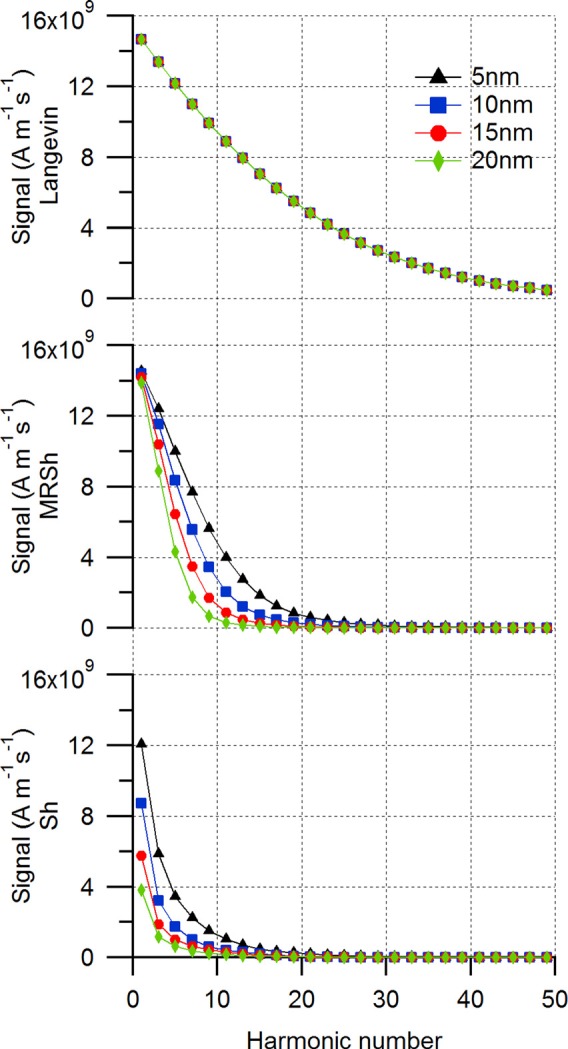
Predicted effect of shell thickness on harmonic spectra according to the Langevin function and the Sh and MRSh equations. For the predictions of the Sh and MRSh equations, as the shell thickness increases, the Brownian relaxation time increases, resulting in lower signal intensity and faster decay in the magnitude of the higher harmonics. In contrast, because the Langevin function neglects the effects of relaxation time, the corresponding harmonic spectra do not change with hydrodynamic diameter. The symbols represent the magnitude of each odd harmonic. The solid lines are used to serve as a guide to the eye.
Next, we consider the case of varying core diameter at a fixed hydrodynamic diameter (70 nm), for which the Brownian relaxation time remains constant, whereas the Langevin parameter varies cubically with respect to core diameter. As seen in Fig. 3, when a 4.5 kHz, 25 mT amplitude field is applied, the spectrum for a core diameter of 50 nm predicted using the Langevin function shows the highest signal and the slowest decay in the harmonics. In contrast, the spectra predicted by the Sh equation show the lowest magnitude in the harmonics. Furthermore, according to the Sh equation, the harmonic spectra for all particles considered would overlap. This is because in the Sh equation, the relaxation time is independent of the magnitude of the Langevin parameter, which parameterizes the relative magnitudes of the applied magnetic field and thermal energy. Finally, the spectra predicted by the MRSh equation show that the signal increases with increasing core diameter. This can be attributed to the decrease in the parallel relaxation time with increasing core diameter, illustrated in Fig. 4, which results in an increase in the rate of change of magnetization and therefore an increase in the magnitude of the harmonics.
FIG. 3.
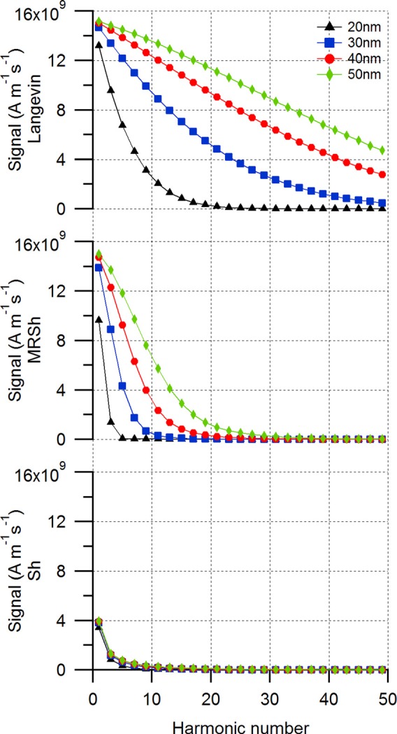
Predicted effect of core diameter on harmonic spectra according to the Langevin function and the Sh and MRSh equations. In the MRSh equation, as the core diameter increases, the parallel relaxation time decreases, resulting in a faster rate of change of magnetization and a correspondingly larger signal.
FIG. 4.
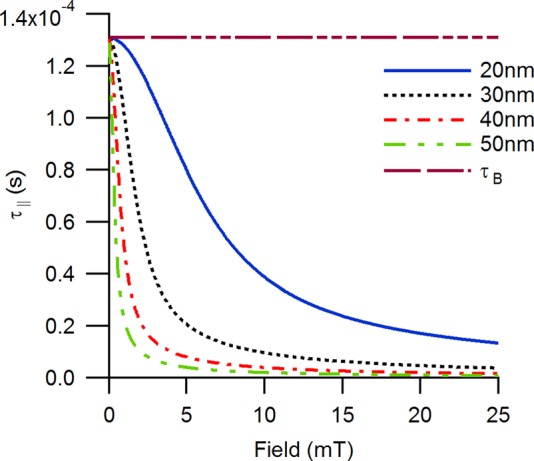
Dependence of the parallel relaxation time in the MRSh equation on the magnitude of the applied magnetic field for various core diameters.
Next, we consider the effect of the frequency of the applied magnetic field on the harmonic spectra. Representative results are presented in Fig. 5. The harmonic spectra predicted by all the models show an increase in the signal with an increase in frequency because for a constant excitation field amplitude, the increase in frequency leads to an increase in the rate at which the field reaches its maximum value and consequently to faster rate of change of magnetization. As the signal is proportional to the rate of change of magnetization, we see an increase in the signal. For the Langevin function, we observe a higher number of harmonics since according to that model, the particles align instantaneously with the alternating magnetic field. In contrast, the Sh and MRSh equations predict that higher harmonics will decay faster as the frequency of the applied alternating magnetic field increases. This is attributed to particles with finite relaxation times being unable to respond to rapidly changing magnetic fields, resulting in a decrease in the magnitude of the peak magnetization of the suspension and therefore in a decrease in the rate of change of magnetization and corresponding signal strength. Interestingly, the harmonics are predicted to decay at a slightly faster rate in the case of the Sh equation, compared to the MRSh equation. This is attributed to the effect of magnetic field amplitude on shortening the relaxation time, which is accounted for solely by the MRSh equation, and leading to a magnetization response that more closely tracks the change in magnetic field.
FIG. 5.
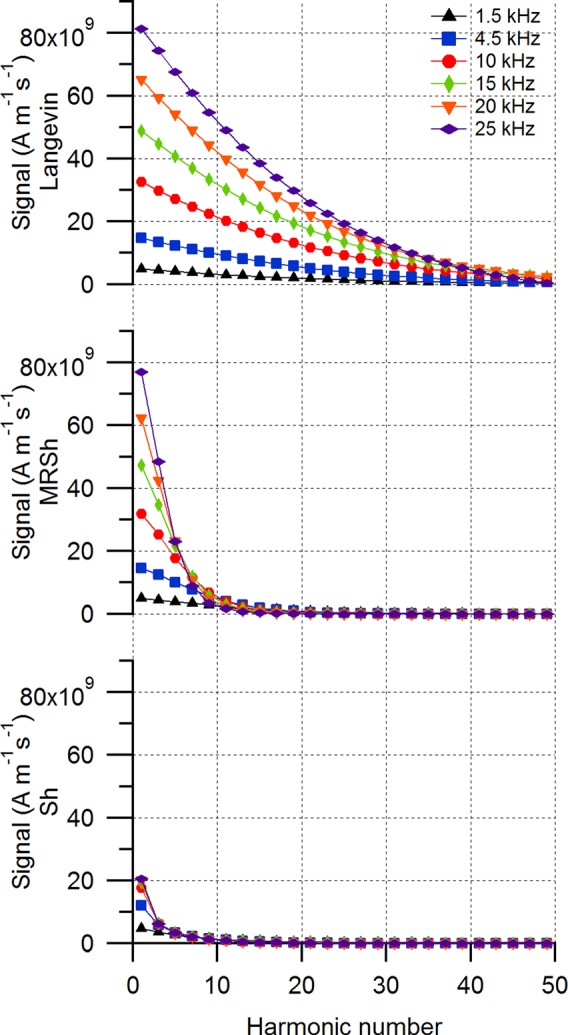
Predicted effect of variation of field frequency on the harmonic spectra according to the Langevin function and the Sh and MRSh equations. The magnetic field amplitude was 25 mT. Particles were modeled as 30 nm core diameter and 5 nm shell thickness.
Finally, we consider the effect of field amplitude on the harmonic spectra, as predicted by the Langevin function and the Sh and MRSh equations. In this case, the field amplitude was varied from 5 mT to 25 mT at a fixed frequency of 1.5 kHz and 25 kHz. Fig. 6 shows that all three models predict an increase in the magnitude of the harmonics with increasing field strength. In all cases, since the field amplitude increases at constant frequency, this leads to an effective increase in the rate at which the field magnitude changes. As the magnetization is dependent on the field magnitude, this results in a greater rate of change of magnetization at constant field frequency, ultimately leading to an increase in signal. This effect is more significant for 25 kHz (Fig. 6(b)) in cases with field dependent relaxation time, modeled using the MRSh equation, where the magnitude of the first harmonic is much more sensitive on the applied field amplitude than that for the predictions of the Langevin function and Sh equation. For the spectra predicted using the Sh equation, not much variation is observed in the signal for variation in field strength as compared to the signal spectra obtained using the Langevin function and the MRSh equation. At higher field strength, the torque exerted on the dipoles by the magnetic field is greater, forcing the particles to align with the field at a faster rate. This increase in torque as well as the increase in net magnetization of the particles leads to an increase in signal. The number of significant harmonics is also higher with an increase in field strength. Also, we can observe from Fig. 4 that the relaxation time decreases with increasing field strength, resulting in a reduction in the delay experienced by the particles in following the alternating field. This physical phenomenon is illustrated in Fig. 1 where it is seen that the magnetization predicted by the MRSh equation shows smaller deviation from the magnetization predicted by the Langevin function as compared to the magnetization predicted by the Sh equation.
FIG. 6.

Predicted effect of the peak amplitude of the applied alternating magnetic field on the harmonic spectra according to the Langevin function and the Sh and MRSh equations. Nanoparticles were modeled as 30 nm core diameter and 5 nm shell thickness. The frequency of the magnetic field was modeled as (a) 1.5 kHz and (b) 25 kHz.
In order to test the predictive power of these models, we compared their predictions to experimentally measured MPS harmonic spectra obtained using a Bruker spectrometer. A suspension of cobalt ferrite nanoparticles with narrow size distribution was used as a model particle system with well-characterized magnetic relaxation mechanism. The volume-weighted hydrodynamic diameter distribution determined from dynamic light scattering measurements, illustrated in Fig. 7(a), was fit to a lognormal size distribution model to obtain a volume-weighted average hydrodynamic diameter of 18 nm and geometric deviation of ln σ = 0.0658. There was evidence of aggregates with volume-weighted diameter of 45–55 nm, most likely due to formation of particle dimers. Transmission electron microscopy imaging of the nanoparticles, illustrated in Fig. 7(b), indicated that the suspension consisted mostly of individual nanoparticles with a number-weighted average physical diameter of 14 nm and geometric deviation of ln σ = 0.122, obtained after fitting the size distribution histogram illustrated in Fig. 7(c) to a lognormal size distribution. The Brownian relaxation of these cobalt ferrite nanoparticles was confirmed through DMS measurements of the particles suspended in toluene, with representative spectra illustrated in Fig. 7(d). It was observed that the in-phase (open circles) and out-of-phase (close circles) components of the dynamic susceptibility crossed at the peak of the out-of-phase susceptibility curve, indicating ideal Brownian behavior described by the Debye model.22 Using the peak frequency and the relation , the hydrodynamic diameter was estimated to be approximately 17 nm, in excellent agreement with that determined using dynamic light scattering.
FIG. 7.

Characterization of cobalt ferrite particles using (a) dynamic light scattering (DLS) and (b) transmission electron microscope (TEM). (c) Distribution of physical diameter of particles found using TEM and (d) dynamic magnetic susceptibility (DMS) measurements confirming presence of particles relaxing by the Brownian mechanism from the peak location.
We used the independently determined physical and magnetic properties of the cobalt ferrite nanoparticles to predict their harmonic spectra according to the three models: the Langevin function and the Sh and MRSh equations. A comparison of the predicted harmonic spectra and those measured using the Bruker MPS is presented in Fig. 8. Because in the Bruker MPS the fundamental harmonic from the nanoparticle response cannot be differentiated from signal generated by the excitation field, the harmonics are presented starting from the 3rd and are normalized with respect to the magnitude of the 3rd harmonic. Of note, all three models predict trends in harmonic spectra that are in excellent qualitative agreement with the experimentally observed trend in change in harmonic spectra up to the 19th harmonic. That is to say, the experiments and simulations all show what appears to be exponential decay of the magnitude of the normalized harmonics. However, quantitatively it is clear that the predictions of the Langevin function show the greatest deviation, while the predictions of the Sh and, to a lesser extent, MRSh equations had excellent quantitative agreement with the experimental harmonic spectra up to the 19th harmonic. This agreement is particularly remarkable because all physical and magnetic properties used in the simulations were independently determined. That is, there were no fitting parameters involved in these comparisons.
FIG. 8.
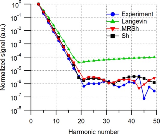
Comparison of model predictions with experiment for cobalt ferrite particles suspended in toluene showing spectra normalized using the magnitude of the 3rd harmonic. The suspension of particles was subjected to a field of frequency 25 kHz and amplitude 25 mT in the Bruker MPS.
Unfortunately, this experiment could not differentiate between the Sh and MRSh models, and therefore shed light on the potential relevance of field-dependent relaxation times on the harmonic spectra of magnetic nanoparticles in MPI. The reason for this shortcoming becomes evident upon reconsidering Figs. 3 and 4, where it can be seen that the effect of field dependent relaxation is expected to be more prominent for larger core diameters. Future experiments are planned to study these effects experimentally. Regardless, the excellent quantitative agreement between the predictions of the Sh and MRSh equations, with no fitting parameters, and the experimentally measured harmonic spectra illustrates the potential value of ferrohydrodynamic modeling in MPI.
V. CONCLUSIONS
The assumption that particles respond instantaneously to the applied field, intrinsic in using the Langevin function, has been recognized as an inaccurate model of the behavior of magnetic nanoparticles used in MPI. This has motivated recent efforts to develop more accurate models that take into account finite relaxation and field-dependence of the magnetic relaxation time. Here, we demonstrated the use of the Sh equation, which accounts for finite magnetic relaxation, and the use of the MRSh equation, which includes the field-dependent relaxation time, to predict the performance of nanoparticles for use in MPS. The number of harmonics contributing significantly to the signal was found to be greater for predictions obtained using the MRSh equation, as compared to the Sh equation, although both predict that the magnitude of the harmonics decays much faster than according to the Langevin function. The study showed how variation in core diameter, coating thickness, excitation field frequency, and field magnitude affect the performance of the nanoparticles in the MPS. Under the assumptions used in the calculations, the models seem to indicate that the use of large core diameter particles with small coating thickness and magnetic fields with high frequency and strength may produce the best signal. Qualitative agreement was observed between the harmonic spectra predicted by the Langevin function and that measured for cobalt ferrite nanoparticles using the Bruker MPS, up to the 19th harmonic, whereas qualitative as well as quantitative agreement was observed between the predictions of the Sh and, to a lesser extent, the MRSh equation and the experimental measurements. These results highlight the potential of ferrohydrodynamic modeling in magnetic particle imaging.
ACKNOWLEDGMENTS
This work was supported by the National Institutes of Health (1R21EB018453-01A1) and the University of Florida. We would like to thank Dr. Nicoleta Baxan at Bruker BioSpin MRI GmbH for testing the particles in the MPS.
References
- 1. Gleich B. and Weizenecker R., Nature 435, 1214 (2005). 10.1038/nature03808 [DOI] [PubMed] [Google Scholar]
- 2. Weizenecker J., Gleich B., Rahmer J., Dahnke H., and Borgert J., Phys. Med. Biol. 54, L1 (2009). 10.1088/0031-9155/54/5/L01 [DOI] [PubMed] [Google Scholar]
- 3. Bulte J. W., Walczak P., Gleich B., Weizenecker J., Markov D. E., Aerts H. C., Boeve H., Borgert J., and Kuhn M., Proc. Soc. Photo-Opt. Instrum. Eng. 7965, 79650z (2011). 10.1117/12.879844 [DOI] [PMC free article] [PubMed] [Google Scholar]
- 4. Borgert J., Schmidt J. D., Schmale I., Rahmer J., Bontus C., Gleich B., David B., Eckart R., Woywode O., Weizenecker J., Schnorr J., Taupitz M., Haegele J., Vogt F. M., and Barkhausen J., J. Cardiovasc. Comput. Tomogr. 6, 149 (2012). 10.1016/j.jcct.2012.04.007 [DOI] [PubMed] [Google Scholar]
- 5. Biederer S., Knopp T., Sattel T. F., Ludtke-Buzug K., Gleich B., Weizenecker J., Borgert J., and Buzug T. M., J. Phys. D: Appl. Phys. 42, 205007 (2009). 10.1088/0022-3727/42/20/205007 [DOI] [PubMed] [Google Scholar]
- 6. Ferguson R. M., Khandhar A. P., and Krishnan K. M., J. Appl. Phys. 111, 07B318 (2012). 10.1063/1.3676053 [DOI] [PMC free article] [PubMed] [Google Scholar]
- 7. Weaver J. B., Rauwerdink A. M., Sullivan C. R., and Baker I., Med. Phys. 35, 1988 (2008). 10.1118/1.2903449 [DOI] [PMC free article] [PubMed] [Google Scholar]
- 8. Weaver J. B. and Kuehlert E., Med. Phys. 39, 2765 (2012). 10.1118/1.3701775 [DOI] [PMC free article] [PubMed] [Google Scholar]
- 9. Rauwerdink A. M. and Weaver J. B., J. Magn. Magn. Mater. 322, 609 (2010). 10.1016/j.jmmm.2009.10.024 [DOI] [Google Scholar]
- 10. Dhavalikar R. and Rinaldi C., J. Appl. Phys. 115, 074308 (2014). 10.1063/1.4866680 [DOI] [Google Scholar]
- 11. Shliomis M. I., Sov. Phys. - JETP 34, 1291 (1972). [Google Scholar]
- 12. Martsenyuk M. A., Raikher Y. L., and Shliomis M. I., Sov. Phys. - JETP 38, 413 (1974). [Google Scholar]
- 13. Park J., An K. J., Hwang Y. S., Park J. G., Noh H. J., Kim J. Y., Park J. H., Hwang N. M., and Hyeon T., Nature Mater. 3, 891 (2004). 10.1038/nmat1251 [DOI] [PubMed] [Google Scholar]
- 14. Rosensweig R., Ferrohydrodynamics ( Dover, New York, 1997). [Google Scholar]
- 15. Goodwill P. W. and Conolly S. M., IEEE Trans. Med. Imaging 29, 1851 (2010). 10.1109/TMI.2010.2052284 [DOI] [PubMed] [Google Scholar]
- 16. Goodwill P. W., Tamrazian A., Croft L. R., Lu C. D., Johnson E. M., Pidaparthi R., Ferguson R. M., Khandhar A. P., Krishnan K. M., and Conolly S. M., Appl. Phys. Lett. 98, 262502 (2011). 10.1063/1.3604009 [DOI] [Google Scholar]
- 17. Croft L. R., Goodwill P. W., and Conolly S. M., IEEE Trans. Med. Imaging 31, 2335 (2012). 10.1109/TMI.2012.2217979 [DOI] [PMC free article] [PubMed] [Google Scholar]
- 18. Shliomis M. I., Phys. Rev. E 64, 060501 (2001). 10.1103/PhysRevE.64.060501 [DOI] [PubMed] [Google Scholar]
- 19. Soto-Aquino D. and Rinaldi C., Phys. Rev. E 82, 046310 (2010). 10.1103/PhysRevE.82.046310 [DOI] [PubMed] [Google Scholar]
- 20. Soto-Aquino D., Rosso D., and Rinaldi C., Phys. Rev. E 84, 056306 (2011). 10.1103/PhysRevE.84.056306 [DOI] [PubMed] [Google Scholar]
- 21. Goodwill P. W., Saritas E. U., Croft L. R., Kim T. N., Krishnan K. M., Schaffer D. V., and Conolly S. M., Adv. Mater. 24, 3870 (2012). 10.1002/adma.201200221 [DOI] [PubMed] [Google Scholar]
- 22. Mazo R. M., Brownian Motion: Fluctuations, Dynamics, and Applications ( Oxford University Press, Inc., New York, 2002). [Google Scholar]