Local dependence in random graph models: characterization, properties and statistical inference

Summary

Dependent phenomena, such as relational, spatial and temporal phenomena, tend to be characterized by local dependence in the sense that units which are close in a well-defined sense are dependent. In contrast with spatial and temporal phenomena, though, relational phenomena tend to lack a natural neighbourhood structure in the sense that it is unknown which units are close and thus dependent. Owing to the challenge of characterizing local dependence and constructing random graph models with local dependence, many conventional exponential family random graph models induce strong dependence and are not amenable to statistical inference. We take first steps to characterize local dependence in random graph models, inspired by the notion of finite neighbourhoods in spatial statistics and M-dependence in time series, and we show that local dependence endows random graph models with desirable properties which make them amenable to statistical inference. We show that random graph models with local dependence satisfy a natural domain consistency condition which every model should satisfy, but conventional exponential family random graph models do not satisfy. In addition, we establish a central limit theorem for random graph models with local dependence, which suggests that random graph models with local dependence are amenable to statistical inference. We discuss how random graph models with local dependence can be constructed by exploiting either observed or unobserved neighbourhood structure. In the absence of observed neighbourhood structure, we take a Bayesian view and express the uncertainty about the neighbourhood structure by specifying a prior on a set of suitable neighbourhood structures. We present simulation results and applications to two real world networks with ‘ground truth’.

1. Introduction

Network data arise in many fields, including biology, the health sciences, economics, political science, sociology, machine learning and engineering. In these fields there are many applications with important societal implications, such as protein–protein interactions, the spread of infectious diseases, contagion in financial markets, insurgencies, terrorist networks, criminal networks, social networks, the Internet and power grids (e.g. Kolaczyk (2009)).

We consider a single observation of a network (e.g. a social network) with n nodes and N = n(n − 1) directed or N = n(n − 1)/2 undirected edge variables. The statistical analysis of a single observation of a network is more challenging than the statistical analysis of multiple independent networks, because such data are both dependent and high dimensional and give rise to unique conceptual, computational and statistical challenges.

We are concerned with problems of specification in the sense of Fisher (1922), page 313, i.e. with the problem of identifying families of distributions which are capable of modelling a wide range of dependences of substantive interest and are amenable to statistical inference. In the past decade, exponential random graph models (ERGMs) have attracted much attention (e.g. Frank and Strauss (1986), Wasserman and Pattison (1996) and Lusher et al. (2013)). Despite attractive finite sample properties (e.g. Barndorff-Nielsen (1978)), ERGMs have turned out to be problematic models of real world networks (e.g. Snijders (2002), Handcock (2003), Hunter et al. (2008) and Chatterjee and Diaconis et al. (2013)).

One of the most striking observations is that some of the most interesting ERGMs do not place much probability mass on graphs which resemble real world networks (e.g. Handcock (2003) and Hunter et al. (2008)). Let Y ∈ 𝕐 be a random graph on a finite set of nodes, corresponding to edge variables Y_i,j between pairs of nodes (i, j). To simplify the discussion, suppose that the edge variables Y_i,j are binary, i.e. Y_i,j ∈ {0, 1}. A convenient representation of a distribution ℙ with support 𝕐 is as an exponential family of the form

$${\mathbb{\mathbb{P}}}_{\theta }(\mathbf{Y}=\mathbf{y})=\exp \{\langle \theta ,s\left(\mathbf{y}\right)\rangle -\psi \left(\theta \right)\},\mathbf{y}\in \mathbb{𝕐},$$ (1)

where ⟨θ, s(y)⟩ denotes the inner product of a d-vector of natural parameters θ and a d-vector of sufficient statistics s(y), and ψ(θ) is a log-normalizing constant. The d-vector of sufficient statistics may include statistics of interest, such as the number of transitive triples of nodes (e.g., in friendship networks, ‘a friend of my friend is my friend’). Such statistics induce dependence between edge variables and are of great interest in the fast growing field of network science (e.g. Wasserman and Faust (1994), Kolaczyk (2009) and Lusher et al. (2013)). If S=s(Y) denotes the vector of sufficient statistics and 𝕊 denotes the convex hull of {s(y):y∈𝕐}, then the induced distribution of S is given by

$${\mathbb{\mathbb{Q}}}_{\theta }(S\in S)={\mathbb{\mathbb{P}}}_{\theta }\{\mathbf{Y}\in S^{-1}\left(S\right)\}=\underset{\mathbf{y}\in S^{-1}\left(S\right)}{\Sigma }{\mathbb{\mathbb{P}}}_{\theta }(\mathbf{Y}=\mathbf{y}),$$ (2)

where S⁻¹(S) denotes the subset of 𝕐 mapping into S ⊂ 𝕊. If the sufficient statistics include counts of the number of transitive triples and other subgraph configurations, then the induced distribution of S tends to place much probability mass on extreme graphs which do not resemble real world networks. There is both theoretical and empirical evidence which suggests that many families of distributions with such count statistics place much mass on the relative boundary rather than in the relative interior of 𝕊 (e.g. Snijders (2002), Handcock (2003) and Hunter et al. (2008)). Worse, theoretical results indicate that the behaviour of conventional ERGMs does not improve as the number of nodes n increases, but deteriorates (Strauss, 1986; Jonasson, 1999; Schweinberger, 2011; Butts, 2011). The best-known examples are Markov random graph models (Frank and Strauss, 1986), though other interesting models are problematic as well. The flawed nature of conventional ERGMs is demonstrated by Fig. 1. It relates to an ERGM of the form (1) with the number of edges and triangles as sufficient statistics with n=100 nodes and N = 4950 undirected edge variables. Fig. 1 shows the prior predictive distributions of the sufficient statistics from the model, which is described in detail in Section 5.1. It demonstrates that the prior predictive distribution places most of its mass on graphs which are extreme in terms of the number of edges and triangles.

Fig. 1.

Prior predictions of the number of (a) edges and (b) triangles under the global triangle model with N = 4950 variables: note the extreme polarization

In this paper, we address the root of the problem by characterizing and constructing well-behaved random graph models which are amenable to statistical inference. The point of departure is the observation that many statistics of interest, S, are sums of random variables, e.g. counts of the number of edges and transitive triples. The distribution of (normed) sums of independent or weakly dependent random variables tends to be Gaussian by virtue of some version of the central limit theorem (e.g. Billingsley (1995)). If the expected value of S is in the relative interior of 𝕊, then the model should place significant mass around the expected value of S by virtue of the approximate Gaussian distribution of S. Therefore, for all expected values of S in the relative interior of 𝕊, the model should place much mass on the relative interior of 𝕊. The difficulty is that, in the absence of spatial, temporal and other structure, it is not evident which edge variables should be dependent. Therefore, the specification of random graph models with weak dependence is challenging and conventional ERGMs induce either no dependence and are simplistic (e.g. Bernoulli random graph models) or strong dependence and are near degenerate (e.g. Markov random graph models; Frank and Strauss (1986)).

We take first steps to characterize local dependence in random graph models in Section 2. We demonstrate that local dependence endows random graph models with desirable properties which make them amenable to statistical inference. One property is a natural domain consistency condition that any probability model should satisfy, but many parameterizations of ERGMs do not satisfy (Shalizi and Rinaldo, 2013). A second and more important property is asymptotic Gaussian behaviour of statistics, which suggests that random graph models with local dependence place much probability mass around the expected value of statistics of interest. We discuss the construction of random graph models with local dependence in Section 3 and Bayesian inference given complete as well as incomplete data in Section 4. If suitable neighbourhood structure is observed, at least two approaches to statistical inference are possible, depending on whether the observed neighbourhood structure is regarded as fixed or random. If no suitable neighbourhood structure is observed, we take a Bayesian view and express the uncertainty about the neighbourhood structure by specifying a prior on a set of suitable neighbourhood structures, using hierarchical parametric and non-parametric priors and auxiliary variable Markov chain Monte Carlo methods. We present simulation results and applications to two real world networks with ground truth in Section 5.

The data that are analysed in the paper and the programs that were used to analyse them can be obtained from http://wileyonlinelibrary.com/journal/rss-datasets

1.1. Other related work

Snijders et al. (2006) and Hunter and Handcock (2006) considered non-linear constraints on the parameter space of ERGMs. Such curved ERGMs have been applied with some success (Hunter et al., 2008) but do not admit simple representations of dependences and the interpretation of parameters is challenging, as noted by Snijders et al. (2006), page 149. An alternative is latent variable models, which we discuss in Section 2.1. Selected special cases and other related work are discussed in Section 3.4.

2. Dependence

We discuss in Section 2.1 two broad approaches to modelling dependence, one based on latent variable models and the other based on ERGMs, and we argue that ERGMs are attractive when dependence is of substantive interest. We discuss in Section 2.2 the challenges that are encountered in modelling dependence of substantive interest by ERGMs. In Section 2.3, we introduce a notion of local dependence and in Section 2.4 we show that that local dependence endows models with desirable properties which make them amenable to statistical inference.

2.1. Dependence of substantive interest

Most relational phenomena are dependent phenomena, and dependence is often of substantive interest. Examples can be found in the social sciences (e.g. Wasserman and Faust (1994) and Lusher et al. (2013)), economics (e.g. Jackson (2008)), the health sciences (e.g. Welch et al. (2011)) and physics (Newman et al., 2002). As an example, if (i, j, k) is a triple of nodes and the edge variables Y_i,j, Y_j,k, Y_i,k ∈ {0, 1} are binary and undirected, then the triple is called transitive if Y_i,j, Y_j,k, Y_i,k = 1, i.e. there are edges between i and j as well as j and k and i and k. Other examples were discussed by Wasserman and Faust (1994) and Lusher et al. (2013).

When modelling transitivity and other dependences, it is not attractive to assume conditional independence of edge variables, e.g.

$$Y_{i,j}\mid p_{i,j}\stackrel{\mathrm{ind}}{~}\mathrm{Bernoulli}\left(p_{i,j}\right),i<j,$$ (3)

where p_i,j denotes the probability of a binary undirected edge between nodes i and j, which may depend on observed and unobserved latent variables. Examples of models of the form (3) are stochastic block models (e.g. Nowicki and Snijders (2001)) and mixed membership models (e.g. Airoldi et al. (2008)), random-effects and mixed effects models (e.g. van Duijn et al. (2004) and Hoff (2005)) and latent space models (Hoff et al., 2002; Schweinberger and Snijders, 2003; Handcock et al., 2007; Krivitsky et al., 2009). Although models of the form (3) can capture transitive closure by introducing latent structure, such models induce dependence indirectly through latent variables rather than directly. In situations where dependence is of substantive interest, scientists tend to prefer models which allow us to specify dependences directly. Examples are the spatial covariance and variogram functions in spatial random-field models (Cressie, 1993), interaction functions in spatial point processes (Møller and Waagepetersen, 2004) and covariance terms in time series (Granger and Morris, 1976). An additional, well-known example is the Ising model in physics (e.g. Georgii (2011)). The Ising model allows the explicit specification of the nature of interactions between particles. Physicists would hesitate to exchange the Ising model for a latent variable model which assumed that particles are independent conditionally on observed structure (e.g. observed locations on a lattice) or unobserved latent structure.

In the realm of networks, Frank and Strauss (1986) and Wasserman and Pattison (1996) introduced exponential family models which resemble the Ising model in physics and lattice models in spatial statistics and which allow the modelling of a wide range of dependences of substantive interest, including transitive closure. Such models have attracted much attention in the social sciences and health sciences and elsewhere, as Lusher et al. (2013) testifies.

2.2. Modelling dependence: challenges

Despite the fact that ERGMs are the natural relatives of well-established models in physics, spatial statistics, machine learning and artificial intelligence, ERGMs lack something that most other areas have: neighbourhood structure. The lack of neighbourhood structure makes modelling dependence challenging.

In spatial statistics (e.g. Cressie (1993) and Stein (1999)) and time series (e.g. Granger and Morris (1976)) and the related work on mixing conditions in probability theory (Billingsley (1995), pages 363–370, and Dedecker et al. (2007)), it is assumed that dependence decreases as the distance between random variables in the spatial or temporal domain increases. Thus, events may be dependent as long as the distance between the locations of the events is small, whereas distant events are almost dependent. In the realm of networks, though, it is not evident what distance between subgraphs means and how the dependence between subgraphs should decrease. A possible approach is to assume uniform weak dependence in the sense that all edges and subgraphs in large graphs are almost independent. Such dependence assumptions are not appealing, however, because network science would expect strong local dependence between some of the edges and subgraphs.

In fact, even when spatial or temporal structure is available, there is often more local structure than would be expected on the basis of the location of nodes in space and time: for example, some subsets of nodes may be close in geographical space, but the members of the subset may be distant in ‘network space’, whereas other subsets of nodes may be distant in geographical space, but close in network space, where network space is understood as other structure that is not captured by geographical space; for example, researchers in the same building, on the same floor and in the same department may not collaborate, but may engage in transitive collaborations with other researchers who are distant in geographical space.

A well-known example of the challenge of modelling dependence is Markov random graph models (Frank and Strauss, 1986). Suppose that the random graph Y is undirected and binary. Motivated by the nearest neighbour definition in physics (Georgii, 2011) and spatial statistics (Besag, 1974), Frank and Strauss (1986) called two dyads {i, j} and {k, l} neighbours if {i, j} and {k, l} share a node and assumed that, if {i, j} and {k, l} are not neighbours, then Y_i,j and Y_k,l are independent conditionally on the rest of random graph Y. Markov random graph models can be represented in exponential family form (1) with the number of edges s₁(y) = Σ_i<j y_i,j, the number of k-stars s_k(y) = Σ_iΣ_j1<…<jk y_i,j1… y_i,jk and the number of triangles $s_n\left(\mathbf{y}\right)={\Sigma }_{i<j<k}{y}_{i,j}{y}_{j,k}{y}_{i,k}$ as sufficient statistics. Markov random graph models and generalizations to ERGMs (Wasserman and Pattison, 1996) allow scientists to model transitive closure and other dependences along with covariate-related similarity, which scientists have long considered to be of great interest (e.g. Wasserman and Faust (1994) and Lusher et al. (2013)). Despite the underlying nearest neighbour assumption and its scientific appeal, however, Markov random graph models are problematic models of real world networks. A simple observation by Strauss (1986) that demonstrates the fundamental flaws of Markov random graph models is that, for any given pair of nodes {i, j}, the number of neighbours is 2(n − 2) and thus increases with the number of nodes n. The large and growing neighbourhoods indicate that Markov random graph models induce increasingly stronger dependence as n increases and are problematic when n is large. This has been confirmed by a growing body of theoretical and empirical results (Strauss, 1986; Jonasson, 1999; Snijders, 2002; Handcock, 2003; Hunter et al., 2008; Rinaldo et al., 2009; Schweinberger, 2011; Butts, 2011; Shalizi and Rinaldo, 2013; Chatterjee and Diaconis, 2013).

2.3. Characterizing local dependence

We take first steps to characterize local dependence, drawing inspiration from two sources: network science and probability theory. On the one hand, network science (e.g. Homans (1950), Wasserman and Faust (1994) and Pattison and Robins (2002)) suggests that interactions in networks are local. On the other hand, weak dependence conditions in probability theory, such as mixing conditions (e.g. Billingsley (1995) and Dedecker et al. (2007)), suggest that dependence should be local to ensure weak dependence and thus desirable behaviour, such as central limit theorems. The study of probability measures on infinite domains in physics (e.g. Georgii (2011)), spatial statistics (e.g. Cressie (1993), section 7.3.1, and Stein (1999), chapter 3) machine learning and artificial intelligence (e.g. Singla and Domingos (2007) and Xiang and Neville (2011)) as well as the notion of M-dependence in time series (e.g. Billingsley (1995), pages 363–370) suggest that each random variable should depend on a finite subset of other random variables. In other words, a natural starting point is to assume that each edge variable depends on a finite subset of other edge variables. We adapt the idea of finite neighbourhoods and M-dependence to random graphs as follows.

Definition 1 (local dependence)

Let Y be a random graph with domain D = N × N and sample space 𝕐, where N is a finite set of nodes. The dependence that is induced by a probability measure ℙ on 𝕐 is called local if there is a partition of the set of nodes A into K ≥ 2 non-empty finite subsets A₁, … , A_K, called neighbourhoods, such that the within- and between-neighbourhood subgraphs Y_k,l with domains A_k × A_l and sample spaces 𝕐_k,l satisfy, for all $y\subseteq \mathbb{𝕐}\mathrm{and}{y}_{k,l}\subseteq {\mathbb{𝕐}}_{k,l}$,

$${\mathbb{\mathbb{P}}}_K(\mathbf{Y}\in y)=\underset{k=1}{\overset{K}{\Pi }}{\mathbb{\mathbb{P}}}_{k,k}({\mathbf{Y}}_{k,k}\in y_{k,k})\underset{l=1}{\overset{k-1}{\Pi }}{\mathbb{\mathbb{P}}}_{k,l}({\mathbf{Y}}_{k,l}\in y_{k,l},{\mathbf{Y}}_{l,k}\in y_{l,k}),$$ (4)

where within-neighbourhood probability measures ℙ_k,k induce dependence within subgraphs Y_k,k, whereas between-neighbourhood probability measures ℙ_k,l induce independence between subgraphs, i.e., for all $y_{k,l}\subseteq {\mathbb{𝕐}}_{k,l},y_{i,k}\subseteq {\mathbb{𝕐}}_{i,k,j},y_{\mathrm{B},i,j}\subseteq {\mathbb{𝕐}}_{\mathrm{B},i,j}\mathrm{and}{y}_{\mathrm{B},j,i}\subseteq {\mathbb{𝕐}}_{\mathrm{B},j,i}$,

$${\mathbb{\mathbb{P}}}_{k,l}({\mathbf{Y}}_{k,l}\in y_{k,l},{\mathbf{Y}}_{l,k}\in y_{l,k})=\underset{i\in A_k,j\in A_l}{\Pi }{\mathbb{\mathbb{P}}}_{\mathrm{B},i,j}(Y_{\mathrm{B},i,j}\in y_{\mathrm{B},i,j},Y_{\mathrm{B},i,j}\in y_{\mathrm{B},j,i}),l<k,$$ (5)

where Y_B,i,j denote between-neighbourhood edge variables corresponding to nodes i and j who are not members of the same neighbourhood.

Thus, local dependence breaks down the dependence of the random graph Y into dependence within subgraphs Y_k,k. The construction of random graph models with local dependence is discussed in Section 3.

The first and foremost advantage of local dependence is that it makes no assumptions about the form and strength of dependence within subgraphs. Scientists are free to incorporate dependences of interest, such as transitive closure within subgraphs. In contrast, conventional ERGMs (e.g. Frank and Strauss (1986)) induce unbounded neighbourhoods and global dependence, as discussed in Section 2.2.

A second advantage is that local dependence endows models with desirable properties, which we discuss in Section 2.4.

2.4. Properties of local dependence

We show that random graphs with local dependence have two natural properties. The first property is a domain consistency property that any probability model should have. The second property is asymptotic Gaussian behaviour of statistics of interest. The two properties help to address both problems of specification and distribution in the sense of Fisher (1922), page 313, by allowing us to model a wide range of dependences within subgraphs and facilitating the derivation of the distributions of estimators and goodness-of-fit statistics.

Since we are considering a single observation of a graph, we follow a domain increasing approach to asymptotics that resembles the domain increasing approach in spatial statistics (e.g. Cressie (1993), section 7.3.1, and Stein (1999), chapter 3). Suppose that the domain of the random graph increases as follows. Let A₁, A₂, … be a sequence of non-empty finite sets of nodes and Y₁, Y₂, … be a sequence of random graphs with increasing domain N₁ × N₁, N₂ × N₂, … , where the set of nodes $N_K={\cup }_{k=1}^K{A}_k$ is the union of the sets of nodes A₁, … , A_K.

The first property is a domain consistency property that should be satisfied by any probability model (e.g. Billingsley (1995), section 36), but which many parameterizations of ERGMs do not satisfy (Shalizi and Rinaldo, 2013).

Theorem 1

Let A₁, A₂, … be a sequence of non-empty, finite sets of nodes and Y₁, Y₂, … be a sequence of random graphs with increasing domain N₁ × N₁, N₂ × N₂, … , where $N_K={\cup }_{k=1}^K{A}_k$. Let Y_K+1/K be the random graph Y_K+1 excluding Y_K, i.e. Y_K+1/K corresponds to the within-neighbourhood subgraph Y_K+1,K+1 and the between-neighbourhood subgraphs Y_k,K+1 and Y_k+1,k, k = 1, …, K; and let 𝕐_K+1/K be the sample space of Y_k+1/K. If a sequence of random graphs Y₁, Y₂, … satisfies local dependence, then it is domain consistent in the sense that, for all K > 0 and y_K ⊆ 𝕐_K,

$${\mathbb{\mathbb{P}}}_K({\mathbf{Y}}_K\in y_K)={\mathbb{\mathbb{P}}}_{K+1}({\mathbf{Y}}_K\in y_K,{\mathbf{Y}}_{K+1∕K}\in {\mathbb{𝕐}}_{K+1∕K}).$$ (6)

In other words, the probability measure ℙ_k of random graph Y_k with domain N_k × N_k can be recovered from the probability measure ℙ_k+1 of random graph Y_k+1 with domain N_k+1 × N_k+1 by marginalizing with respect to Y_k+1/K. It is worth noting that the domain consistency condition that is considered here is weaker than the domain consistency condition that was considered by Shalizi and Rinaldo (2013) and is motivated by the way that the domain of local random graphs increases.

In addition to domain consistency, it is desirable that random graphs with increasing domain satisfy sparsity. A random graph can be called sparse if the expected degrees 𝔼(Σ_j Y_i,j) of nodes i are bounded, suggesting that 𝔼(Y_i,j) → 0 as the number of nodes increases. The importance of sparsity has been recognized by social scientists, computer scientists, mathematicians (e.g. Jonasson (1999) and Lovaász (2012), page viii and page 4) and statisticians (e.g. Krivitsky et al. (2011) and Vu et al. (2013)). Sparsity embodies the notion that, in the real world, resources are bounded—animals and humans face real world constraints such as limited time and therefore cannot maintain arbitrarily many relationships. If random graphs with local dependence do not satisfy sparsity, then the expected degrees of nodes would be dominated by edges to nodes in other neighbourhoods, which would be in conflict with the notion of local interaction in network science. We therefore focus on graphs where within-neighbourhood subgraphs may be dense, but between-neighbourhood subgraphs are sparse.

Definition 2 (sparsity)

Let A₁, A₂, … be a sequence of non-empty, finite sets of nodes and Y₁, Y₂, … be a sequence of random graphs with increasing domain N₁ × N₁, N₂ × N₂, … , where $N_K={\cup }_{k=1}^K{A}_k$. A sequence of random graphs Y₁, Y₂, … satisfying local dependence is called δ sparse if there exist constants A>0 and δ>0 such that

$$\mathbb{𝔼}(\mid Y_{\mathrm{B},i,j}{\mid }^p)\le A{n}^{\delta },p=1,2.$$ (7)

The second, and more important, property is the fact that the asymptotic distribution of statistics of interest is Gaussian, which helps to address problems of estimation and goodness of fit. In practice, most statistics of interest are sums of subgraph configurations. Let $S_K\subseteq {\times }_{i=1}^d{N}_K$ be a subset of the d-dimensional Cartesian product of N_k with itself and $S_K:S_K\mapsto \mathbb{ℝ}$ be a real-valued function with domain S_k, e.g. the number of edges or transitive triples. Such sums of subgraph configurations can be written as

$$S_K=\underset{i\in S_K}{\Sigma }{S}_{K,i},$$ (8)

where $S_{K,i}={\Pi }_{k=1}^q{Y}_{i,a_k,b_k}$ are interactions of q distinct edge variables $Y_{i,a_k,b_k}$, which resemble the interactions in undirected graphical models and related models in physics (e.g. the Ising model) and spatial statistics (e.g. random fields). If, for example, edge variables are binary and $S_K\subseteq N^3$, then S_k,i = Y_a,bY_b,cY_a,c is an indicator of whether the triple of nodes (a, b, c) is transitive. The sum S_k can be decomposed into within- and between-neighbourhood sums W_k and B_k:

$$S_K=W_K+B_K,$$ (9)

where $W_K={\Sigma }_{k=1}^K{W}_{K,k}$ is the total within-neighbourhood sum, composed of the within-neighbourhood sums $W_{K,k}={\Sigma }_{i\in S_K}{1}_{W,k,i}{S}_{K,i}$ in neighbourhoods k, and $B_K={\Sigma }_{i\in S_K}{1}_{B,i}{S}_{K,i}$ is the total between-neighbourhood sum. The indicator function 1_W,k,i is 1 if subgraph configuration i involves nodes in neighbourhood k and neighbourhood k only and is 0 otherwise, whereas 1_B,i is 1 if S_K,i involves nodes of more than one neighbourhood and is 0 otherwise.

It turns out that sequences of local and sparse random graphs with increasing domain are well behaved in the sense of satisfying a central limit theorem for weakly dependent random variables.

Theorem 2

Let A₁, A₂, … be a sequence of non-empty, finite sets of nodes and Y₁, Y₂, …, be a sequence of random graphs with increasing domain N₁ × N₁, N₂ × N₂, …, where $N_K={\cup }_{k=1}^K{A}_k$. Consider sums of the form $S_K={\Sigma }_{i\in S_K}{S}_{K,i}$, where $S_K\subseteq {\times }_{i=1}^d{N}_K$ and $S_{K,i}={\Pi }_{k=1}^q{Y}_{i,a_k,b_k}$. Suppose that the edge variables Y_a,b satisfy uniform boundedness in the sense that there is a constant C >0 such that, for all K >0, a ∈ N_k and b ∈ N_k, $\mathbb{\mathbb{P}}(\mid Y_{a,b}\mid \le C)=1$. Without loss of generality, assume that, for all K>0 and i ∈ S_k, 𝔼(S_K,i) = 0. If the sequence of random graphs Y₁, Y₂, … is local δ > d-sparse and 𝕍(W_K) → ∞ as K → ∞, then

$$\underset{K\to \infty }{\lim }\underset{1\le k\le K}{\max }\mathbb{\mathbb{P}}\{\mid W_{K,k}\mid >\epsilon \sqrt{}\mathbb{𝕍}\left(W_K\right)\}=0$$ (10)

and

$$\frac{S_K}{\sqrt{}\mathbb{𝕍}\left(S_K\right)}\stackrel{\mathrm{d}}{\to }N(0,1)\mathrm{as}K\to \infty ,$$ (11)

where 𝕍(W_K) and 𝕍(S_K) denote the variance of W_k and S_k respectively.

We discuss implications, starting with the most important: theorem 2 respects the desiderata that random graphs be local and sparse and imposes no constraints on the form and shape of within-neighbourhood probability distributions, granting scientists complete freedom to specify arbitrary dependences of interest within neighbourhoods, such as transitive closure. At the same time, local and sparse random graphs tend to be well behaved in the sense that neighbourhoods cannot dominate the whole graph by equation (10) and the distribution of statistics, e.g. the number of transitive triples, tends to be Gaussian by expression (11) provided that the number of neighbourhoods k is large. As a result, random graph models with local dependence can be expected to place much probability mass around the expected values of statistics. If a graph is observed and the method of estimation (e.g. the method of maximum likelihood in exponential families) matches the expected and observed values of selected statistics, then the goodness of fit of the model with respect to the selected statistics can be expected to be acceptable.

Some additional remarks are in order. The uniform boundedness condition covers the most common cases, including the case of binary edge variables Y_i,j ∈ {0, 1}. Multivariate extensions of the central limit theorem may be obtained by the Cramér–Wold theorem (e.g. Billingsley (1995), page 383). If suitable parameterizations of random graph models with local dependence are chosen, then the δ-method can be used to establish asymptotic normality of maximum likelihood estimators and test statistics along the lines of, for example, DasGupta (2008), section 16.3.

3. Model construction and parameterizations

To construct random graph models with local dependence, a suitable neighbourhood structure is needed. In practice, suitable neighbourhood structure may or may not be observed.

Let Z = (Z₁, …, Z_n) be membership indicators, where Z_i is the vector of membership indicators Z_ik of node i, where Z_ik = 1 if node i is a member of neighbourhood A_k and Z_ik = 0 otherwise. Since most network data are discrete, we consider throughout discrete network data and probability densities with respect to counting measure. We assume that the conditional probability mass function (PMF) of a random graph Y given a neighbourhood structure Z = z can be written as

$$\mathbb{\mathbb{P}}(\mathbf{Y}=\mathbf{y}\mid \mathbf{Z}=\mathbf{z})=\underset{k=1}{\overset{K}{\Pi }}\mathbb{\mathbb{P}}({\mathbf{Y}}_{k,k}={\mathbf{y}}_{k,k}\mid \mathbf{Z}=\mathbf{z})\underset{l=1}{\overset{k-1}{\Pi }}\mathbb{\mathbb{P}}({\mathbf{Y}}_{k,l}={\mathbf{y}}_{k,l},{\mathbf{Y}}_{l,k}={\mathbf{y}}_{l,k}\mid \mathbf{Z}=\mathbf{z}),$$ (12)

where between-neighbourhood PMFs can be factorized into dyad-bound PMFs:

$$\mathbb{\mathbb{P}}({\mathbf{Y}}_{k,l}={\mathbf{y}}_{k,l},{\mathbf{Y}}_{l,k}={\mathbf{y}}_{l,k}\mid \mathbf{Z}=\mathbf{z})=\underset{i\in A_k,j\in A_l}{\Pi }\mathbb{\mathbb{P}}(Y_{\mathrm{B},i,j}=y_{\mathrm{B}},i,j,Y_{\mathrm{B},j,i}=y_{\mathrm{B},j,i}\mid \mathbf{Z}=\mathbf{z}),$$ (13)

whereas the within-neighbourhood PMFs are not assumed to be factorizable.

In practice, the question is the source of the neighbourhood structure Z. If suitable neighbourhood structure were observed, then it should be used. We discuss model construction and two approaches to statistical inference given observed neighbourhood structure in Section 3.1. An important practical problem is that in most applications no suitable neighbourhood structure is observed. We discuss model construction and statistical inference in the absence of observed neighbourhood structure in Section 3.2. Parameterizations are discussed in Section 3.3 and selected special cases in Section 3.4.

3.1. Model construction with observed neighbourhoods

Consider the situation where a suitable neighbourhood structure is observed. It is worth noting that the theoretical results of Section 2.4 suggest that, to be suitable, none of the neighbourhoods should dominate the whole graph.

We consider two approaches to statistical inference given observed neighbourhood structure Z = z_obs and assume that the conditional PMF (12) of random graph Y given observed neighbourhood structure Z = z_obs is parameterized by θ.

The first approach regards the observed neighbourhood structure z_obs as fixed and bases statistical inference on the likelihood function

$$L\left(\theta \right)={\mathbb{\mathbb{P}}}_{\theta }(\mathbf{Y}=\mathbf{y}\mid \mathbf{Z}={\mathbf{z}}_{\mathrm{obs}}).$$ (14)

The second approach considers the observed neighbourhood z_obs as the outcome of a random variable Z with a PMF ℙ_π(Z=z_obs) parameterized by π and bases statistical inference on the likelihood function

$$L(\theta ,\pi )={\mathbb{\mathbb{P}}}_{\theta }(\mathbf{Y}=\mathbf{y}\mid \mathbf{Z}={\mathbf{z}}_{\mathrm{obs}}){\mathbb{\mathbb{P}}}_{\pi }(\mathbf{Z}={\mathbf{z}}_{\mathrm{obs}}).$$ (15)

If the two parameter vectors θ and π are variation independent in the sense that the parameter space Ω_θ,π is a product space of the form Ω_θ,π = Ω_θ × Ω_π, where Ω_θ is the parameter space of θ and Ω_π is the parameter space of π, then the likelihood function is given by

$$L(\theta ,\pi )={\mathbb{\mathbb{P}}}_{\theta }(\mathbf{Y}=\mathbf{y}\mid \mathbf{Z}={\mathbf{z}}_{\mathrm{obs}}){\mathbb{\mathbb{P}}}_{\pi }(\mathbf{Z}={\mathbf{z}}_{\mathrm{obs}})=L\left(\theta \right)L\left(\pi \right),$$ (16)

where L(θ) is given by equation (14) and L(π) is given by L(π)=ℙ_π(Z=z_obs). Thus, if the parameters θ and π are variation independent, then the likelihood function factorizes and statistical inference for θ can be based on L(θ). In other words, the two approaches are equivalent as long as the parameters θ and π are variation independent. In general, the random-neighbourhood approach may be more suitable than the fixed neighbourhood approach when it is believed that the neighbourhoods are generated by a stochastic mechanism and that mechanism is itself of interest. The likelihood function L(θ) can be maximized by the maximum likelihood methods of Hunter and Handcock (2006) by using z_obs as a covariate and Bayesian inference can be conducted by using the Bayesian methods of Koskinen et al. (2010) and Caimo and Friel (2011).

There are multiple data structures which could be exploited to construct random graph models with local dependence. Strauss and Ikeda (1990) suggested constructing neighbourhoods by exploiting the categories of categorical covariates; for example the two categories of the categorical covariate gender could be used to form two neighbourhoods, corresponding to females and males. However, many categorical covariates are collected by surveys and have a small number of categories. The theoretical results in Section 2.4 suggest that the number of neighbourhoods should be large and none of the neighbourhoods should dominate the graph, making categorical covariates with a small number of categories problematic when the number of nodes is large. A second approach exploits multilevel structure. In the health sciences and social sciences, many network data have a multilevel structure in the sense that subgraphs are nested in graphs; for example, researchers are located in departments, departments are nested in buildings, and buildings belong to a campus. Such multilevel structure could be exploited to form the neighbourhood structure. A third approach exploits spatial structure provided that it is available, though spatial structure may not capture the whole dependence, as discussed in Section 2.2.

3.2. Model construction without observed neighbourhoods

It is common that no suitable neighbourhood structure is observed. In such cases, we follow a Bayesian approach and express the uncertainty about the neighbourhood structure by a prior on a set of suitable neighbourhood structures. We consider both hierarchical parametric and non-parametric priors.

In principle, statistical inference could be based on the likelihood function

$$L(\theta ,\pi )=\underset{\mathbf{z}\in Z}{\Sigma }{\mathbb{\mathbb{P}}}_{\theta }(\mathbf{Y}=\mathbf{y}\mid \mathbf{Z}=\mathbf{z}){\mathbb{\mathbb{P}}}_{\pi }(\mathbf{Z}=\mathbf{z}),$$ (17)

where Z is the sample space of Z. The difficulty is that Z is either a finite but large set with exp{n log(K)} elements—provided that the number of neighbourhoods k is fixed and known—or a countably infinite set, and in general the sum cannot be computed by complete enumeration. To facilitate statistical inference, we augment the observed data Y by the unobserved data Z and exploit hierarchical parametric and non-parametric priors.

To be specific, assume that

$${\mathbf{Z}}_i\mid {\pi }_1,\dots ,{\pi }_K\stackrel{\mathrm{IID}}{~}\mathrm{multinomial}(1;{\pi }_1,\dots ,{\pi }_K),i=1,\dots ,n,$$ (18)

is the distribution of membership vectors Z₁, …, Z_n. We note that one could incorporate predictors of memberships by using multinomial logit or probit link functions along the lines of Tallberg (2005).

A parametric approach could be based on Dirichlet priors:

$${\pi }_1,\dots ,{\pi }_K~\mathrm{Dirichlet}({\omega }_1,\dots ,{\omega }_K).$$ (19)

A potential problem with Dirichlet priors is that the number of neighbourhoods k must either be known or selected by model selection methods, which is not straightforward. An alternative is to express the uncertainty about k by specifying a prior for k (e.g. Richardson and Green (1997)), which leads to complicated Markov chain Monte Carlo algorithms. We follow a non-parametric approach based on stick breaking priors (Ishwaran and James, 2001), which sidesteps these difficulties. It allows the number of non-empty neighbourhoods a posteriori to be large, while encouraging it a priori to be small. Suppose that there is an infinite number of neighbourhoods and that nodes belong to neighbourhood k = 1, 2, … with probability π_k, k = 1, 2, …, where

$${\pi }_1=V_1,$$ (20)

$${\pi }_k=V_k\underset{j=1}{\overset{k-1}{\Pi }}(1-V_j),k=2,3,\dots ,$$ (21)

where

$$V_k\mid \alpha \stackrel{\mathrm{IID}}{~}\mathrm{beta}(1,\alpha ),k=1,2,\dots .$$ (22)

Here α>0 is a parameter and ${\Sigma }_{k=1}^{\infty }{\pi }_k=1$ with probability 1 (Ishwaran and James, 2001).

3.3. Parameterizations

Exponential parameterizations of the conditional PMF (12) are convenient, though other parameterizations may be used as well.

The dyad-bound between-neighbourhood PMFs can be written as

$${\mathbb{\mathbb{P}}}_{\theta }(Y_{\mathrm{B},i,j}=y_{\mathrm{B},i,j},Y_{\mathrm{B},j,i}=y_{\mathrm{B},j,i}\mid \mathbf{Z}=\mathbf{z})=\exp \{\langle {\theta }_{\mathrm{B}},s_{\mathrm{B},i,j}(y_{\mathrm{B},i,j},y_{\mathrm{B},j,i})\rangle -{\psi }_{\mathrm{B},i,j}\left({\theta }_{\mathrm{B}}\right)\},$$ (23)

where s_{B, i, j}(y_B,i,j, y_B,j,i) is a vector of between-neighbourhood sufficient statistics, θ_B is a vector of between-neighbourhood natural parameters and ψ_{B, i, j} (θ_B) is the between-neighbourhood log-normalizing constant,

$${\psi }_{\mathrm{B},i,j}\left({\theta }_{\mathrm{B}}\right)=\log \left[\sum _{y_{\mathrm{B},i,j}^{\prime }\in {\mathbb{𝕐}}_{\mathrm{B},i,j}}\sum _{y_{\mathrm{B},j,i}^{\prime }\in {\mathbb{𝕐}}_{\mathrm{B},j,i}}\exp \{\langle {\theta }_{\mathrm{B}},s_{\mathrm{B},i,j}(y_{\mathrm{B},i,j}^{\prime },y_{\mathrm{B},j,i}^{\prime })\rangle \}\right].$$ (24)

The between-neighbourhood sufficient statistics s_B,i,j(y_{B, i, j} , s_B,j,i) may be functions of edges y_B,i,j and y_B,j,i and covariates. In the interest of model parsimony, we assume that the between-neighbourhood parameter vector θ_B is constant across dyads.

The within-neighbourhood PMFs can be written as

$${\mathbb{\mathbb{P}}}_{\theta }({\mathbf{Y}}_{k,k}={\mathbf{y}}_{k,k}\mid \mathbf{Z}=\mathbf{z})=\exp \{\langle {\theta }_{\mathrm{W},k},s_{\mathrm{W},k}\left({\mathbf{y}}_{k,k}\right)\rangle -{\psi }_{\mathrm{W},k}\left({\theta }_{\mathrm{W},k}\right)\},$$ (25)

where s_W,k (y_k,k) is a vector of within-neighbourhood sufficient statistics, θ_W,k is a vector of within-neighbourhood natural parameters and ψ_{W, k} (θ_W,k) is the within-neighbourhood log-normalizing constant,

$${\psi }_{\mathrm{W},k}\left({\theta }_{\mathrm{W},k}\right)=\log \left[\sum _{{\mathbf{y}}_{k,k}^{\prime }\in {\mathbb{𝕐}}_{k,k}}\exp \{\langle {\theta }_{\mathrm{W},k},s_{W,k}\left({\mathbf{y}}_{k,k}^{\prime }\right)\rangle \}\right].$$ (26)

The within-neighbourhood sufficient statistics s_W,k (y_k,k) may include interactions, such as the number of triangles within neighbourhood k, which induce dependence within neighbourhoods. In addition, covariates can be used.

The exponential parameterization of the between- and within-neighbourhood PMFs implies that the conditional PMF of Y given Z can be written as

$${\mathbb{\mathbb{P}}}_{\theta }(\mathbf{Y}=\mathbf{y}\mid \mathbf{Z}=\mathbf{z})=\exp \{\langle \eta (\theta ,\mathbf{z}),s\left(\mathbf{y}\right)\rangle -\psi (\theta ,\mathbf{z})\},$$ (27)

where the vector of parameters η(θ, z) is a linear function of the vectors of between- and within-neighbourhood parameters, the vector of sufficient statistics s(y) is a linear function of between- and within-neighbourhood vectors of sufficient statistics and the log-normalizing constant ψ(θ, z) is given by

$$\psi (\theta ,\mathbf{z})=\sum _{k=1}^K\sum _{l=1}^{k-1}\sum _{i\in A_k,j\in A_l}{\psi }_{\mathrm{B},i,j}\left({\theta }_{\mathrm{B}}\right)+\sum _{k=1}^K{\psi }_{\mathrm{W},k}\left({\theta }_{\mathrm{W},k}\right).$$ (28)

The between- and within-neighbourhood parameter vectors θ_B and θ_W,k index exponential families and therefore conjugate priors exist, though direct sampling from the resulting full conditional distributions is infeasible. In the absence of computational advantages, multivariate Gaussian priors are convenient alternatives:

$$\begin{array}{c}\hfill {\theta }_{\mathrm{B}}\mid {\mu }_{\mathrm{B}},{\Sigma }_{\mathrm{B}}^{-1}~\mathrm{MVN}({\mu }_{\mathrm{B}},{\Sigma }_{\mathrm{B}}^{-1}),\hfill \\ \hfill {\theta }_{\mathrm{W},k}\mid {\mu }_{\mathrm{W}},{\Sigma }_{\mathrm{W}}^{-1}\stackrel{\mathrm{IID}}{~}\mathrm{MVN}({\mu }_{\mathrm{W}},{\Sigma }_{\mathrm{W}}^{-1}),k=1,2,\dots ,\hfill \end{array}$$ (29)

where μ_B and μ_W are mean parameter vectors and ${\Sigma }_{\mathrm{B}}^{-1}\mathrm{and}{\Sigma }_{\mathrm{W}}^{-1}$ are precision matrices of suitable order.

To acknowledge the uncertainty about the hyperparameters α, μ_W and ${\Sigma }_{\mathrm{W}}^{-1}$, we assign conjugate gamma, multivariate Gaussian and Wishart hyperpriors to α, μ_W and ${\Sigma }_{\mathrm{W}}^{-1}$ respectively.

3.4. Special cases and related models

Special cases of interest are the block models of Wang and Wong (1987), the stochastic block models of Nowicki and Snijders (2001) and the mixed membership models of Airoldi et al. (2008). These models assume that edge variables are independent conditionally on an observed or unobserved partition of the set of nodes into subsets, which are called blocks and correspond to neighbourhoods. These models satisfy local dependence but do not allow scientists to specify directly the nature of interactions of interest, as discussed in Section 2.1.

The models of Strauss and Ikeda (1990) were discussed in Section 3.1. The usefulness of the models is limited, because neighbourhood structure may either not be observed, in which case the models cannot be used, or neighbourhood structure is observed but is unsuitable in the sense that the observed number of neighbourhoods is small and the number of nodes is large.

Last, the model of Koskinen (2009) does not restrict dependence to blocks and therefore does not satisfy local dependence.

4. Bayesian inference

We focus on Bayesian inference without observed neighbourhood structure, which is the most common and most challenging case. A Bayesian approach must overcome multiple obstacles. The most serious obstacle is the fact that with positive probability one or more neighbourhoods k contains n_k » 5 nodes and thus one or more within-neighbourhood log-normalizing constants, which are log-sums of $\exp \left\{{(}_2^{n_k})\log \left(2\right)\right\}$ terms (see equation (26)), is intractable. To facilitate posterior computations, we approximate the prior and augment the posterior.

We describe the approximation of the prior in Section 4.1, discuss the augmentation of the posterior and sampling from the augmented posterior in Section 4.2, with additional details in the on-line supplements A and B, and address the non-identifiability of within-neighbourhood parameter vectors and membership indicators in supplement C.

4.1. Prior truncation

The stick breaking prior of Section 3.2 can be approximated by a truncated stick breaking prior along the lines of Ishwaran and James (2001), which facilitates posterior computations.

We choose a maximum number of neighbourhoods, which is denoted by K_max. Some general advice concerning the choice of K_max was given by Ishwaran and James (2001). We are here more concerned with the goodness of fit of the model than the approximation of the stick breaking prior and choose K_max in accordance. In practice, we choose K_max by either

• (a) trying out multiple values of K_max and comparing the goodness of fit of the model,

• (b) exploiting on-the-ground knowledge or

• (c) setting K_max =n.

Strategy (a) is motivated by the fact that model estimation is time consuming and the computing time increases with K_max; thus there is an incentive to choose K_max as small as possible. We demonstrate strategies (a) and (b) in Section 5.3.

Given K_max, the membership probabilities $\pi =({\pi }_1,\dots ,{\pi }_{K_{\max }})$ are constructed by truncated stick breaking (Ishwaran and James, 2001):

$${\pi }_1=V_1,$$ (30)

$${\pi }_k=V_k\underset{j=1}{\overset{k-1}{\pi }}(1-V_j),k=2,\dots ,K_{\max },$$ (31)

where

$$\begin{array}{c}\hfill V_k\mid \alpha \stackrel{\mathrm{IID}}{~}\mathrm{beta}(1,\alpha ),k=1,\dots ,K_{\max }-1,\hfill \\ \hfill V_{K_{\max }}=1,\hfill \end{array}$$ (32)

where α > 0 is a parameter and $V_{K_{\max }}=1$ ensures that ${\Sigma }_{k=1}^{K_{\max }}{\pi }_k=1$. The truncated stick breaking construction of π implies that π is generalized Dirichlet distributed, which is conjugate to multinomial sampling (Ishwaran and James, 2001).

4.2. Posterior augmentation

Under the truncated prior that was described in Section 4.1, the posterior is of the form

$$p(\alpha ,{\mu }_{\mathrm{W}},{\Sigma }_{\mathrm{W}}^{-1},\pi ,{\theta }_{\mathrm{B}},{\theta }_{\mathrm{W}},\mathrm{z}\mid y)\propto p(\alpha ,{\mu }_{\mathrm{W}},{\Sigma }_{\mathrm{W}}^{-1},\pi ,{\theta }_{\mathrm{B}},{\theta }_{\mathrm{W}}){\mathbb{\mathbb{P}}}_{\pi }(\mathbf{Z}=\mathbf{z}){\mathbb{\mathbb{P}}}_{\theta }(\mathrm{Y}=\mathbf{y}\mid \mathbf{Z}=\mathbf{z}),$$ (33)

where the truncated prior is of the form

$$p(\alpha ,{\mu }_{\mathrm{W}},{\Sigma }_{\mathrm{W}}^{-1},\pi ,{\theta }_{\mathrm{B}},{\theta }_{\mathrm{W}})=p\left(\alpha \right)p\left({\mu }_{\mathrm{W}}\right)p\left({\Sigma }_{\mathrm{W}}^{-1}\right)p(\pi \mid \alpha )p\left({\theta }_{\mathrm{B}}\right)\underset{k=1}{\overset{K_{\max }}{\Pi }}p({\theta }_{\mathrm{W},k}\mid {\mu }_{\mathrm{W}},{\Sigma }_{\mathrm{W}}^{-1}),$$ (34)

where ${\theta }_{\mathrm{W}}=({\theta }_{\mathrm{W},1},\dots ,{\theta }_{\mathrm{W},K_{\max }})$ denotes the within-neighbourhood parameter vectors.

Owing to the fact that the conditional PMF of Y is not, in general, tractable, the posterior is doubly intractable, implying that standard Markov chain Monte Carlo methods (e.g. Metropolis–Hastings algorithms) cannot be used to sample from the posterior. Auxiliary variable Markov chain Monte Carlo methods for sampling from doubly intractable posteriors arising in complete-data problems were introduced by Møller et al. (2006) and extended by Murray et al. (2006) and Liang (2010); they have been adapted to networks by Koskinen et al. (2010), Caimo and Friel (2011) and Wang and Atchade (2014). We extend them from the complete-data problems that were considered there to the incomplete-data problem that is considered here.

To facilitate posterior computations, we augment $\alpha ,{\mu }_{\mathrm{W}},{\Sigma }_{\mathrm{W}}^{-1},\pi ,{\theta }_{\mathrm{B}},{\theta }_{\mathrm{W}},\mathbf{Z}\mathrm{and}\mathbf{Y}$ by auxiliary variables ${\theta }_{\mathrm{W}}^{\ast },{\mathbf{Z}}^{\ast }\mathrm{and}{\mathbf{Y}}^{\ast }$. The auxiliary variable Y* can be interpreted as an auxiliary random graph, Z* can be interpreted as an auxiliary neighbourhood structure and ${\theta }_{\mathrm{W}}^{\ast }$ can be interpreted as auxiliary within-neighbourhood parameter vectors. We assume that the joint distribution of $\alpha ,{\mu }_{\mathrm{W}},{\Sigma }_{\mathrm{W}}^{-1},\pi ,{\theta }_{\mathrm{B}},{\theta }_{\mathrm{W}},\mathbf{Z},\mathbf{Y},{\theta }_{\mathrm{W}}^{\ast },{\mathbf{Z}}^{\ast }\mathrm{and}{\mathbf{Y}}^{\ast }$ is of the form

$$\begin{array}{cc}\hfill p(\alpha ,{\mu }_{\mathrm{W}},{\Sigma }_{\mathrm{W}}^{-1},\pi ,{\theta }_{\mathrm{B}},{\theta }_{\mathrm{W}},\mathbf{z},\mathbf{y},{\theta }_{\mathrm{W}}^{\ast },{\mathbf{z}}^{\ast },{\mathbf{y}}^{\ast })& =p(\alpha ,{\mu }_{\mathrm{W}},{\Sigma }_{\mathrm{W}}^{-1},\pi ,{\theta }_{\mathrm{B}},{\theta }_{\mathrm{W}}){\mathbb{\mathbb{P}}}_{\pi }(\mathbf{Z}=\mathbf{z}){\mathbb{\mathbb{P}}}_{\theta }(\mathbf{Y}=\mathbf{y}\mid \mathbf{Z}=\mathbf{z})\hfill \\ \hfill & \times q({\theta }_{\mathrm{W}}^{\ast },{\mathbf{z}}^{\ast }\mid \pi ,{\theta }_{\mathrm{B}},{\theta }_{\mathrm{W}},\mathbf{z},\mathbf{y}){\mathbb{\mathbb{P}}}_{{\theta }^{\ast }}({\mathbf{Y}}^{\ast }={\mathbf{y}}^{\ast }\mid {\mathbf{Z}}^{\ast }={\mathbf{z}}^{\ast }),\hfill \end{array}$$ (35)

where $q({\theta }_{\mathrm{W}}^{\ast },{\mathbf{z}}^{\ast }\mid \pi ,{\theta }_{\mathrm{B}},{\theta }_{\mathrm{W}},\mathbf{z},y)$ is a suitable auxiliary distribution, the conditional distributions Y and Y* belong to the same exponential family of distributions and ${\theta }^{\ast }=({\theta }_B,{\theta }_{\mathrm{W}}^{\ast })$. The augmented posterior is of the form

$$p(\alpha ,{\mu }_{\mathrm{W}},{\Sigma }_{\mathrm{W}}^{-1},\pi ,{\theta }_{\mathrm{B}},{\theta }_{\mathrm{W}},\mathbf{z},{\theta }_{\mathrm{W}}^{\ast },{\mathbf{z}}^{\ast },{\mathbf{y}}^{\ast }\mid \mathbf{y})\propto p(\alpha ,{\mu }_{\mathrm{W}},{\Sigma }_{\mathrm{W}}^{-1},\pi ,{\theta }_{\mathrm{B}},{\theta }_{\mathrm{W}},\mathbf{z},\mathbf{y},{\theta }_{\mathrm{W}}^{\ast },{\mathbf{z}}^{\ast },{\mathbf{y}}^{\ast }).$$ (36)

Integrating out the auxiliary variables ${\theta }_{\mathrm{W}}^{\ast }$, Z* and Y* results in the posterior of α, μ_W , ${\Sigma }_{\mathrm{W}}^{-1}$, π, θ_B, θ_W and Z. Whereas sampling from the posterior (33) is infeasible, sampling from the augmented posterior (36) and integrating out the auxiliary variables ${\theta }_{\mathrm{W}}^{\ast }$, Z* and Y* turns out to be feasible. We discuss Markov chain Monte Carlo steps and improved Markov chain Monte Carlo sampling through variational methods in the on-line supplement.

5. Assessment of local and global models of transitive closure

We compare random graph models with local and global dependence by comparing

• (a) prior predictions of graphs to assess whether models can produce data that resemble real world networks (Section 5.1),

• (b) sampling distributions of Bayesian point and interval estimators (Section 5.2) and

• (c) posterior predictions of graphs to assess whether models make sense in the light of observed data (Section 5.3).

We consider undirected, binary edge variables, i.e. Y_i,j ∈ {0, 1} and Y_i,j = Y_j,i with probability 1, and random graph models capturing transitive closure, because it is one of the most fundamental and problematic forms of dependence. A well-known random graph capturing transitive closure is the triangle model, which is an ERGM of the form (1) with the number of edges y_i,j and triangles y_i,j y_j,hy_i,h as sufficient statistics (Jonasson, 1999; Handcock et al., 2008). Its natural relative is the random graph model of the form (23) and (25), where the between-neighbourhood sufficient statistics are the edges y_i,j between nodes i and j in neighbourhoods k and l, and the within-neighbourhood sufficient statistics are the number of edges y_i,j and triangles y_i,j y_j,hy_i,h within neighbourhoods k. We refer to the two models as the global and local triangle model. The name global triangle model is motivated by the fact that the model is a special case of a Markov random graph model with unbounded neighbourhoods—as explained in Section 2.2—and therefore does not satisfy local dependence.

5.1. Comparison of local and global models of transitive closure

In this subsection, we assess whether models are realistic by considering the prior predictive distributions of the statistics. As discussed in Section 1, the global triangle model places much probability mass on the relative boundary of the convex hull of {s(y) : y ∈ 𝕐}. As networks with extreme values on network statistics may be considered odd, one approach to assessing the realism of a model is to consider the distribution of the statistics that it produces.

The prior predictive distribution under the global triangle model can be written as

$$\mathbb{\mathbb{P}}(\mathbf{Y}=\mathbf{y})=\int p\left(\theta \right){\mathbb{\mathbb{P}}}_{\theta }(\mathbf{Y}=\mathbf{y})\mathrm{d}\theta ,$$ (37)

where p(θ) denotes the prior. On the basis of experience, values of θ₁ outside (−5, 0) and values of θ₂ outside (0, 5) index near-degenerate distributions. Therefore, we choose independent, uniform priors given by θ₁ ~ uniform(5, 0) and θ₂ ~ uniform(0, 5).

The prior predictive distribution under the local triangle model can be written as

$$\begin{array}{cc}\hfill \mathbb{\mathbb{P}}(\mathbf{Y}=\mathbf{y})& =\int \dots \int \sum _{\mathbf{z}\in Z}p(\alpha ,{\mu }_{\mathrm{W}},{\Sigma }_{\mathrm{W}}^{-1},\pi ,{\theta }_{\mathrm{B}},{\theta }_{\mathrm{W}})\hfill \\ \hfill & \times {\mathbb{\mathbb{P}}}_{\pi }(\mathbf{Z}=\mathbf{z}){\mathbb{\mathbb{P}}}_{\theta }(\mathbf{Y}=\mathbf{y}\mid \mathbf{Z}=\mathbf{z})\mathrm{d}\propto \mathrm{d}{\mu }_{\mathrm{W}}\mathrm{d}{\Sigma }_{\mathrm{W}}^{-1}\mathrm{d}\pi \mathrm{d}{\theta }_{\mathrm{B}}\mathrm{d}{\theta }_{\mathrm{W}},\hfill \end{array}$$ (38)

where $p(\alpha ,{\mu }_{\mathrm{W}},{\Sigma }_{\mathrm{W}}^{-1},\pi ,{\theta }_{\mathrm{B}},{\theta }_{\mathrm{W}})$ denotes the prior. We assign independent Gaussian priors with means −1 and 1 and standard deviations 0.25 and 0.25 to within-neighbourhood parameters θ_W,k,1 and θ_W,k,2 respectively. The marginal priors of θ_W,k,1 and θ_W,k,2 ensure that most of the prior probability mass of θ_W,k,1 is concentrated on (−2, 0) and most of the prior probability mass of θ_W,k,2 is concentrated on (0, 2), which cover the most reasonable value of θ_W,k,1 and θ_W,k,2 respectively. To respect the sparse nature of graphs, we assume that the between-neighbourhood parameter θ_B is governed by a Gaussian prior with mean μ_B and standard deviation 1, where the Gaussian prior is centred at μ_B = 3/(n − 1), the value of θ_B under which the expected number of edges of nodes between neighbourhoods is at most 3. The prior of π is given by the Dirichlet(10, … , 10) prior.

We generated 1000 model predictions from the local triangle model with k = 150 neighbourhoods, n = 1000 nodes, and N = 499500 edge variables and 1000 realizations from the global triangle model with n = 100 nodes and N = 4950 edge variables; the difference in the size of the graphs is because the fiawed nature of the global triangle model makes it infeasible to sample much larger graphs than N = 4950. Monte Carlo samples of size 1000 were generated from the prior and, for every one of the draws from the prior, a prediction was generated by a Markov chain of length 10 million for the local triangle model and 100000 for the global triangle model, accepting the final draw of the Markov chain as a draw from the prior predictive distribution; the sample size is proportional to the size of the graphs.

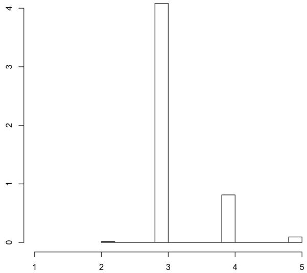
Fig. 1 shows prior predictions of the number of edges and triangles under the global triangle model. The bulk of the prior predictive mass is placed on extreme graphs with few edges and triangles and graphs with almost all possible edges and triangles. We note that the behaviour of the global triangle model tends to deteriorate as the size of the graph increases, as discussed in Section 1. In contrast, Fig. 2 demonstrates that random graph models with local dependence place much prior predictive mass around the mean and all of its mass on graphs which resemble real world networks, i.e. graphs where the average number of edges of nodes ranges from 4 to 6 and where the number of triangles is a small multiple of the number of edges. It is worth repeating that the number of edge variables is 499500, which demonstrates that random graph models with local dependence are well behaved when the number of edge variables is large, in sharp contrast with conventional ERGMs.

Fig. 2.

Prior predictions of the number of (a) edges and (b) triangles under the local triangle model with parametric prior and K = 150 neighbourhoods and N = 499500 edge variables: most prior predictive mass is concentrated around the means of the prior predictions (|)

In short, the model predictions confirm what the theoretical results of Section 2.4 suggested: in contrast with conventional ERGMs, random graph models with local dependence are capable of generating graphs which resemble real world networks and can thus be recommended a priori as models of real world networks.

5.2. Sampling distributions of Bayesian point and interval estimators

We shed light on the frequentist properties of estimators by simulation. We focus on random graph models with local dependence, because fiawed models of the form (1) generate many graphs which fall onto the relative boundary of the convex hull of {s(y) : y ∈ 𝕐} and make statistical inference problematic (e.g. Barndorff-Nielsen (1978), page 151, Handcock (2003), Rinaldo et al. (2009), Koskinen et al. (2010) and Bhamidi et al. (2011)).

Here, we focus on the frequentist properties of posterior point estimators and interval estimators of the local triangle model with K = 7 neighbourhoods, n = 50 nodes and N = 1225 edge variables. We generated 1000 graphs from the local triangle model by using the same prior as used in Section 5.1. To infer from the simulated graphs to the data-generating values of the parameters, we used two priors: a parametric Dirichlet(α, … , α) prior for π with K = 7 with a gamma(1, 0.1) hyperprior for α, and a non-parametric truncated stick breaking prior with K_max = 7 with a gamma(1, 0.1) hyperprior for α. In both cases, the marginal priors of θ_W,1, θ_W,2 and θ_B are independently N(0, 100). We construct 1000 Markov chains with 100000 iterations, discarding the first 20000 iterations as burn-in and recording every 10th post-burn-in iterations.

In practice, within-neighbourhood parameters are of primary interest, because it is the within-neighbourhood models which capture the dependences of interest. Here, we focus on the within-neighbourhood means μ_W,1 and μ_W,2. The sampling distributions of posterior point estimators for μ_W,1 and μ_W,2 under parametric and non-parametric priors are shown in Figs 3 and 4. Despite the small number of neighbourhoods K = 7, the data-generating parameter of the Gaussian mean μ_W of the K = 7 within-neighbourhood parameters θ_W,1, … , θ_W,7 can be recovered in the sense that the posterior median clusters around the data-generating parameter value. The distributions are somewhat asymmetric, which is not surprising considering the small number of K = 7 neighbourhoods. Table 1 shows that interval estimators, e.g. 95% posterior credibility intervals, have acceptable coverage properties, considering the small number of K = 7 neighbourhoods.

Fig. 3.

Sampling distributions of posterior medians of within-neighborhood means (a) μ_W,1 and (b) μ_W,2 under the local triangle model with parametric prior and K = 7 neighbourhoods and N = 1225 edge variables (|, data-generating values): despite the small number of K = 7 neighbourhoods, the data-generating values of the Gaussian mean μ_W of the K = 7 within-neighbourhood parameters θ_W,1,… , θ_W,7 can be recovered

Fig. 4.

Sampling distributions of posterior medians of within-neighbourhood means (a) μ_W,1 and (b) μ_W,2 under the local triangle model with non-parametric prior and K_max = 7 neighbourhoods and N = 1225 edge variables (|, data-generating values): despite the small number of neighbourhoods K_max = 7, the data-generating values of the Gaussian mean μ_W of the K_max = 7 within-neighbourhood parameters θ_W,1,…, θ_W,7 can be recovered

Table 1.

Frequentist properties of posterior medians and 95% posterior credibility intervals of within-neighbourhood means μ_{W ,1} and μ_W,2^†

Prior	Parameter	0.025- quantile	0.50- quantile	0.975- quantile	Coverage (%)
Parametric	μW ,1 =−1	−5.75	−1.48	0.48	86
Parametric	μW,2 =1	0.69	1.26	2.27	98
Non-parametric	μW,1 =−1	−4.19	−1.25	0.26	95
Non-parametric	μW,2 =1	0.26	0.86	1.68	>99

^†Despite the small number of K_max =7 neighbourhoods, the data-generating values of the Gaussian mean μ_W of the K_max =7 within-neighbourhood parameters θ_W,1,… ,θ_W,7 can be recovered.

The results also suggest that the non-parametric approach seems to outperform the parametric approach, at least in terms of coverage for μ_W,1. In addition, we found in the applications in Section 5.3 that the hierarchical non-parametric prior is not overly sensitive to the choice of the hyperparameters of the priors, whereas the hierarchical parametric prior sometimes is sensitive to the choice of hyperparameters, and more so when the specified number of neighbourhoods exceeds the true number of neighbourhoods. Thus, the non-parametric approach seems to have advantages over the parametric approach.

5.3. Application to a terrorist network and a social network

A natural approach to comparing ERGMs and random graph models with local dependence is based on their predictions about observable quantities. Hunter et al. (2008) argued that, in practice, it is imperative to generate model predictions to assess the goodness of fit of network models.

In this section, we compare ERGMs and random graph models with local dependence in terms of posterior predictions in two real world networks with ground truth: the terrorist network behind the Bali bombing in 2002 as well as social relationships among novices within a novitiate.

The posterior predictive distribution under the global triangle model given data y can be written as

$$\mathbb{\mathbb{P}}(\stackrel{.}{\mathbf{Y}}=\stackrel{.}{\mathbf{y}}\mid \mathbf{Y}=\mathbf{y})=\int p(\theta \mid \mathbf{y}){\mathbb{\mathbb{P}}}_{\theta }(\stackrel{.}{\mathbf{Y}}=\stackrel{.}{\mathbf{y}})\mathrm{d}\theta ,$$ (39)

where p(θ|y) denotes the posterior. The posterior predictive distribution under the local triangle model can be written as

$$\begin{array}{cc}\hfill \mathbb{\mathbb{P}}(\stackrel{.}{\mathbf{Y}}=\stackrel{.}{\mathbf{y}}\mid \mathbf{Y}=\mathbf{y})& =\int \dots \int \sum _{\mathbf{z}\in Z}p(\alpha ,{\mu }_{\mathrm{W}},{\Sigma }_{\mathrm{W}}^{-1},\pi ,{\theta }_{\mathrm{B}},{\theta }_{\mathrm{W}},\mathbf{z}\mid \mathbf{y})\hfill \\ \hfill & \times {\mathbb{\mathbb{P}}}_{\theta }(\stackrel{.}{\mathbf{Y}}=\stackrel{.}{\mathbf{y}}\mid \mathbf{Z}=\mathbf{z})\mathrm{d}\propto \mathrm{d}{\mu }_{\mathrm{W}}\mathrm{d}{\Sigma }_{\mathrm{W}}^{-1}\mathrm{d}\pi \mathrm{d}{\theta }_{\mathrm{B}}\mathrm{d}{\theta }_{\mathrm{W}},\hfill \end{array}$$ (40)

where $p(\alpha ,{\mu }_{\mathrm{W}},{\Sigma }_{\mathrm{W}}^{-1},\pi ,{\theta }_{\mathrm{B}},{\theta }_{\mathrm{W}},\mathbf{z}\mid \mathbf{y})$ denotes the posterior. Independent priors θ_i ~ N(0, 25) are used in the case of the ERGM and independent priors α ~ gamma(1, 1), μ_W,i ~ N(0, 1) and ${\sigma }_{\mathrm{W},i}^{-2}$ ~ gamma(10, 10) in the case of the random graph model with local dependence. 120000 draws from the posterior predictive distribution of the ERGM were generated by the Markov chain Monte Carlo algorithm of Caimo and Friel (2011), with a burn-in of 20000 and saving every 10th post-burn-in draw, and 1200000 draws from the posterior predictive distribution of the random graph model with local dependence were generated by the Markov chain Monte Carlo algorithm of Section 4, with a burn-in of 200000 and saving every 100th post-burn-in draw.

5.3.1. Terrorist network behind Bali bombing in 2002

The structure of terrorist networks is of interest with a view to understanding how terrorists communicate, to identify cells (i.e. subsets of terrorists), to isolate cells and to dismantle them. We consider here the network of terrorists behind the Bali, Indonesia, bombing in 2002, killing 202 (Koschade, 2006). The 17 terrorists who carried out the bombing were members of the south-east Asian al-Qaeda affiliate Jemaah Islamiyah. The terrorist network can be represented by a graph with n = 17 nodes and N = 136 edge variables, where Y_i,j = 1 if terrorists i and j were in contact before the bombing and Y_i,j = 0 otherwise. The terrorist network is shown in Fig. 5.

Fig. 5.

Terrorist network behind the Bali bombing in 2002 with N = 136 edge variables: the shaded pie charts represent posterior membership probabilities; the clustering is a by-product of model estimation and is of secondary interest, but it is comforting that it is consistent with ground truth

We start by determining the maximum number of neighbourhoods K_max to truncate the prior. Using strategy (a) described in Section 4.1, we compare the local triangle model with K_max = 2, 3, 4, 5 neighbourhoods in terms of predictive power. Predictive power is taken to be the root-mean-square deviation of the predicted number of triangles. According to Fig. 6(a), the local triangle model with K_max = 2 neighbourhoods is far superior to the global triangle model, which corresponds to K_max = 1 neighbourhood. The local triangle model with K_max = 3 in turn is superior to the local triangle model with K_max = 2, but increasing K_max from 3 to 5 does not increase the predictive power much. Fig. 6(b) compares the local triangle model with stochastic block models. The stochastic block model that is used here is a special case of the local triangle model where the within-neighbourhood sufficient statistics are reduced to the number of edges, which induces conditional independence of edges within neighbourhoods. Stochastic block models are special cases of random graph models with local dependence and not appealing when dependence is of substantive interest, because they assume conditional independence within neighbourhoods, as discussed in Sections 2.1 and 3.4. Fig. 6(b) demonstrates that the stochastic block model has much lower predictive power than the local triangle model.

Fig. 6.

Terrorist network: root-mean-square deviation of the number of triangles plotted against K_max = 2, 3, 4, 5 neighbourhoods: (a) the global triangle model with K_max = 1 is far inferior to the local triangle model with K = 2, 3, 4, 5 neighbourhoods; (b) the stochastic block model (—1—) is likewise far inferior to the local triangle model (—2—)

We compare the global and local triangle model with up to K_max = 5 neighbourhoods in terms of the posterior predictive distribution of the number of edges and triangles, shown in Figs 7 and 8. Under the global triangle model, the posterior predictive distribution is bimodal. In contrast, the posterior predictive distribution under the local triangle model is unimodal and places most mass on graphs which are close to the observed graph in terms of the number of edges and triangles. The fact that the global triangle model places so much mass on dense graphs with almost all edges and triangles indicates that the global triangle model fits much worse than the random graph model with local dependence, no matter which goodness-of-fit statistics are chosen, because the topology of graphs which are local in nature—such as the observed graph—stands in sharp contrast with the topology of dense graphs in terms of connectivity, centrality, transitivity and other interesting features of graphs (e.g. Kolaczyk (2009)). We note that, although other statistics may be used to compare the two models in terms of goodness of fit, the choice of goodness-of-fit statistics here presents compelling evidence.

Fig. 7.

Terrorist network: posterior predictions of the number of (a) edges and (b) triangles under the global triangle model (|, observed numbers): although the number of edge variables N = 136 is not large, the polarization is evident

Fig. 8.

Terrorist network: posterior predictions of the number of (a) edges and (b) triangles under the local triangle model (|, observed numbers): the posterior predictive distributions are unimodal and short tailed, in contrast with Fig. 7

The posterior of α, μ_W,1 and μ_W,2 is shown in Table 2. The mean parameters μ_W,1 and μ_{W, 2} governing the within-neighbourhood parameters tend to be both positive—and more so the mean parameter μ_W,2 governing the within-neighbourhood triangle parameters—which is not surprising in the light of the large number of edges and triangles within neighbourhoods.

Table 2.

Terrorist network: posterior of parameters α, μ_W,1 and μ_W,2

Parameter	0.05- quantile	0.50- quantile	0.95- quantile	Odds of parameter being positive
α	0.36	1.32	3.43	∞
μ W,1	−1.03	0.45	2.00	2.22
μ W,2	−0.27	0.91	2.22	8.74

Last, although the primary purpose of introducing neighbourhoods is the desire to address the model degeneracy and striking lack of fit of ERGMs, predictions of the memberships to neighbourhoods may be of interest as well, e.g. to identify cells. The pie charts in Fig. 5 represent the posterior membership probabilities that were reported by the stochastic relabelling algorithm that is described in the on-line supplement C. The five white-coloured terrorists turn out to be the five members of the so-called support group, which was to supposed to support the so-called main group consisting of all other terrorists. The members of the main group tend to be black coloured, with the exception of Amrozi and Mubarok who are more bright coloured than black coloured. Indeed, although Amrozi and Mubarok belonged to the main group, both resided elsewhere and were almost isolated from the rest of the main group (Koschade, 2006). Most interesting is the membership of Feri. He was a member of the main group and was the suicide bomber who initiated the attack. Feri arrived 2 days before the attack, whereas all other members of the main group had arrived days or weeks earlier and in fact started to leave the night that Feri arrived (Koschade, 2006). As a result, Feri had limited opportunities to communicate with others. In particular, Feri was the one and only member of the main group who did not communicate with the three commanders Muklas (the Jemaah Islamiyah head of operations in Singapore and Malaysia), Samudra (the field commander) and Idris (the logistics commander) (Koschade, 2006). Therefore, the network position of Feri is unique and the uncertainty about his membership is reflected in the posterior membership probability distribution.

In conclusion, random graph models with local dependence capture simple and interesting features of the terrorist network and, under the parameterization that is considered here, posterior membership predictions are consistent with on-the-ground knowledge of the terrorist network.

5.3.2. Social relationships within a novitiate

Sampson (1968) studied social relationships between a group of novices who were preparing to enter a monastic order. The network is a classic data set in social network analysis (White et al., 1976; Handcock et al., 2007) and corresponds to N = 306 relationships between the n = 18 novices measured at three time points spread out over a 12-month period. We consider here the following directed edge variables Y_i,j: if novice i liked novice j at any of the three time points, then Y_i,j = 1; otherwise Y_i,j = 0. The network is plotted in Fig. 9.

Fig. 9.

Sampson network with N = 306 edge variables: the shaded pie charts represent posterior membership probabilities; the clustering is a by-product of model estimation and is of secondary interest, but it is comforting that it is consistent with ground truth

A natural extension of the triangle model to directed graphs is given by a model of the form (1) with the number of edges y_i,j, mutual edges y_i,j y_j,i and transitive triples y_i,j y_j,hy_i,h as sufficient statistics. Its local relative is given by the random graph model (23) and (25) with the number of edges y_i,j and mutual edges y_i,j y_j,i between nodes i and j in neighbourhoods k and l as between-neighbourhood sufficient statistics, and the number of edges y_i,j, mutual edges y_i,j y_j,i and transitive triples y_i,j y_j,hy_i,h within neighbourhoods k as with-neighbourhood sufficient statistics. Since experts argue that the novices are divided into three or four groups (White et al., 1976; Handcock et al., 2007), we follow strategy (b) that was described in Section 4.1 and set K_max = 5, which can be considered to be an upper bound on the number of neighbourhoods.

Figs 10 and 11 show posterior predictions of the number of edges, mutual edges and transitive triples. The contrast between the global and local triangle model in terms of goodness of fit is at least as striking as in the case of the terrorist network in Section 5.3.1.

Fig. 10.

Sampson network: posterior predictions of the number of (a) edges, (b) mutual edges and (c) transitive triples under the global triangle model (|, observed numbers); with N = 306 edge variables, the polarization is more pronounced than in Fig. 7 with N = 136 edge variables

Fig. 11.

Sampson network: posterior predictions of the number of (a) edges, (b) mutual edges and (c) transitive triples under the local triangle model (|, observed numbers); the posterior predictive distributions are unimodal and short tailed, in contrast with Fig. 10

The problematic nature of the global triangle model is underlined by the posterior of the number of non-empty neighbourhoods of the random graph model with local dependence. Fig. 12 shows that the posterior places negligible mass on partitions of the set of nodes where all nodes are assigned to one neighbourhood, which corresponds to the global triangle model. In addition, the posterior mode is 3, which is in line with expert knowledge (White et al., 1976; Handcock et al., 2007).

Fig. 12.

Sampson network: posterior of the number of non-empty neighbourhoods under the local triangle model; the posterior is consistent with ground truth and confirms that the global triangle model (assuming that all nodes are in one neighbourhood) makes no sense in the light of the observed data

The neighbourhoods correspond, once again, to physical groups: the posterior membership probabilities that are shown in Fig. 9 agree with the three-group division of novices into ‘Loyals’, ‘Turks’ and ‘Outcasts’ that have been advocated by most experts (White et al., 1976; Handcock et al., 2007).

6. Discussion

We have demonstrated that the notion of local dependence, as introduced here, endows models with desirable properties and makes them amenable to statistical inference. Models with local dependence can be considered to be models of the ‘next generation of social network models’ (Snijders (2007), page 324), i.e. models which combine latent structure models (e.g. Nowicki and Snijders (2001) and Hoff et al. (2002)) and exponental family random graph models (e.g. Frank and Strauss (1986)) in a way that takes advantage of the strengths of ERGMs—i.e. the power of ERGMs to model dependences—while reducing the weaknesses of ERGMs—i.e. the fact that Markov dependence along the lines of Frank and Strauss (1986) is more global than local in nature and are not amenable to statistical inference; note that a partition of the set of nodes can be considered to constitute a latent discrete space.

We believe that random graph models with local dependence constitute a promising and versatile approach to modelling real world networks. Models with small neighbourhoods have been used in physics, machine learning, artificial intelligence and spatial statistics with success, and so have models with M-dependence in time series. We believe that the notion of local dependence that is introduced here is a natural relative of the notions of local dependence in spatial statistics and time series, and as a result can be expected to be useful in applications.

The desirable properties of local dependence suggest that researchers should make every effort to identify and collect information on suitable neighbourhood structures. If suitable neighbourhood structures are not observed, then the auxiliary variable Bayesian methods that are developed here can be used.

We have implemented statistical inference for random graph models with local dependence in the free and open source R package hergm, which is publicly available on the Comprehensive R Archive Network.

Appendix A: Proofs

A.1. Proof of theorem 1

By local dependence, for all K>0 and Y_K ⊆ Y_K ,

$$\begin{array}{cc}\hfill {\mathbb{\mathbb{P}}}_{K+1}({\mathbf{Y}}_K\in y_K,{\mathbf{Y}}_{K+1∕K}\in {\mathbb{𝕐}}_{K+1∕K})& =\left\{\underset{k=1}{\overset{K}{\Pi }}{\mathbb{\mathbb{P}}}_{k,k}({\mathbf{Y}}_{k,k}\in y_{k,k})\underset{l=1}{\overset{k-1}{\Pi }}{\mathbb{\mathbb{P}}}_{k,l}({\mathbf{Y}}_{k,l}\in y_{k,l},{\mathbf{Y}}_{l,k}\in y_{l,k})\right\}\hfill \\ \hfill & \times \left\{{\mathbb{\mathbb{P}}}_{K+1,K+1}({\mathbf{Y}}_{K+1,K+1}\in {\mathbb{𝕐}}_{K+1,K+1})\underset{l=1}{\overset{K}{\Pi }}{\mathbb{\mathbb{P}}}_{K+1,l}({\mathbf{Y}}_{k,l}\in {\mathbb{𝕐}}_{k,l},{\mathbf{Y}}_{i,k}\in {\mathbb{𝕐}}_{i,k})\right\}\hfill \\ \hfill & =\underset{k=1}{\overset{K}{\Pi }}{\mathbb{\mathbb{P}}}_{k,k}({\mathbf{Y}}_{k,k}\in y_{k,k})\underset{l=1}{\overset{k-1}{\Pi }}{\mathbb{\mathbb{P}}}_{k,l}({\mathbf{Y}}_{k,l}\in y_{k,l},{\mathbf{Y}}_{l,k}\in y_{l,k})\hfill \\ \hfill & ={\mathbb{\mathbb{P}}}_K({\mathbf{Y}}_K\in y_K).\hfill \end{array}$$ (41)

A.2. Proof of theorem 2

By uniform boundedness, $\mathbb{𝔼}(\mid S_{K,i}{\mid }^p)\le C^{pq},p=1,2$. Therefore, we can assume that 𝔼(S_{K, i}) = 0 without loss of generality, which implies that 𝔼(W_{K, k}) = 0, 𝔼(W_K) = 0, 𝔼(B_K) = 0 and 𝔼(S_K) = 0. The variance of S_K can be written as

$$\begin{array}{cc}\hfill \mathbb{𝕍}\left(S_K\right)& =\sum _{i\in S_K}\sum _{j\in S_K}\mathbb{C}(S_{K,i},S_{K,j})\le \sum _{i\in S_K}\sum _{j\in S_K}\mid \mathbb{C}(S_{K,i},S_{K,j})\mid \hfill \\ \hfill & =\sum _{k=1}^K\sum _{i\in S_K}\sum _{j\in S_K}{1}_{\mathrm{w},k,i,j}\mid \mathbb{C}(S_{K,i},S_{K,j})\mid +\sum _{i\in S_K}\sum _{j\in S_K}{1}_{\mathrm{B},i,j}\mid \mathbb{C}(S_{K,i},S_{K,j})\mid \hfill \end{array}$$ (42)

where ℂ(S_{K, i}, S_K,j) denotes the covariance of S_{K, i} and S_{K, j} and 1_{W,k, i, j} indicates that both S_{K, i} and S_{K, j} are functions of edge variables in neighbourhood k and neighbourhood k only, whereas 1_{B,i, j} indicates that either S_{K, i} or S_{K, j} or both are functions of between-neighbourhood edge variables. The within-neighbourhood covariances are non-zero but are bounded by uniform boundedness:

$$1_{\mathrm{w},k,i,j}\mid \mathbb{C}(S_{K,i},S_{K,j})\mid \le 1_{\mathrm{w},k,i,j}\sqrt{}\mathbb{𝕍}\left(S_{K,i}\right)\sqrt{}\mathbb{𝕍}\left(S_{K,j}\right)\le 1_{\mathrm{w},k,i,j}{C}^{2q}.$$ (43)

Some of the between-neighbourhood covariances may be non-zero as well, because some of the statistics S_{K, i} and S_{K, j} may share edge variables and may therefore be dependent. But 1_{B, i, j} = 1 implies that either S_{K, i} or S_{K, j} or both are functions of at least one between-neighbourhood edge variable. Without loss of generality, assume that Y_{i, a1 , b1} is one of the between-neighbourhood edge variables, and note that both S_{K, i} and S_{K, j} may be functions of Y_{i, a1 , b1}. The between-neighbourhood covariances can be written as

$$1_{\mathrm{B},i,j}\mid \mathbb{C}(S_{K,i},S_{K,j})\mid =1_{B,i,j}\mid \mathbb{𝔼}\left(\underset{k=1}{\overset{q}{\Pi }}{Y}_{i,a_k,b_k}{Y}_{j,a_k,b_k}\right)\mid .$$ (44)

The product ${\Pi }_{k=1}^q{Y}_{i,a_k,b_k}{Y}_{j,a_k,b_k}$ can be written as $Y_{i,a_1,b_1}^p{Y}_{-i,a_1,b_1}$, where p = 1, 2 because S_{K, i} and S_{K, j} are functions of q distinct edge variables, and Y_{−i, a1 , b1} is the product of 2q − p edge variables distinct from Y_{i, a1 , b1}. By the independence of the between-neighbourhood edge variable Y_{i, a1 , b1} and uniform boundedness,

$$\begin{array}{cc}\hfill 1_{B,i,j}\mid \mathbb{𝔼}\left(\underset{k=1}{\overset{q}{\Pi }}{Y}_{i,a_k,b_k}{Y}_{j,a_k,b_k}\right)\mid & =1_{\mathrm{B},i,j}\mid \mathbb{𝔼}\left(Y_{i,a_1,b_1}^p\right)\mathbb{𝔼}\left(Y_{-i,a_1,b_1}\right)\mid \hfill \\ \hfill & \le 1_{\mathrm{B},i,j}\mathbb{𝔼}(\mid Y_{i,a_1,b_1}^p\mid )\mathbb{𝔼}(\mid Y_{-i,a_1,b_1}\mid )\le 1_{\mathrm{B},i,j}\mathbb{𝔼}(\mid Y_{i,a_1,b_1}^p\mid )C^{2q-p}.\hfill \end{array}$$ (45)

By sparsity, $\mathbb{𝔼}(\mid Y_{i,a_1,b_1}{\mid }^p)\le A{n}^{-\delta },\delta ggg{d}_j,p=1,2$. Thus, by expressions (44) and (45) and sparsity, all covariances vanish in the limit, with the exception of within-neighbourhood covariances. As a result,

$$\underset{K\to \infty }{\lim }\mathbb{𝕍}\left(S_K\right)=\underset{K\to \infty }{\lim }\sum _{k=1}^K\sum _{i\in S_K}\sum _{j\in S_K}{1}_{\mathrm{W},k,i,j}\mathbb{C}(S_{K,i},S_{K,j})=\underset{K\to \infty }{\lim }\sum _{k=1}^K\mathbb{𝕍}\left(W_{k,k}\right),$$ (46)

$$\underset{K\to \infty }{\lim }\mathbb{𝕍}\left(W_K\right)=\underset{K\to \infty }{\lim }\sum _{k=1}^K\mathbb{𝕍}\left(W_{K,k}\right),$$ (47)

$$\underset{K\to \infty }{\lim }\mathbb{𝕍}\left(B_K\right)=0.$$ (48)

Since the subsets of nodes A_k contain at most M < ∞ nodes and thus subsets $S_{K,k}\subseteq {\times }_{k=1}^d{A}_k$ contain at most M^d < ∞ elements, the within-neighbourhood variances 𝕍(W_{K, k}) are bounded:

$$\begin{array}{cc}\hfill \mathbb{𝕍}\left(W_{K,k}\right)& =\sum _{i\in S_K}\sum _{j\in S_K}{1}_{\mathrm{w},k,i,j}\mathbb{C}(S_{K,i},S_{K,j})\le \sum _{i\in S_K}\sum _{j\in S_K}{1}_{\mathrm{w},k,i,j}\mid \mathbb{C}(S_{K,i},S_{K,j})\mid \hfill \\ \hfill & \le \sum _{i\in S_K}\sum _{j\in S_K}{1}_{\mathrm{w},k,i,j}{C}^{2q}\le M^{2d}{C}^{2q}.\hfill \end{array}$$ (49)

By uniform boundedness and expressions (47) and (49), the within-neighbourhood sums W_{K, k} satisfy Lyaponouv’s and thus Lindeberg’s condition:

$$\begin{array}{cc}\hfill \underset{K\to \infty }{\lim }\sum _{k=1}^K\frac{\mathbb{𝔼}(\mid W_{K,k}{\mid }^4)}{{\left[\mathbb{𝕍}\left(W_K\right)\right]}^2}& \le \underset{K\to \infty }{\lim }\sum _{k=1}^K\frac{M^{2d}{C}^{2q}\mathbb{𝔼}(\mid W_{K,k}{\mid }^2)}{{\left[\mathbb{𝕍}\left(W_K\right)\right]}^2}\hfill \\ \hfill & =\frac{M^{2d}{C}^{2q}\underset{K\to \infty }{\lim }\sum _{k=1}^K\mathbb{𝕍}\left(W_{K,k}\right)}{\underset{K\to \infty }{\lim }\mathbb{𝕍}\left(W_K\right)\underset{K\to \infty }{\lim }\mathbb{𝕍}\left(W_K\right)}=\frac{M^{2d}{C}^{2q}\underset{K\to \infty }{\lim }\mathbb{𝕍}\left(W_{K,k}\right)}{\underset{K\to \infty }{\lim }\mathbb{𝕍}\left(W_K\right)\underset{K\to \infty }{\lim }\mathbb{𝕍}\left(W_K\right)}=0.\hfill \end{array}$$ (50)

By result (50), the within-neighbourhood sums W_{K, k} satisfy the uniform asymptotic negligibility condition (10) (e.g. Resnick (1999), page 315). By expressions (49) and (50) and the Lindeberg–Feller central limit theorem (e.g. Billingsley (1995), page 359, theorem 27.2) applied to the double sequence of random variables W_K = W_K,1+…+W_K,K, K = 1,2,…,

$$\frac{W_K}{\sqrt{}\mathbb{𝕍}\left(W_K\right)}\stackrel{\mathrm{d}}{\to }N(0,1)\mathrm{as}K\to \infty .$$ (51)

By Chebyshev’s inequality and result (48), for all ε > 0,

$$\underset{K\to \infty }{\lim }\mathbb{\mathbb{P}}(\mid B_K\mid >\epsilon )\le \underset{K\to \infty }{\lim }\frac{1}{{\epsilon }^2}\mathbb{𝕍}\left(B_K\right)=0,$$ (52)

implying

$$B_K\stackrel{\mathrm{p}}{\to }0\mathrm{as}K\to \infty .$$ (53)

By definition, S_K = W_K,1 +…+ W_{K, K} + B_K; thus result (11) follows from expressions (51) and (53) and Slutsky’s theorem.

References

- Airoldi E, Blei D, Fienberg S, Xing E. Mixed membership stochastic blockmodels. J. Mach. Learn. Res. 2008;9:1981–2014. [PMC free article] [PubMed] [Google Scholar]
- Barndorff-Nielsen OE. Information and Exponential Families in Statistical Theory. Wiley; New York: 1978. [Google Scholar]
- Besag J. Spatial interaction and the statistical analysis of lattice systems. J. R. Statist. Soc. B, 1974;36:192–225. [Google Scholar]
- Bhamidi S, Bresler G, Sly A. Mixing time of exponential random graphs. Ann. Appl. Probab. 2011;21:2146–2170. [Google Scholar]
- Billingsley P. Probability and Measure. 3rd Wiley; New York: 1995. [Google Scholar]
- Butts CT. Bernoulli graph bounds for general random graph models. Sociol. Methodol. 2011;41:299–345. [Google Scholar]
- Caimo A, Friel N. Bayesian inference for exponential random graph models. Socl Netwrks. 2011;33:41–55. [Google Scholar]
- Chatterjee S, Diaconis P. Estimating and understanding exponential random graph models. Ann. Statist. 2013;41:2428–2460. [Google Scholar]
- Cressie NAC. Statistics for Spatial Data. Wiley; New York: 1993. [Google Scholar]
- DasGupta A. Asymptotic Theory of Statistics and Probability. Springer; New York: 2008. [Google Scholar]
- Dedecker J, Doukhan P, Lang G, Leon JR, Louhichi S, Prieur C. Weak Dependence: with Examples and Applications. Springer; New York: 2007. [Google Scholar]
- van Duijn MAJ, Snijders TAB, Zijlstra BJH. P2: a random effects model with covariates for directed graphs. Statist. Neerland. 2004;58:234–254. [Google Scholar]
- Fisher RA. On the mathematical foundations of theoretical statistics. Philos. Trans. R. Soc. Lond. A. 1922;222:309–368. [Google Scholar]
- Frank O, Strauss D. Markov graphs. J. Am. Statist. Ass. 1986;81:832–842. [Google Scholar]
- Georgii H. Gibbs Measures and Phase Transitions. 2nd De Gruyter; Bertin: 2011. [Google Scholar]
- Granger CWJ, Morris MJ. Time series modelling and interpretation. J. R. Statist. Soc. A. 1976;139:246–257. [Google Scholar]
- Handcock M. Assessing degeneracy in statistical models of social networks. Technical Report. 2003 http://www.csss.washington.edu/Papers. Center for Statistics and the Social Sciences, University of Washington, Seattle.
- Handcock MS, Hunter DR, Butts CT, Goodreau SM, Morris M. statnet: software tools for the representation, visualization, analysis and simulation of social network data. J. Statist. Softwr. 2008;24(1) doi: 10.18637/jss.v024.i01. [DOI] [PMC free article] [PubMed] [Google Scholar]
- Handcock MS, Raftery AE, Tantrum JM. Model-based clustering for social networks (with discussion) J. R. Statist. Soc. A. 2007;170:301–354. [Google Scholar]
- Hoff PD. Bilinear mixed-effects models for dyadic data. J. Am. Statist. Ass. 2005;100:286–295. [Google Scholar]
- Hoff PD, Raftery AE, Handcock MS. Latent space approaches to social network analysis. J. Am. Statist. Ass. 2002;97:1090–1098. [Google Scholar]
- Homans GC. The Human Group. Harcourt, Brace; New York: 1950. [Google Scholar]
- Hunter DR, Goodreau SM, Handcock MS. Goodness of fit of social network models. J. Am. Statist. Ass. 2008;103:248–258. [Google Scholar]
- Hunter DR, Handcock MS. Inference in curved exponential family models for networks. J. Computnl Graph. Statist. 2006;15:565–583. [Google Scholar]
- Ishwaran H, James LF. Gibbs sampling methods for stick-breaking priors. J. Am. Statist. Ass. 2001;96:161–173. [Google Scholar]
- Jackson MO. Social and Economic Networks. Princeton University Press; Princeton: 2008. [Google Scholar]
- Jonasson J. The random triangle model. J. Appl. Probab. 1999;36:852–876. [Google Scholar]
- Kolaczyk ED. Statistical Analysis of Network Data: Methods and Models. Springer; New York: 2009. [Google Scholar]
- Koschade S. A social network analysis of Jemaah Islamiyah: the applications to counter-terrorism and intelligence. Stud. Conflct Terrorsm. 2006;29:559–575. [Google Scholar]
- Koskinen JH. Using latent variables to account for heterogeneity in exponential family random graph models. In: Ermakov SM, Melas VB, Pepelyshev AN, editors. Proc. 6th St Petersburg Wrkshp Simulation; St Petersburg: St Petersburg State University: 2009. pp. 845–849. [Google Scholar]
- Koskinen JH, Robins GL, Pattison PE. Analysing exponential random graph (p-star) models with missing data using Bayesian data augmentation. Statist. Methodol. 2010;7:366–384. [Google Scholar]
- Krivitsky PN, Handcock MS, Morris M. Adjusting for network size and composition effects in exponential-family random graph models. Statist. Methodol. 2011;8:319–339. doi: 10.1016/j.stamet.2011.01.005. [DOI] [PMC free article] [PubMed] [Google Scholar]
- Krivitsky P, Handcock MS, Raftery AE, Hoff P. Representing degree distributions, clustering, and homophily in social networks with latent cluster random effects models. Socl Netwrks. 2009;31:204–213. doi: 10.1016/j.socnet.2009.04.001. [DOI] [PMC free article] [PubMed] [Google Scholar]
- Liang F. A double Metropolis-Hastings sampler for spatial models with intractable normalizing constants. J. Statist. Computn Simuln. 2010;80:1007–1022. [Google Scholar]
- Lovász L. Large Networks and Graph Limits. American Mathematical Society; Providence: 2012. [Google Scholar]
- Lusher D, Koskinen J, Robins G. Exponential Random Graph Models for Social Networks. Cambridge University Press; Cambridge: 2013. [Google Scholar]
- Møller J, Pettitt AN, Reeves R, Berthelsen KK. An efficient Markov chain Monte Carlo method for distributions with intractable normalising constants. Biometrika. 2006;93:451–458. [Google Scholar]
- Møller J, Waagepetersen RP. Statistical Inference and Simulation for Spatial Point Processes. Chapman and Hall–CRC; Boca Raton: 2004. [Google Scholar]
- Murray I, Ghahramani Z, MacKay DJ. MCMCfor doubly-intractable distributions. Proc. 22nd A. Conf. Uncertainty in Artificial Intelligence; Corvallis: Association of Uncertainty in Artificial Intelligence Press; 2006. pp. 359–366. [Google Scholar]
- Newman MEJ, Watts DJ, Strogatz SH. Random graph models of social networks. Proc. Natn. Acad. Sci. USA. 2002;99:2566–2572. doi: 10.1073/pnas.012582999. [DOI] [PMC free article] [PubMed] [Google Scholar]
- Nowicki K, Snijders TAB. Estimation and prediction for stochastic blockstructures. J. Am. Statist. Ass. 2001;96:1077–1087. [Google Scholar]
- Pattison P, Robins G. Neighborhood-based models for social networks. In: Stolzenberg RM, editor. Sociological Methodology. 9. Vol. 32. Blackwell Publishing; Boston: 2002. pp. 301–337. [Google Scholar]
- Resnick SI. A Probability Path. Birkhäuser; Boston: 1999. [Google Scholar]
- Richardson S, Green PJ. On Bayesian analysis of mixtures with an unknown number of components (with discussion) J. R. Statist. Soc. B. 1997;59:731–792. correction, 60 (1998), 661. [Google Scholar]
- Rinaldo A, Fienberg SE, Zhou Y. On the geometry of discrete exponential families with application to exponential random graph models. Electron. J. Statist. 2009;3:446–484. [Google Scholar]
- Sampson SF. A novitiate in a period of change: an experimental and case study of relationships. Department of Sociology, Cornell University; Ithaca, New York: 1968. PhD Dissertation. Unpublished. [Google Scholar]
- Schweinberger M. Instability, sensitivity, and degeneracy of discrete exponential families. J. Am. Statist. Ass. 2011;106:1361–1370. doi: 10.1198/jasa.2011.tm10747. [DOI] [PMC free article] [PubMed] [Google Scholar]
- Schweinberger M, Snijders TAB. Settings in social networks: a measurement model. In: Stolzenberg RM, editor. Sociological Methodology. 10. Vol. 33. Basil Blackwell; Boston: 2003. pp. 307–341. [Google Scholar]
- Shalizi CR, Rinaldo A. Consistency under sampling of exponential random graph models. Ann. Statist. 2013;41:508–535. doi: 10.1214/12-AOS1044. [DOI] [PMC free article] [PubMed] [Google Scholar]
- Singla P, Domingos P. Markov logic in infinite domains. Proc. 23rd Conf. Uncertainty in Artificial Intelligence; Corvallis: Association of Uncertainty in Artificial Intelligence Press; 2007. pp. 368–375. [Google Scholar]
- Snijders TAB. Markov chain Monte Carlo estimation of exponential random graph models. J. Socl Struct. 2002;3:1–40. [Google Scholar]
- Snijders TAB. Discussion on ‘Model-based clustering for social networks’ (by M. S. Handcock, A. E. Raftery and J. M. Tantrum) J. R. Statist. Soc. A. 2007;170:322–324. [Google Scholar]
- Snijders TAB, Pattison PE, Robins GL, Handcock MS. New specifications for exponential random graph models. Sociol. Methodol. 2006;36:99–153. [Google Scholar]
- Stein ML. Interpolation of Spatial Data. Springer; New York: 1999. [Google Scholar]
- Strauss D. On a general class of models for interaction. SIAM Rev. 1986;28:513–527. [Google Scholar]
- Strauss D, Ikeda M. Pseudolikelihood estimation for social networks. J. Am. Statist. Ass. 1990;85:204–212. [Google Scholar]
- Tallberg C. A Bayesian approach to modeling stochastic blockstructures with covariates. J. Math. Sociol. 2005;29:1–23. [Google Scholar]
- Vu DQ, Hunter DR, Schweinberger M. Model-based clustering of large networks. Ann. Appl. Statist. 2013;7:1010–1039. doi: 10.1214/12-AOAS617. [DOI] [PMC free article] [PubMed] [Google Scholar]
- Wang J, Atchade YF. Bayesian inference of exponential random graph models for large social networks. Communs Statist. Simuln Computn. 2014;43:359–377. [Google Scholar]
- Wang YJ, Wong GY. Stochastic blockmodels for directed graphs. J. Am. Statist. Ass. 1987;82:8–19. [Google Scholar]
- Wasserman S, Faust K. Social Network Analysis: Methods and Applications. Cambridge University Press; Cambridge: 1994. [Google Scholar]
- Wasserman S, Pattison P. Logit models and logistic regression for social networks: I, An introduction to Markov graphs and p*. Psychometrika. 1996;61:401–425. [Google Scholar]
- Welch D, Bansal S, Hunter DR. Statistical inference to advance network models in epidemiology. Epidemics. 2011;3:38–45. doi: 10.1016/j.epidem.2011.01.002. [DOI] [PMC free article] [PubMed] [Google Scholar]
- White HC, Boorman S, Breiger RL. Social structure from multiple networks. Am. J. Sociol. 1976;81:730–770. [Google Scholar]
- Xiang R, Neville J. Relational learning with one network: an asymptotic analysis. J. Mach. Learn. Res. 2011;15:779–788. [Google Scholar]
Associated Data
This section collects any data citations, data availability statements, or supplementary materials included in this article.