Automatic Classification of Canine PRG Neuronal Discharge Patterns using K-means Clustering

Abstract

Respiratory-related neurons in the parabrachial-Kölliker-Fuse (PB-KF) region of the pons play a key role in the control of breathing. The neuronal activities of these pontine respiratory group (PRG) neurons exhibit a variety of inspiratory (I), expiratory (E), phase spanning and non-respiratory related (NRM) discharge patterns. Due to the variety of patterns, it can be difficult to classify them into distinct subgroups according to their discharge contours. This report presents a method that automatically classifies neurons according to their discharge patterns and derives an average subgroup contour of each class. It is based on the K-means clustering technique and it is implemented via SigmaPlot User-Defined transform scripts. The discharge patterns of 135 canine PRG neurons were classified into 7 distinct subgroups. Additional methods for choosing the optimal number of clusters are described. Analysis of the results suggests that the k-means clustering method offers a robust objective means of both automatically categorizing neuron patterns and establishing the underlying archetypical contours of subtypes based on the discharge patterns of group of neurons.

1. Introduction

Respiratory-related neurons in the parabrachial-Kölliker-Fuse (PB-KF) region of the pons play a key role in the control of phase timing and breathing frequency (Alheid et al. 2004; Cohen 1971; Dutschmann and Dick 2012; Prkic et al. 2012; St-John 1998). The neuronal activities of these pontine respiratory group (PRG) neurons exhibit a variety of discharge patterns, including inspiratory (I), expiratory (E) and phase spanning patterns (Segers et al. 2008; Song et al. 2006; Ezure and Tanaka 2006). Also found in this region are non-respiratory related (NRM) neurons, which show tonic activity patterns (Segers et al. 2008). Due to the variety of patterns, it can be difficult to classify them into distinct subgroups according to their discharge contours. The purpose of this report is to present a method that automatically classifies neurons according to their discharge patterns and derives an average subgroup contour of each class. It is based on the K-means clustering technique (Aravind et al. 2010) and it is implemented via SigmaPlot User-Defined transform scripts (SigmaPlot 11.0, Systat Software, Inc. San Jose, CA). In general, clustering involves grouping data into categories based on some measure of inherent similarity or distance.

2. Methods

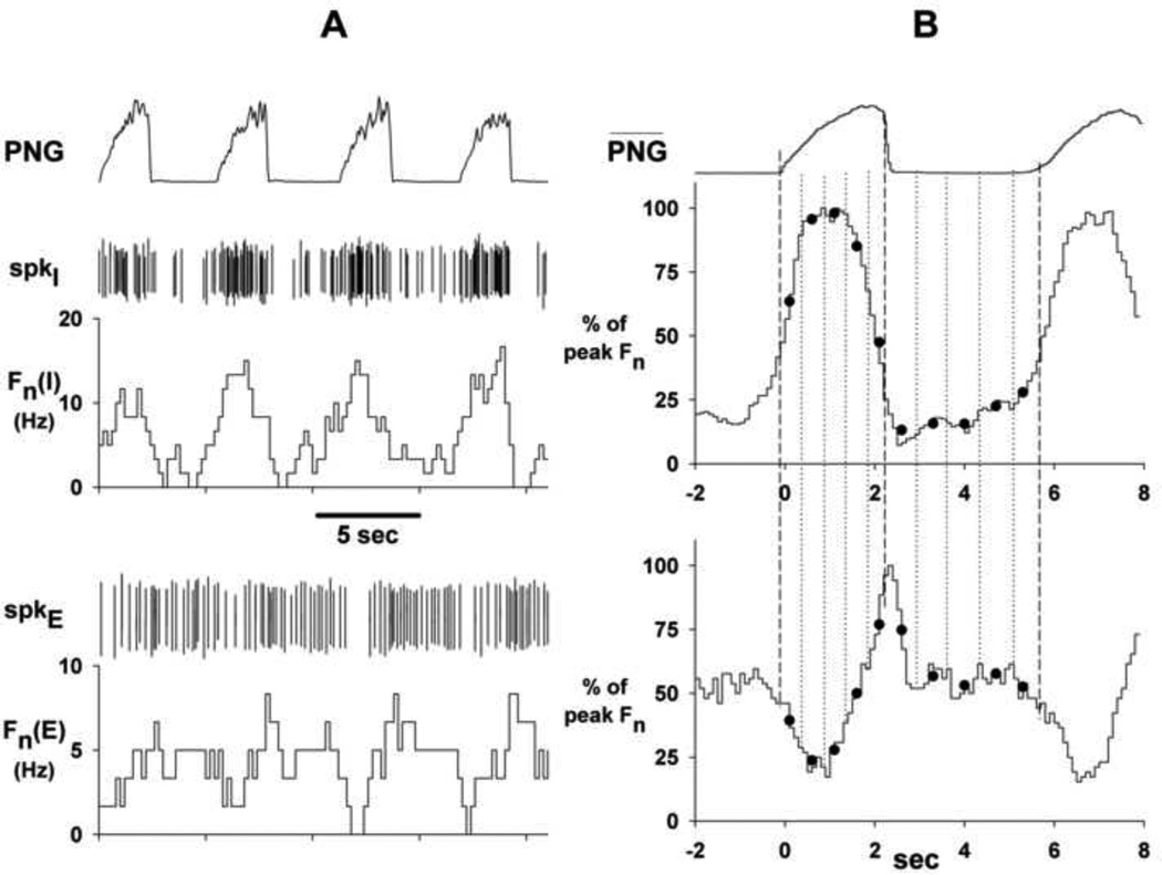
The discharge patterns of 135 PRG neurons obtained from recordings in a decerebrated dog model (n=12 preparations) were used to develop a method to automatically classify discharge patterns according to their contours. The data were recorded from vagotomized dogs ventilated with an air-O2 mixture and maintained in hyperoxic isocapnia (F_IO2>0.6, end-tidal CO₂ range 40—50 mmHg). Extracellular spike activity was recorded from the PB-KF region using a 16-electrode NeuroNexus probe. The electrodes were linearly arranged with an inter-electrode spacing of 100 µm. The spikes were sorted using Cambridge Electronic Design (CED) Spike2, version 7 software. Timing pulses triggered at the upstroke and post-peak downstroke of the phrenic neurogram were used to create cycle-triggered histograms (CTHs) with 50 or 100 ms bins. The CTHs are expressed in terms of percent of peak discharge frequency (Fn), since the emphasis is on the contour of the discharge pattern rather than absolute discharge frequency (amplitude). For each CTH, the I and E phases were each divided into 5 equal zones from which the average discharge frequency (Fn) was computed, yielding 10 data points (see Fig. 1). Using these data points, each CTH can be represented by a 10-dimensional vector: $\overrightarrow{X}=[X_1,X_2,\dots X_{10}]$. These 135 vectors (N=135 neurons) formed the data set that was then subjected to subgroup assignment (clustering) using a modified K-means method (e.g., Aravind et al. 2010). In preliminary analyses, vector lengths of 8, 12, and 16 were also examined to gain insight into the optimal vector length for best discrimination.

Figure 1.

Two examples illustrating data preparation for the clustering procedure. Panel A: spike activity (CED Spike2 wavemark signals) and corresponding rate meter recordings of an I (upper) and E (lower) PRG neuron. Panel B: Corresponding CTHs and time-averaged phrenic neurogram (PNG-bar; 31 cycles). Dots: 5 temporally equidistant values during I-phase and 5 during the E-phase are selected for each vector representation of neuronal pattern. Time zones are indicated by the vertical dashed and dotted lines. See text for more details.

2.1 K-Means Method

For each cluster (subgroup), an initial pattern (10D vector) is required as the starting point of an iterative procedure. A representative or typical example of a commonly occurring pattern from the data set was selected for each cluster. It is important that each selected pattern is visibly different from the other patterns, otherwise two or more clusters will overlap. In this report 7 clusters were designated based on initial patterns such as augmenting and decrementing I and E, IE-EI-phase spanning, and NRM. To determine if an optimal number of clusters was obtained, the data were further examined using a relative distance matrix and a plot (F(k) vs. k) related to the contribution each additional cluster makes to the reduction in overall statistical variance of the data set, adapted from the analysis of Pham et al. (Pham et al. 2004) (see Results 3.3).

The next step is to compare each member (neuronal 10-D vector) of the data set, one at a time, to each of the 7 selected 10D cluster patterns, ${\overrightarrow{C}}_j=[C_{j1},C_{j2},\dots C_{j10}]$ for j = 1–7 and determine which cluster, j, is the closest in terms of vector distance. Specifically, the Euclidean distance (D) is calculated (Eq. 1).

$$D_j=\sqrt{{[(X_1-C_{j1})+(X_2-C_{j2})+\dots (X_{10}-C_{j10})]}^2}$$ Eq (1)

where j = 1 to 7 is the cluster number and X_i and C_i are corresponding vector components of the data-set member vector and the cluster centroid vector (see below for definition of centroid), respectively. The data vector with the shortest distance to a given cluster is assigned to that cluster and the shortest distance is saved and used to calculate the overall iteration error of the complete data set. This procedure is repeated for each member of the data set, in this case N=135. The overall error is the average value of the minimum distances for all N neurons. The next step is to update the C_i values of each cluster. This is done via averaging the data-set member vectors that belong to each cluster (Eq. 2).

$${\overrightarrow{C}}_j=\frac{1}{N_j}\sum _{j=1}^{N_j}\overrightarrow{X_j}$$ Eq (2)

Where N_j is the number of the neuron patterns associated with the j-th cluster. The updated averaged cluster vector is also referred to as the centroid. The above procedure is repeated with the updated centroid vectors and the overall minimum error is noted. Typically less than 10 iterations were required for convergence. Appendix A. gives the details of the implementation of the procedure using the SigmaPlot application software.

2.2 Weighting of 10 D-vector to reduce effects of outliers on centroid

As a refinement to the clustering method, we have found that applying weighting factors to each of the neuron vectors assigned to a given cluster can reduce the overall error. This process assigns less weight to those vectors that are furthest away from the centroid, such that the shape of the centroid is not distorted by an “outlier” vector. A weighting scheme that works well is a decaying exponential of the form:

$$w_j=\text{exp}[-\alpha (D_j-D_{\text{min}})/(D_{\text{max}}-D_{\text{min}})]$$ Eq (3)

where w_j is the weighting factor of the j-th neuron, α is a constant, D_j, D_min, and D_max are the individual, minimum and maximum vector distances from the centroid. For α = 1, when D_j = D_min, w_j = 1 and when D_j = D_max, w_j = ~0.37. The updated centroid has the form:

$$\overrightarrow{C}=\sum _{j=1}^{\mathit{\text{Nj}}}{w}_j{\overrightarrow{X}}_j/\sum _1^{\mathit{\text{Nj}}}{w}_j$$ Eq (4)

3. Results

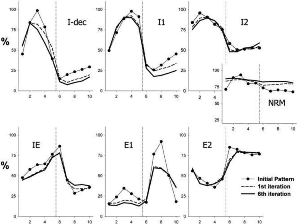
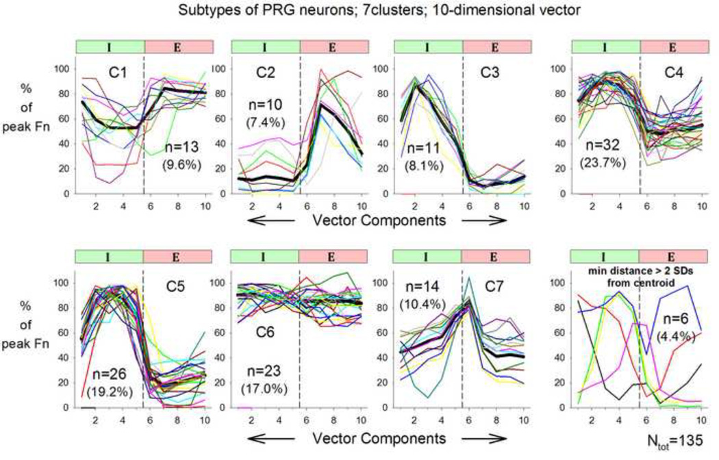
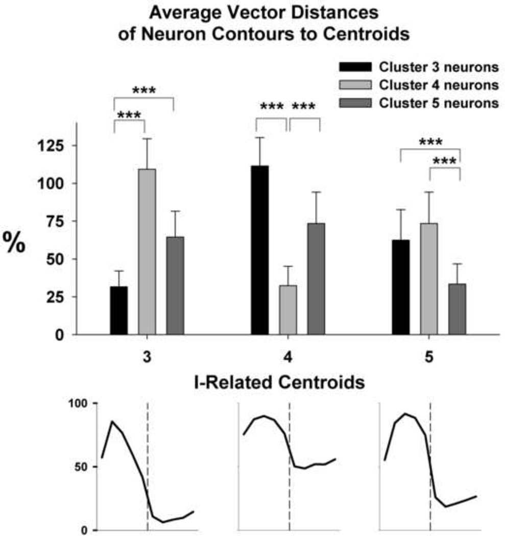
The morphology of a centroid changes noticeably with the first and sometimes second iteration but then stabilizes with only minor additional changes (e.g. Fig. 2). We tested the effects of 9 different sets of 7 initial contours chosen from the data set on the contours of the final 7 centroids after additional iterations failed to reduce the overall error. The final centroids in 2 instances out of 63 (7 clusters × 9 sets of initial patterns) showed patterns that were visibly different from the others. Thus, it is advisable to use 2–3 different sets of starting contours to verify that the final population contours are consistent and independent of the starting set of patterns. Figure 3 shows the final outcome of the clustering procedure for 135 PRG neuron contours. The clustering procedure separated and assigned the 135 individual neuron contours satisfactorily to the 7 clusters for all but 6 neurons. To better assess the degree of separation, in 3 I-related clusters (C3, C4 and C5) the vector distances from the neuron vectors to each of the 3 centroids were calculated and compared (Fig. 4, means and SDs). For each of the 3 centroids, the mean distances from the two non-corresponding data sets were 2 to 5 times greater (p-values < 0.0001) than the distance from its corresponding data set. This confirms that the clustering process was able to adequately separate the neuron contours despite all 3 clusters having I-related centroids.

Figure 2.

Pattern convergence as a function of iteration. Note that after the 1^st iteration the resulting centroid remains close to the final (6^th) iteration.

Figure 3.

Results of the clustering procedure: Traces of individual neuron patterns are superimposed on the centroids (thick lines) that resulted in the smallest overall error. Number of neurons in each cluster and percentage (%)/cluster are indicated for clusters C1-C7. Lower right panel: patterns that did not fit well with any of the 7 clusters.

Figure 4.

Degree of separation in vector distances (D) of neurons assigned to one centroid compared to distances of those neurons to other similar centroids is shown. E.g., the average D of cluster 3 neurons to centroid 3 (black bar, left panel) is significantly different from the average Ds for neurons assigned to clusters 4 and 5 to centroid 3. ***: p<0.001. Vertical dashed lines: I-E transition point.

3.1 Effect of weighting factor

The addition of a weighting factor in updating the centroids of each iteration was evaluated by comparing the clustering results to the result without weighting. α-values (Eq. 3) of 1 and 2 were used, which yields weights of 0.368 and 0.135 to the neuron vector with the greatest distance to the centroid, respectively. The overall error decreased with the increases in α-values, but such decreases were very modest (e.g. 37.18 to 36.77%). The increase or decrease in the number of neurons assigned to a specific cluster (i.e. number of contours reclassified) was only 1 to 2. Visual inspection of the contours that were reassigned from one cluster to another by the addition of weighting indicates an increase in discrimination. However, the weighting factor had no discernible effect on the contours of the final centroids (data not shown).

3.2 Number of vector components

The effect of the number of vector components on pattern discrimination by K-means clustering was evaluated by increasing the number of dimensions from 8 to 10 to 12 to 16 (data not shown). The I- and E-phases of the CTHs were divided into 4^ths, 5^ths and 6^ths for dimensions 8, 10 and 12. For 16 components, the I-phase was divided into 6^ths and the E-phase in 10^th s because the E-phase is typically longer. While the increase in dimensions increase resolution of the pattern itself, it did not significantly improve discrimination of the patterns by the clustering process. In fact, iterations of the 16-component vector became unstable and would not converge. With increases in dimension, the overall error increases since the Euclidean distance (Eq. 1) increases due to an increase in the number of terms. Visual inspection of the clustering suggests that the increase from 10 to 12 dimensions showed more scatter about the centroids. There were only small differences in the clusters by increasing from 8 to 10 dimensions. However, since there are some neuron patterns with narrow peaks, we decided to use a 10 dimensional vector for added pattern resolution. There appears to be an optimal point between the degree of pattern resolution and stable clustering, where the neuron patterns conform tightly to the centroids.

3.3 Methods to assess the optimal number of clusters

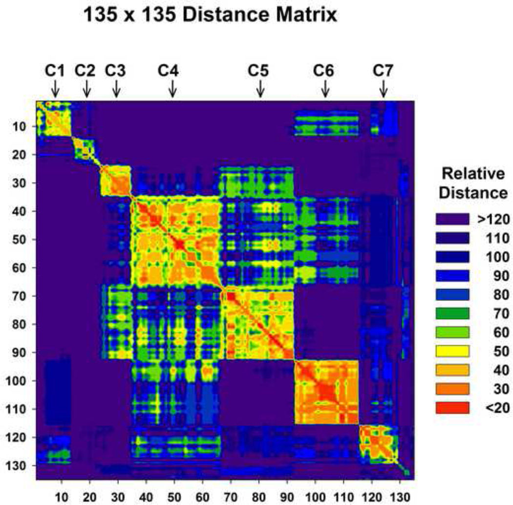
One of the limitations of the K-means clustering is that the number of clusters, k, must be specified before the algorithm can be applied. Finding the appropriate number of clusters for a given dataset is generally a heuristic, trial-and-error process. To better assess if the selected number of clusters was appropriate, we also used a matrix of the relative distances. Each cell in this square matrix contains the Euclidian distance between one member of the data set with another member of the data set. In this case there are 135 × 135 or 18225 cells. The members were ordered along the x and y axes according to the clustering results shown in figure 3. The Distance Matrix shows 7 discrete blocks corresponding to the 7 clusters indicated (Fig. 5, top) along the diagonal and suggests that k=7 represents an optimal number of clusters. The number of members associated with each of the clusters dictates the sizes of the blocks. The orange spots adjacent to the C4 and C5 suggest that those members could belong to either C4 or C5. For the other 5 clusters, the contrast with members outside the cluster is remarkable.

Figure 5.

The Distance Matrix shows the 7 clusters as 7 discrete blocks along the diagonal and suggests that k=7 represents an optimal number of clusters . The sizes of the blocks are dictated by the number of members associated with each of the clusters. The orange spots adjacent to the C4 and C5 suggest that those members could belong to either C4 or C5.

Another method to determine the optimal value of k was developed by Pham et al. (2004). It uses a measure of the distortion of a cluster is a function the distance between cluster members and the cluster centre calculated as:

$$I_j=\sum _i^{\mathit{\text{Nj}}}{(X_{\mathit{\text{ji}}}-C_j)}^2$$ Eq (5)

where I_j is the distortion of cluster j, C_j is the center of the cluster j, N_j is the number of members belonging to cluster j. Each cluster is represented by its distortion and its impact on the entire data set is assessed by its contribution to the sum of all k distortions, S_k:

$$S_k=\sum _{j=1}^K{I}_j$$ Eq (6)

The quantity S_k, in terms of ANOVA, represents the total sum of squares without the correction term. Pham et al. (2004) developed a function:

$$F(k)=S_k/{\alpha }_k{S}_{k-1}$$ Eq (7)

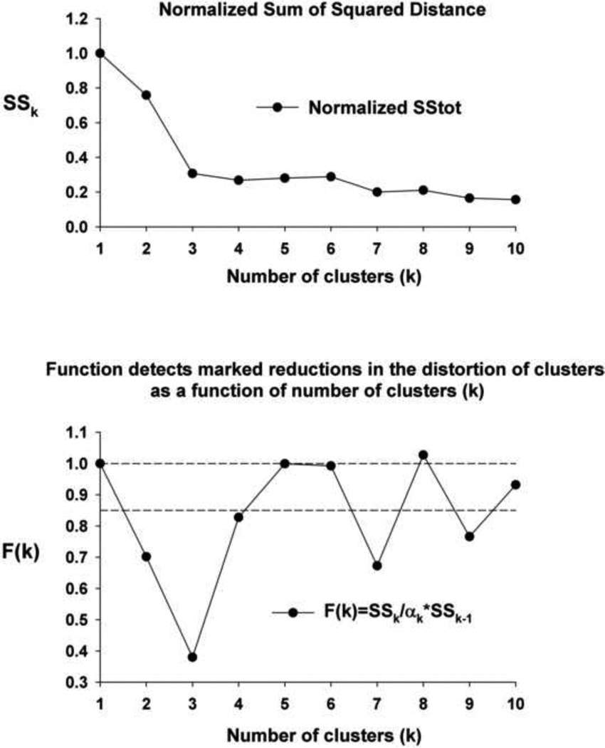
where F(k)=1 for k=1, otherwise F(k) is according to Eq(7). α₁=1, α₂=1–3/4N_d, where N_d =10 is dimension of the vector and α_k= α_k-1 + (1- α_k-1)/6. The range of α_k in our case was from 1 to 0.925. Essentially, F(k) is ~ratio of S_k to S_k-1. We have found that the sum of squares total (SS_total) from an ANOVA table, which includes the correction term, provides a more sensitive F(k). The plot of SSk vs k (Fig. 6 upper) shows a rapid decrease for k from 1 to 3 and then a more gradual decrease for k>3. However the plot of F(k) vs k (Fig. 6 lower) shows several points below a threshold value of 0.85, which the study of Pham et al.(2004) concluded that any k with a corresponding F(k)<0.85 could be recommended for clustering. F(k) is less than 0.85 for k=2,3,7 and 9. For k=2, I- and E-neurons formed separate clusters. For k=3, I-, E- and NRM-neurons formed separate clusters. For k=7 (F(7)=0.67), the centroids are shown in figure 3, and for k=9 (F(9)=0.77), the PRG I-neurons of C4 and C5 (Fig. 3) were subdivided into 3 clusters, with the 3^rd cluster intermediate to C4 and C5.. The incremental improvement in SS_k by adding the 7^th cluster is clearly greater than that for adding the 9^th cluster.

Figure 6.

Statistical Method to determine the optimal number of clusters of the data set. Upper panel: Plot of the normalized sum of squared distance (SS_k) vs. the number of clusters (k) decreases as a function of k. Lower Panel: Plot of a function of the ratio of SS_k to SS_k-1 enhances the detection of the relative decrease in total variance of the data set that the addition of cluster k contributes. See text for details.

3.4 Main subtypes of canine PRG neurons based on discharge pattern

The clustering results of the canine PRG neuronal patterns (Fig. 4) indicate that 69 of 135 (~51%) neurons show inspiratory-related patterns (clusters C3, C4 & C5, Fig. 4). The centroid of cluster C3 shows a delayed I-decrementing pattern, while the centroids of clusters C4 and C5 show I-parabolic patterns, where peak discharge occurs before the end of the I-phase, with differing levels of activity during the E-phase. The centroids of clusters C1 and C2 show distinct E-phase related activity with differing levels of I-phase activity, but represent only 16% of the PRG neurons. The centroid of cluster C7 increases in a ramp-like pattern during the I-phase and reaches a peak slightly after the I-E phase transition, then decays rapidly during the early E-phase. This type of contour, consisting of ~11% of the canine PRG neurons, has been referred to as an I-E phase spanning pattern (Segers et al. 2008). NRM neurons made up 17% of the population of 135 neurons. Also shown in figure 4, lower right, are 6 neuron patterns that did not fit well with any of the 7 cluster centroids, that is, their distance was greater than 2 SDs from the mean distance of the clustered neurons.

3.5 Amplitude of modulation calculation

The amplitude of respiratory-related modulation of the PRG neuron patterns was calculated as:

$$\%M=100\times \left(\right(F_{\text{max}}-F_{\text{min}})/F_{\text{max}})$$ Eq (5)

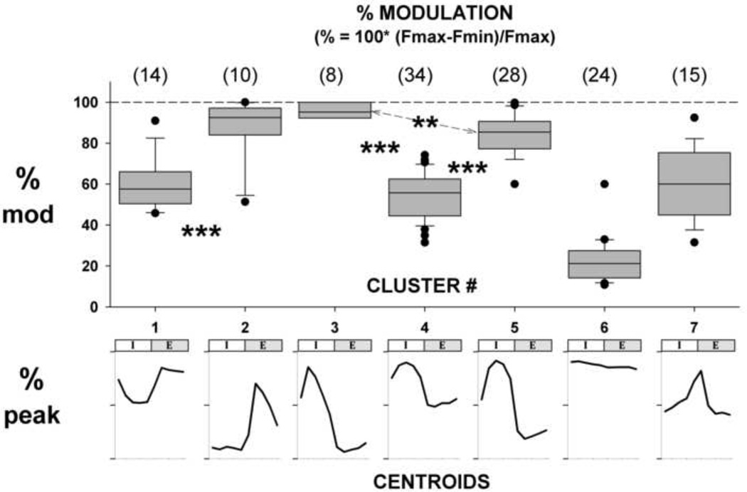
where, F_max and F_min are values taken from 10-component vector representation of the CTH. Within each of the clusters, %M was calculated for each neuron and the results are shown as a box plot in Fig. 7. As a visual aid, each of the corresponding centroids is shown below the modulation data. Visual inspection shows that there is a good correlation between the centroid pattern and the degree of modulation. As expected, cluster #3 (I-dec) shows the highest degree of modulation, whereas cluster #6 (NRM) shows the lowest degree of modulation with the other patterns showing intermediate degrees of modulation. There are significant differences between the two types of E-neurons and the three types of I-neurons as indicated by asterisks. The median values for each cluster are listed in the figure legend.

Figure 7.

Box plots of % Modulation for each cluster show 25, 50, & 75 percentiles (gray fill, bottom, mid, & top) and 10 & 90 percentiles. Circles: data <10 and >90. Median values: (1) 57.6%, (2) 92.5%, (3) 95.2%, (4) 55.7%, (5) 85.4%, (6) 21.2%, (7) 60.0%. **: p<0.01; ***: p<0.001. See text for details.

4. Discussion

The K-means clustering method offers a robust objective means of both automatically categorizing neuron patterns and establishing the underlying archetypical contours of neuron subtypes based on the discharge patterns of a group of neurons. Changing the number of clusters and inspecting the resulting plots similar to those shown in figure 3 can determine the optimal number of clusters. If for example only 3 clusters are used, then the neuron patterns fall into I-, E- and NRM categories. However, since in our experimental neuronal data set there was more than one subtype of I and E neuron pattern, as well as phase-spanning types, we chose to analyze 7 clusters. Two additional methods were used to confirm that the number of clusters, 7 was optimal for our data set. The relative distance matrix of figure 5 shows 7 rather distinct blocks corresponding to the 7 clusters. A second method, adapted from the study of Pham et al. (2004), shows how each additional cluster incrementally contributes to lowering the overall variance of the data set (Fig. 6). By plotting the ratio of the sum of squares, SSk/SSk-1, we increased the sensitivity of the method (Fig. 6, lower). In our case, with a k=7 the F(k)(0.67) is markedly below the threshold (F(k)=0.85) suggested by the analysis of Pham et al. (2004). With K=9, F(k)(0.77) is also below the threshold and the corresponding centroids mainly show that clusters C4 and C5 (Figs. 3 & 4) are further subdivided into 3 clusters, each similar in shape but with a different level of E-phase activity. Thus, this method does provide guidance on choosing the value of k, but the matter of discretion and the level of detail are still up to the investigator. For the purpose of discussion, a k-value of 7 will be used.

In our sample of 135 neurons, the method resulted in 3 I-related types and only one phase spanning (IE) type, but neurons in cluster #4 (Fig. 3) may be considered EI phase-spanning, since activity is increasing as the E-phase progresses. Choosing a greater number of clusters will result in centroids with only subtle differences in contours, and the results will depend on the initial starting patterns assigned to each cluster. Choosing distinct patterns will improve the separation. To verify that the final centroids, after a sufficient number of iterations, are representative the process should be repeated with a different set of initial patterns. In this study we used 9 different sets of patterns and only 2 of 63 (9×7) contours showed significant differences. A method to estimate how distinct one cluster is from another with a similar pattern is shown in figure 4. The method calculates the distance statistics of vectors assigned to one of the clusters to the centroid belonging to the other cluster and compares those statistics with the vectors assigned to their corresponding centroid. The results of this method, shown in figure 4, indicate that related but distinct clusters had distances that were 2–5 fold larger that those corresponding to the assigned cluster.

The use of weighting factors for updating the centroid, after each iteration, resulted in small decreases in the overall error (average distance of neuron vectors from their assign clusters) by giving less weight to the vectors furthest from their currently assigned centroid. It also allowed more reliable assignment of contour patterns that were difficult to classify before weighting. It is possible to use other functions to calculate the weighting factors such as a line with a negative slope and a y-intercept of 1.0 at D_min.

Based on a large enough, representative sample of neuron patterns, the final centroids, which represent each neuron subtype contour, can be used to categorize subsequent neurons to one of the centroids, by calculating the vector (Euclidean) distances to each centroid and assigning the neuron pattern to the one with the shortest distance. The method may also be useful for exploring within the data set the number of neurons with a particular contour, by using that contour as one of the initial centroids before the iteration process begins.

4.1 Other methods

In a detailed quantitative analysis, Carroll et al. (2013) used multiunit extracellular recording in the in vitro pre-Bötzinger complex to identify and characterize the rhythmic activity of 951 cells. Cycle-triggered rate functions, triggered from the onset of the population burst, for each cell were normalized, demeaned and digitized and represented by a vector of 301 values (250 samples/sec × 1.204 sec). The data set as a whole was then analyzed with principal component analysis (PCA), nonlinear dimensionality reduction, and hierarchical clustering techniques. However, none of these techniques revealed categorically distinct functional cell classes, but a continuous distribution of firing rate behavior, especially within the I-phase related population. Visual inspection of the patterns shown in their figures 3 and 5 shows that the smooth shapes are very similar and not very distinctive. It may be possible that the application of the PCA method to respiratory-related discharge patterns from in vivo preparations, which tend to show more distinctive patterns, will provide a quantitative means of classifying those rhythmic neurons. This possibility was discussed in some detail at a presentation at The 12th Oxford meeting in Almelo, Netherlands, 2012 by Kendall Morris et al. (personal communication). However, data dimensionality reduction where only the first 2–3 components are used (PCA method) will most likely not be able to discriminate contours with distinct but subtle differences. In addition, usually some method of clustering similar to K-means is used following PCA to classify the results and thus requires guidance on choosing the number of clusters. The method we present here, using K-means clustering of 10-dimensional vectors is relatively straight forward, intuitive in nature and very computationally efficient.

4.2 Subtypes of PRG neurons

The clustering results based on 135 canine PRG neurons recorded from the medial and lateral parabrachial regions separated into the 7 patterns shown by the centroids in figure 7 lower. These data were recorded from vagotomized, ventilated, decerebrate dogs during isocapnic hyperoxia (range: 40–50 mmHg; F_IO2>0.6). What emerged were 3 types of I-phase-related neurons (70/135, ~52%), 2 types of E-phase related neurons (24/135, ~18%), 1 type of IE phase-spanning neurons (15/135, ~11%) and NRM neurons (24/135, ~18%). The I-decrementing neurons were the fewest (8/135, ~6%) but had the highest degree of modulation (median: ~95%).

In a vagotomized, decerebrate cat model during normcapnia (4–4.5%), Segers et al. (2008) categorized 145 PRG neurons into 4 basic subtypes based on the time of peak discharge within the respiratory cycle and a NRM subtype: I (19%), IE (14%), E (8%), EI (6%) and NRM (53%). Many of the contours shown in figure 2B of Segers et al. (2008) are similar to those in the dog. Many of the EI neurons would fit into one of the canine E subtypes and there was no feline I-decrementing category. In addition, their PRG population consisted of more NRM neurons than our canine set (53% vs. 18%).

In urethane anesthetized, vagotomized, ventilated, isocapnic (range: 5.0–5.5%; F_IO2=0.4) adult rats, Song el al. (2006) studied the morphology and discharge patterns of 14 PRG neurons and found patterns corresponding to I (14%), IE (14%), early-E (21%), late-E (14%), and EI (36%). The CTHs show that most of these neurons were highly respiratory modulated (silent periods within the cycle) and only 4/14 show tonic background activity (Fig. 2 in Song et al. (2006)). Their EI neurons show considerable activity during the I-phase. In sodium pentobarbitone anesthetized, vagal nerve intact, ventilated, isocapnic (range: 4–5%) adult rats, Ezure and Tanaka (2006) classified PRG neurons (n=235) into 6 types: I-neurons (21%), EI phase-spanning neurons (40%), IE phase-spanning neurons (7%), E-decrementing neurons (9%), augmenting E (E-AUG) neurons (12%), and whole-phase E-neurons (11%). The examples in their figures 1 and 2 show silent periods, which suggest a very high degree of respiratory related modulation. Since they used strip chart recordings and did not generate CTHs, it is not possible to use the clustering technique to automatically classify their PRG neurons.

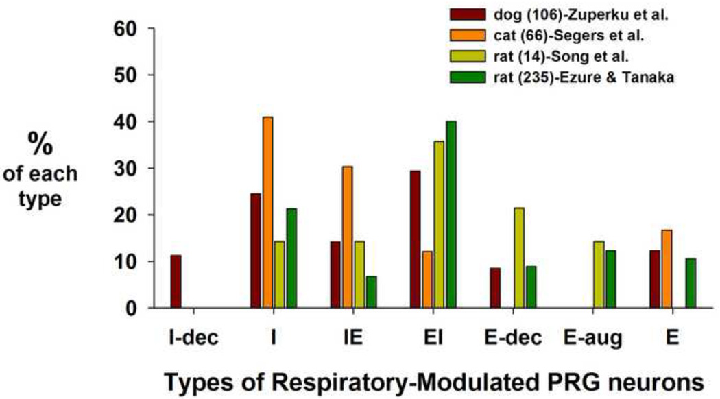
A comparison of the classifications of the respiratory-modulated PRG neuron types for the different species described above is shown in figure 7 (percentages recalculated without accounting for NRM neurons). It appears that there is a greater percentage of the I and IE types in the cat compared to the dog and rat. On the other hand, the cat shows a smaller percentage of EI type neurons. It also appears that E-neuron types represent a smaller portion of the overall PRG population.

4.3 Amplitude of respiratory modulation

Regarding quantification of the amplitude of respiratory modulation of pontine neurons, the eta-squared statistic (η²), introduced by Orem and Dick (1983) has been used in several studies (e.g. Dick et al. (2008); Segers et al. (2008)). The effect size or η² = SS_between/SS_total, where SS is the sum of squares can be calculated from an analysis of variance (ANOVA) table. However, data from individual respiratory cycles must be used. In this study as well as others where CTHs are generated, it is not possible to calculate η² values, since CTHs represent mean frequencies only. To estimate the amount of respiratory-related modulation we used data derived from CTHs, that is, the average discharge frequency for the 10 time zones as shown in figure 1. These values represent a smoothed CTH that minimized the effects of large transient peaks or troughs in the calculation of the modulation index (Eq. 5). Figure 7 shows that this index reflects the excursion of the centroids for each of the clusters. In addition, η² values are sensitive to the duty-cycle of the pattern independent of magnitude of the phasic component of a pattern. For example, for a short duration discharge pattern the η² value would be much lower than that for the same pattern that filled most of the I- or E-phase (~ 50% duty cycle).

4.4 Summary and conclusions

The discharge patterns of 135 canine PRG neurons were classified using an automated K-means clustering method. Using 7 clusters, 6 distinct phasic patterns were recognized and one NRM pattern. The cluster centroids can be used as templates to classify the discharge patterns of sets of canine PRG neurons from other studies. However, the templates may be species specific and should be based on data from the species of interest. The method offers an unbiased approach to assigning neurons to a subtype category. This study also shows the various subtypes of PRG neurons that are present in canine species. The percentages of each of the canine PRG neuron subtypes were compared with those for cats and rats and show some similarities (Fig. 7). However, the criteria used to assign patterns to specific categories appear to be different in each study and may have influenced the subtype distribution statistics. This study suggests that the method described is straight forward, simple to use, and works well to discriminate and classify phasic neuronal discharge patterns.

Figure 8.

Comparison of the distribution of subtypes of PRG neurons among species.

Highlights.

• Clustering method automatically classifies neurons according to discharge Pattern

• This method also derives an average subgroup contour of each class

• This method was implemented via SigmaPlot User-Defined transform code

• 135 canine PRG neurons were classified into 7 distinct subtypes

• The method offers a robust objective means of categorizing neurons into subtypes

APPENDIX A. SigmaPlot Transform code for K-means clustering

Figure A1 shows the steps used to implement clustering procedure. The details and code used for clustering neuronal discharge patterns are given below. The method was implemented using SigmaPlot’s data worksheet, graphics, and transform language. It uses worksheet column math and logic functions to increase computational efficiency. In this case of classifying 135 neuronal patterns, execution time was less than 2 seconds per iteration. At the beginning of each iteration, the program transfers the updated centroid values of the 7 clusters from the previous iteration in columns 30–36 into columns 20–26. Unlike other programming languages, SigmaPlot transform code requires using designated cells as variables that are incremented within loops.

Figure A1.

Steps used to implement clustering.

Column Assignments used in SigmaPlot Program
Columns 1–4, Rows 1-N (# of neurons in data set) Each neuron’s # corresponds to the row# it is located in	Neuron information: date, neuron channel#, location & etc.
Columns 5,18, & 28	Low # rows used for intermediate calculations
Columns 6–13, rows 1–49	Contains sorted neuron#s assigned to each of the 7 clusters and col#13 is for neurons that don’t fit well with any of the clusters
Columns 6–13, rows 50–55	Cluster summary results for each of the 7 clusters: mean (vector distance of neurons in the cluster), SD, minimum, maximum, mean+2SDs, and number of neurons in cluster.
Columns 16 and 17 (N rows)	Minimum vector distance of neuron vector to one of the centroids determines the cluster# it is assigned to (col. 17)
Col 18, Row 1	Overall average minimum error of each iteration
Columns 20–26, 10 rows	Initial cluster vectors (n=7), or after 1st iteration, 7 vector centroids used for distance calculations
Column 27, rows 1–10	Plotting index 1–10
Column 29, rows 1–7	Number of neurons in each cluster
Columns 30–36, rows 1–10	Updated centroids following iteration
Columns 37 & 38	Intermediate calculations for determining weighting factors
Columns 40-(40+135=175), rows 1–10 N=135 neurons in this study	Neuron contour vectors.
Columns 180 −330	After final iteration, for each cluster, assigned neuron vectors are placed in adjacent columns to facilitate plotting. An empty column separates each cluster data.

SigmaPlot transform code for the K-means routine with weighted mean

sw1=1     ; sw1=1 enables transfer of cluster results to the print area

          ; sw1=0 skips the above step

a=2       ; exponential rate factor, a=0 (no weighting)

cell(18,3)=a

n=count(col(4))  ; number of neuron vectors

nclust=7         ; number of clusters



for c1=0 to nclust-1 do   ; transfer centroid updates to cluster block

col(20+c1)=col(30+c1)

end for



for i=1 to n do     ; loop for n vectors

cell(5,1)=10000

for k=1 to nclust do     ; number of clusters

dd=total((col(39+i)-col(19+k))^2)

vmag=sqrt(dd)       ; Euclidian distance from points to centroids

; cell(19,k)=vmag

if (vmag<=cell(5,1)) then

cell(5,1)=vmag

kmin=k

cell(16,i)=vmag     ; min distance of vector “i” to one of the centroids

cell(17,i)=kmin     ; corresponding cluster/centroid #

end if

end for

end for



cell(18,1)=total(col(16))/n     ; average error distance for current iteration



for ck = 1 to nclust do      ; initialize centroid update columns

for i1=1 to 10 do            ; starting at col (30)

cell(29+ck,i1)=0

end for

col(5+ck)=if(col(5+ck)>=0,"","")   ; clear col containing neuron #s within a specific cluster

end for

col(13)="”                  ; clear col(13)



for j1=180 to 330 do        ; clear cells for new plots

for j2=1 to 10 do           ; 10 components of CTH vector

cell(j1,j2)=""

end for

end for



for k2= 1 to nclust do     ; Create a list of vector #s for each cluster

cell(28,3)=0                 ; initialize summing variable for # of vectors in each cluster

for i2=1 to n do

if (cell(17,i2)=k2) then

cell(28,3)=cell(28,3)+1      ; increment index

cell(5+k2,cell(28,3))=i2     ; col # of cluster sorted neuron

end if

end for                  ; end i2 loop

cell(29,k2)=cell(28,3)

end for                  ; end k2 loop



for k3=1 to nclust do  ; This section calculates statistics for vector distances within cluster “k3”

    ; weighting factors and updates centroid

col(38)=if(col(38)>=0,"","")  ; delete old data in cols 37 & 38

col(37)=if(col(37)>=0,"","")

col(38)=col(16)[col(5+k3)]     ; put min. distance values for cluster k3 into col(38)

d=col(38)

col(332+k3)=if(col(332+k3)>=0,"","")    ; delete data in cols 333---

col(332+k3)=d                           ; put min distances in cols 333+

dmin=min(d)             ; find min, max, mean, SD, & mean+2SDs

dmax=max(d)

ddiff=dmax-dmin

cell(5+k3,50)=mean(d)

cell(5+k3,51)=stddev(d)

cell(5+k3,52)=dmin

cell(5+k3,53)=dmax

sdx2=cell(5+k3,50)+2*cell(5+k3,51)

cell(5+k3,54)=sdx2

cell(5+k3,55)=count(d)             ; find # of neurons/cluster

col(37)=exp(−a*(d-dmin)/ddiff)     ; calculate weighting factor for each neuron



n3=cell(29,k3)     ; number of neurons per cluster

for i3=1 to n3 do

col(29+k3)= col(29+k3)+cell(37,i3)*col(39+cell(5+k3,i3))     ; summing weighted vectors

end for                                                      ; for updated centroid



wtot=total(col(37))     ; sum of weighting factors

col(29+k3)=col(29+k3)/wtot     ; updated centroid

end for     ; k3



if sw1=1 then

cell(28,5)=180          ; group clustered data for plotting

cell(28,7)=0        ; initialize summing variable for the row # of an outlier

for k4=1 to nclust do

for i4=1 to cell(29,k4) do             ; # of neurons in cluster k4

cnk=cell(28,5)

nn1=cell(5+k4,i4)                      ; neuron # within cluster k4

if cell(16,nn1)>cell(5+k4,54) then     ; dmin>2×SD

 cell(28,7)=cell(28,7)+1              ; increment row index

 jdex=cell(28,7)

 cell(5+k4,i4)=136                 ; replace nn1 with 136 (shifted is col (175) =null vector )

 cell(13,jdex)=nn1                 ; cell for outliers in category 8 i.e., d>2SD

end if

nn2=cell(5+k4,i4)

col(cnk+i4)=col(39+nn2)

end for   ; i4 loop

cell(28,5)=cell(28,5)+cell(29,k4)+1  ; update col # for next cluster set

end for   ; k4 loop

for i5=1 to jdex do

col(cell(28,5)+i5)=col(39+cell(13,i5))  ; loop to place outliers in far right for plotting

end for

end if

REFERENCES

- Alheid GF, Milsom WK, McCrimmon DR. Pontine influences on breathing: an overview. Respir Physiol Neurobiol. 2004;143:105–114. doi: 10.1016/j.resp.2004.06.016. [DOI] [PubMed] [Google Scholar]
- Aravind H, Rajgopal C, Soman K. A Simple Approach to Clustering in Excel. International Journal of Computer Applications(0975--8887) 2010;11:19–25. [Google Scholar]
- Carroll MS, Viemari JC, Ramirez JM. Patterns of inspiratory phase-dependent activity in the in vitro respiratory network. J Neurophysiol. 2013;109:285–295. doi: 10.1152/jn.00619.2012. [DOI] [PMC free article] [PubMed] [Google Scholar]
- Cohen MI. Switching of the respiratory phases and evoked phrenic responses produced by rostral pontine electrical stimulation. J Physiol (London) 1971;217:133–158. doi: 10.1113/jphysiol.1971.sp009563. [DOI] [PMC free article] [PubMed] [Google Scholar]
- Dick TE, Shannon R, Lindsey BG, Nuding SC, Segers LS, Baekey DM, Morris KF. Pontine respiratory-modulated activity before and after vagotomy in decerebrate cats. J Physiol. 2008;586:4265–4282. doi: 10.1113/jphysiol.2008.152108. [DOI] [PMC free article] [PubMed] [Google Scholar]
- Dutschmann M, Dick TE. Pontine mechanisms of respiratory control. Compr Physiol. 2012;2:2443–2469. doi: 10.1002/cphy.c100015. [DOI] [PMC free article] [PubMed] [Google Scholar]
- Ezure K, Tanaka I. Distribution and medullary projection of respiratory neurons in the dorsolateral pons of the rat. Neuroscience. 2006;141:1011–1023. doi: 10.1016/j.neuroscience.2006.04.020. [DOI] [PubMed] [Google Scholar]
- Orem J, Dick T. Consistency and signal strength of respiratory neuronal activity. J Neurophysiol. 1983;50(5):1098–1107. doi: 10.1152/jn.1983.50.5.1098. [DOI] [PubMed] [Google Scholar]
- Pham D, Dimov S, Nguyen C. Selection of K in K-means clustering. Proceedings of the Institution of Mechanical Engineers, Part C: Journal of Mechanical Engineering Science. 2004;219:103–119. [Google Scholar]
- Prkic I, Mustapic S, Radocaj T, Stucke AG, Stuth EA, Hopp FA, Dean C, Zuperku EJ. Pontine mu-opioid receptors mediate bradypnea caused by intravenous remifentanil infusions at clinically relevant concentrations in dogs. J Neurophysiol. 2012;108:2430–2441. doi: 10.1152/jn.00185.2012. [DOI] [PMC free article] [PubMed] [Google Scholar]
- Segers LS, Nuding SC, Dick TE, Shannon R, Baekey DM, Solomon IC, Morris KF, Lindsey BG. Functional connectivity in the pontomedullary respiratory network. J Neurophysiol. 2008;100:1749–1769. doi: 10.1152/jn.90414.2008. [DOI] [PMC free article] [PubMed] [Google Scholar]
- Song G, Yu Y, Poon CS. Cytoarchitecture of pneumotaxic integration of respiratory and nonrespiratory information in the rat. J Neurosci. 2006;26:300–310. doi: 10.1523/JNEUROSCI.3029-05.2006. [DOI] [PMC free article] [PubMed] [Google Scholar]
- St-John WM. Neurogenesis of patterns of automatic ventilatory activity. Progress in Neurobiology. 1998;56:97–117. doi: 10.1016/s0301-0082(98)00031-8. [DOI] [PubMed] [Google Scholar]