Prediction of microRNA target genes using an efficient genetic algorithm-based decision tree

Highlights

• •We used a genetic algorithm (GA) in combination with C4.5 decision tree for prediction of miRNA targets.
• •The GA-based decision tree was used for selection of the best rules out of the rule sets.
• •We used a good measure (weighted F-measure) as fitness function.
• •Our method extracted 7 rules, which can be implemented for other similar dataset to prediction of miRNAs target.
• •We achieved 93.9% and 97.1% accuracy of classification for two previously published datasets.

Abstract

MicroRNAs (miRNAs) are small, non-coding RNA molecules that regulate gene expression in almost all plants and animals. They play an important role in key processes, such as proliferation, apoptosis, and pathogen–host interactions. Nevertheless, the mechanisms by which miRNAs act are not fully understood. The first step toward unraveling the function of a particular miRNA is the identification of its direct targets. This step has shown to be quite challenging in animals primarily because of incomplete complementarities between miRNA and target mRNAs. In recent years, the use of machine-learning techniques has greatly increased the prediction of miRNA targets, avoiding the need for costly and time-consuming experiments to achieve miRNA targets experimentally. Among the most important machine-learning algorithms are decision trees, which classify data based on extracted rules. In the present work, we used a genetic algorithm in combination with C4.5 decision tree for prediction of miRNA targets. We applied our proposed method to a validated human datasets. We nearly achieved 93.9% accuracy of classification, which could be related to the selection of best rules.

1. Introduction

MicroRNAs (miRNAs) are known as single-stranded non-coding RNAs ranging in length from 19 to 25 nucleotides (nt). MicroRNAs regulate gene expression in almost all plants and animals. Interestingly, a large number of miRNAs are evolutionarily conserved across species boundaries [1]. In general, miRNA are uncapped, unpolyadenylated small RNAs, which are transcribed by RNA polymerase II into long primary transcripts (pri-miRNAs) [2], [3]. The primary transcripts are processed to mature miRNA in sequential steps by the RNase III endonucleases Drosha in the nucleus [4] and Dicer in the cytoplasm [5]. The mature miRNA is incorporated into an RNA molecule, which induces a silencing complex (RISC) and guides RISC to complementary mRNA targets. Subsequently, the RISC inhibits translation, elongation or triggers the degradation of target mRNA [6].

Overall, miRNAs typically repress gene expression [7]. To date, more than 1500 miRNA genes have been identified in the human genome. Although a large number of miRNAs have been discovered, only a few targets have been identified. Computational predictions of miRNA targets suggest that up to 30% of human protein coding genes may be regulated by miRNAs [8], [9]. This makes miRNAs one of the most abundant classes of regulatory genes in humans. Numerous reports have demonstrated the importance of miRNA-mediated regulation in key processes, such as proliferation, apoptosis, differentiation and development, cellular identity and pathogen–host interactions [10], [11]. However, the mechanisms by which miRNAs act are still not resolved. The first step toward clarifying the function of a particular miRNA is the identification of its direct targets. This is a quite challenging step in animals primarily due to the incomplete complementarities between miRNA and target mRNAs.

Several computational programs exist to predict miRNA targets in animals and plants including PicTar, TargetScan and MiRanda. These programs are based on evolutionary conservation. Despite of many predictions, a limited number of them have been biologically validated. The miRNA targets of plant can be identified straightforward on a genome-wide scale by search for the targets with a high degree of sequence complementarities. Nevertheless, this task cannot be addressed the targets of animal miRNAs. The animal miRNAs pair imperfectly with their targets and act to control translation. The absence of targets with perfect or near-perfect sequence complementarities is prevailed in animal miRNAs. Target prediction in the animal transcriptomes, therefore, needs more complex algorithms because of the imperfect complementarities of miRNA:mRNA pairs [12], [13], [14], [15].

The prediction of miRNA targets in PicTar [15], [16] used in Drosophila and other species is based on the complementarities between miRNA and 3′UTR of mRNA sequence. The false positive rate of this computational tool is estimated to be 30%. TargetScan [12] is another tool for prediction of miRNAs by binding to 3′UTRs of vertebrate transcriptomes. TargetScan is able to predict more than 451 human microRNA targets. TargetScanS [8], a modified version of TargetScan, omits multiple sites in each target and further filters the targets and featured thermodynamic stability. Using this modified procedure, more than 5300 human genes could be predicted as the possible targets of miRNAs. The false positive of this computing tool rates from 22% to 31%. Several researchers endeavored to improve TargetScan efficiency by modification of its algorithm and development of new features [17], [18]. For example, Friedman et al. [17] developed a version of TargetScan that incorporates new genomes and more completely controls for background conservation. MiRanda acts based on the evolutionary relationships between miRNAs and their targets [13], [19], [20]. This tool focuses on the sequence matching of miRNA:mRNA pairs, by estimating the energy of physical interaction. MiRanda was initially developed for predicting miRNA targets in Drosophila [19] and was later extended to find miRNA targets in mammals (human, mouse and rat) and zebrafish [13]. The miRanda algorithm works by scanning for miRNA complementary pairs in the 3′UTR of a mRNA. Using this software, a large number of targets were identified including protein-coding genes in Homo sapiens with the false positive rate of about 24%.

In addition to above mentioned approaches, there are many machine learning algorithms for miRNAs target prediction. Support Vector Machine (SVM) [21], [22], [23], [24], [25], Naïve Bayes [26], [27], Artificial Neural Network (ANN) [28], Pattern Recognition Neural Network (PRNN) [29], ensemble algorithm [16] and other machine learning algorithms [30] have been used for prediction of miRNAs targets.

In the present study, we introduce an efficient genetic algorithm-based decision tree to select the best rules among all extracted rule sets which leads to improve the accuracy of prediction. The proposed method was also compared with several machine learning algorithms.

2. Materials and methods

2.1. Dataset description

We used the dataset of Yan et al. [16] obtained from TarBase database (version 3.0) [31]. TarBase stores a manually curated collection of experimentally verified miRNA targets. The human data were used for training and evaluating of the classifier. The data used by Yan et al. [16] met the following two criteria:

• (1)The binding picture of miRNA-target duplex should be known.
• (2)The target site sequence should match its corresponding reference mRNA sequence provided by NCBI Gene database. Even one single mismatch is not permitted.

Thus, a total of 48 positive and 16 negative examples were collected [16]. Details of the dataset are shown in Table 1. We designated positive samples by 0 and negative samples by 1. This dataset was downloaded from http://www.sciencedirect.com/science/article/pii/S0014579307002761#MMCvFirst, which was presented as supplementary content of Yan et al. [16]. This dataset contains 64 samples and 50 features about miRNAs. Each sample includes distinct features, leading each sample to a special class of target. The features are divided in 4 categories as follow:

• 1.Features calculated over entire target site.
• 2.Features calculated over the Seed region of target site.
• 3.Features calculated over the NonSeed region of target site.
• 4.Features calculated from mRNA folded structure.

Table 1.

Dataset description.

64 samples (50 attributes)
Classes	48 positive samples	16 negative samples
Label	0	1

These features and their corresponding descriptions are shown in Table 2, Table 3, Table 4, Table 5. In addition to above-mentioned features, there are two other features, which are not belonged to any of 4 categories. They are Begin_of_TargetSite and End_of_TargetSite.

Table 2.

Features calculated over entire target site.

Features	Description
NonWC_number	Number of non Watson–Crick pairs (G–U pairs)
Unpaired_bases	Number of unpaired bases
Paired_pairs	Number of perfect paired base pair
Stems	Number of stems (stem is defined as a set of consecutive pairs which are separated by unpaired base)
Loops	Number of loops (loop is defined as a set of unpaired bases between two stems)
Max_stem	The length of maximal stem
Max_loop	The length of maximal loop
A	Proportion of A nucleotides in the target site
U	Proportion of U nucleotides in the target site
C	Proportion of C nucleotides in the target site
G	Proportion of G nucleotides in the target site
Energy	Binding energy of the whole target site

Adopted from Yan et al. [16].

Table 3.

Features calculated over the Seed region of target site.

Feature	Description
Seed_NonWC_number	Number of non Watson–Crick pairs in the Seed region
Seed_unpaired_bases	Number of unpaired bases in the Seed region
Seed_paired_pairs	Number of perfect paired base pair in the Seed region
Seed_stems	Number of stems (stems are defined as a set of consecutive pairs which separated by unpaired base) in the Seed region
Seed_loops	Number of loops (loops are defined as unpaired bases between two stems) in the Seed region
Seed_max_stem	The length of maximal stem in the Seed region
Seed_max_loop	The length of maximal loop in the Seed region
Seed_A	Proportion of A nucleotides in the Seed region
Seed_U	Proportion of U nucleotides in the Seed region
Seed_C	Proportion of C nucleotides in the Seed region
Seed_G	Proportion of G nucleotides in the Seed region
Seed_Energy	Binding energy of the Seed region

Adopted from Yan et al. [16].

Table 4.

Features calculated over the NonSeed region of target site.

Feature	Description
NonSeed_NonWC_number	Number of non Watson–Crick pairs in the NonSeed region
NonSeed_unpaired_bases	Number of unpaired bases in the NonSeed region
NonSeed_paired_pairs	Number of perfect paired base pair in the NonSeed region
NonSeed_stems	Number of stems (stems are defined as a set of consecutive pairs which separated by unpaired base) in the NonSeed region
NonSeed_loops	Number of loops (loops are defined as unpaired bases between two stems) in the NonSeed region
NonSeed_max_stem	The length of maximal stem in the NonSeed region
NonSeed_max_loop	The length of maximal loop in the NonSeed region
NonSeed_A	Proportion of A nucleotides in the NonSeed region
NonSeed_U	Proportion of U nucleotides in the NonSeed region
NonSeed_C	Proportion of C nucleotides in the NonSeed region
NonSeed_G	Proportion of G nucleotides in the NonSeed region
NonSeed_Energy	Binding energy of the NonSeed region

Adopted from Yan et al. [16].

Table 5.

Features calculated from mRNA folded structure.

Feature	Description
mRNA_B	Number of bases which are in bulge
mRNA_P	Number of bases which are in paired pairs
mRNA_M	Number of bases which are in multi loop
mRNA_H	Number of bases which are in hairpin
mRNA_I	Number of bases which are in internal loop
mRNA_E	Number of bases which are in end
mRNA_max_single	Maximal number of consecutive free bases
mRNA_length	Length of the 3′UTR region
mRNA_A	Proportion of A nucleotides in the corresponding target site of mRNA
mRNA_U	Proportion of U nucleotides in the corresponding target site of mRNA
mRNA_C	Proportion of C nucleotides in the corresponding target site of mRNA
mRNA_G	Proportion of G nucleotides in the corresponding target site of mRNA

Adopted from Yan et al. [16].

2.2. The proposed method

We proposed a new method for improving the accuracy of classification. Decision trees are good tools to explore relationships among data and are powerful methods for classification in which classified data are extracted based on the rules. There are several methods for extracting rules from data. The most important method seems to be C4.5 decision tree [32]. By inserting a dataset into a decision tree, a set of “if ... then ... ” classification rules are extracted. These rules are different in their interestingness and some of them are redundant and inconsistent and they may have overlaps with each other. Therefore, the use of superior rules is essential to improve speed and accuracy in the fetch of knowledge from data [33]. We used C4.5 as an extractor of rules from the dataset. In order to obtain reliable and authentic results, we used this algorithm in the form of 10-fold cross-validation on the dataset [34]. The dataset was then divided in ten subsets. In each run, one subset is kept to test and the rest of subsets are used to train the model.

The output of C4.5 algorithm results in several rule sets. Each set of these rule sets provides a special and distinct accuracy on the dataset, and has different number of rules owing to the different training data for the use of 10-fold cross validation. We used C4.5 in 6 trials and extracted 6 rule sets. In doing that, we started using numbers from 1 until “W” reached maximal number of rule sets. Then, we obtained the mean accuracy of all rules and selected the maximal accuracy as a measure of branch numbers. Consequently, the 6 trials was selected because it generated maximal accuracy. Details of each rule set and their corresponding accuracy on the dataset are shown in Table 6.

Table 6.

Details of 6 rule sets.

Rule set	Number of rules	Rule set accuracy on dataset
1	6	72.82
2	9	81.25
3	5	79.12
4	4	77.75
5	6	83.3
6	4	87.9

In the following, we introduce a genetic algorithm, which works as follows:

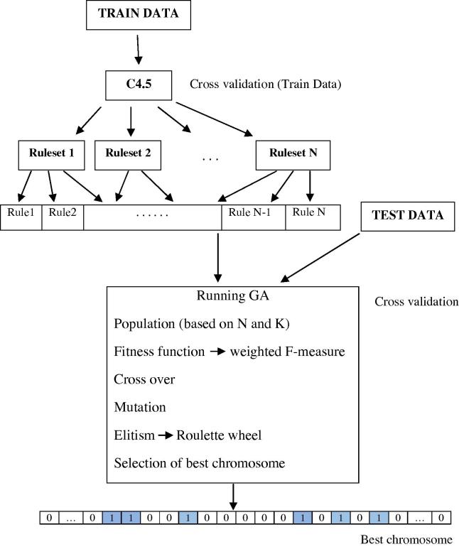
Upon extracting rules, N classification rules are extracted in the form of “if … then …” where N is total of rules in rule sets. Here, the length of chromosome is the number of all rules (N) which is 34 (6 + 9 + 5 + 4 + 6 + 4). Every rule is mapped to a gene, which means the first gene represents the first rule; the second gene represents the second rule and so on. We used a counter, K, rises from 1 to N and represent K randomly selected rules. For example, if K = 5, in all of 34 genes, 5 genes are randomly selected as ‘1’ and the rest considered to be ‘0’. The corresponding’s rule of the genes that equal to 1 will be applied on the dataset and other rules will be ignored. Fig. 1 shows general form of a chromosome. This figure shows 6 rule sets, which have 6, 9, 5, 4, 6 and 4 rules, respectively.

Fig. 1.

General form of a chromosome.

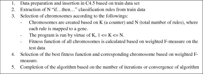
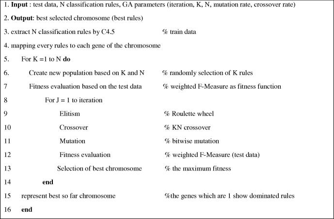
The structure of the proposed algorithm and the pseudo code can be viewed in Fig. 2, Fig. 3, Fig. 4.

Fig. 2.

The proposed method procedure.

Fig. 3.

The schematic representation.

Fig. 4.

Pseudo-code of the proposed method.

2.2.1. Steps

We were able to consider all steps of genetic algorithm. In the first step, the initial population was randomly generated according to the size of K, N. For example, if K = 10 and N = 34, then in randomly initial generated population, in all chromosomes, 10 genes have the value 1 and 24 other genes have value 0 and so on. Then, we calculated the fitness of each chromosome. We used weighted F-measure for fitness evaluation. In doing so, by applying the rules, standing for chromosomes, we were able to calculate how many records could be predicted correctly from the dataset in its corresponding class.

F-measure is a criterion to evaluate the accuracy of classification. For calculation of F-measure, we used two other metrics, which are precision and recall both derived from confusion matrix. Fig. 5 represents confusion matrix [35], [36]. (TP: True Positive; FP: False Positive; FN: False Negative; TN: True Negative).

Fig. 5.

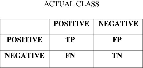
Confusion matrix.

The unique strength point of the present method is the selection of the best measure for comparing the accuracy of classification. The main reason to use weighted F-measure for the fitness function is high difference between instances of each class (imbalance data set). The class 0 has 48 instances whereas the class 1 has 16 instances. We could use another fitness function, which was CCI (correctly classified instances). Because of high difference between the instances in each class, it was a wrong choice of evaluation of the fitness. We show an example to realize the difference between these two criteria (Fig. 6). There are two confusion matrixes, both predict 48 instances correctly (CCI = 48). As depicted, both models have the same CCI, but they have different weighted F-measure. This example emphasizes the strength point of weighted F-measure as a criterion to distinct between different classes in a dataset.

Fig. 6.

Confusion matrix of two models (same CCI and different W-F-measure).

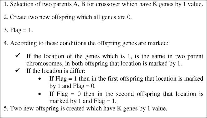
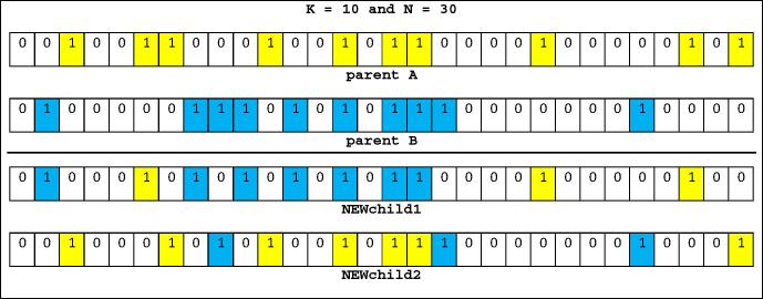
The next step is crossover, which is generation of new children by combination of two parent chromosomes possessing some parent features. The main requirement of crossover operation is having an equal K on both children chromosomes. We named this operation as “KN crossover”, This operation is done based on the crossover rate (P_C). Fig. 7 shows the proposed crossover and Fig. 8 shows two chromosomes and two new children based on the proposed crossover. In this example, K = 10 and N = 30.

Fig. 7.

The proposed “KN crossover”.

Fig. 8.

Two chromosomes and KN crossover.

Mutation operator happens according to mutation rate (P_m), where a gene (or more) with the value 1 transformed into the value of 0 and vice versa. The genes are randomly selected ensuring a new chromosome is created. In this stage, the size of K is preserved as well. After performing above steps, fitness function is calculated for all chromosomes and top populations will be transferred to the next generation by means of roulette wheel. In the last stage, a chromosome with the highest amount of weighted-F-measure is displayed as output. The algorithm can be completed based on the number of iterations or convergence of the algorithm. In the present work, we used the number of iterations. The output of algorithm represents the best possible combination of rules having minimum inconsistency and conflicts.

3. Results and discussion

In our method, we divided the dataset in four folds comprising three folds as training dataset and one fold as the test dataset (48 train samples and 16 test samples). Then, we extracted rules using C4.5 from the training dataset. The extracted rules were applied to the test data and the best rules were selected according to genetic algorithm. This way helps to avoid over fitting and using repetitive data. Consequently, reliable rules can be extracted in this way.

Following extraction of rule sets from training data, we selected the best rules by means of genetic algorithm as follows. First, we explain the parameters of GA in the experiments: roulette wheel selection, KN crossover, bitwise mutation, and elitism are used for performing GA. Also, five parameters need to be adjusted: population size, crossover rate, mutation rate, number of generation, and stopping criterion. The population size, cross over rate, and mutation rate are set to 1000, 0.8, and 0.1, respectively. The genetic algorithm is repeated by 100 generations; the stopping criterion is set to the maximum number of iterations. These parameters are chosen after some trial and error executions.

As mentioned previously, 10-fold cross-validation was used in the previous step (for extracting rules by C4.5 decision tree). In order to avoid over fitting and to extract reliable rules, we used the test dataset. This means that 16 unseen samples were selected and introduced as input to the algorithm. Finally, the best chromosome with the highest possible accuracy was extracted which is shown in Fig. 9. The extracted chromosome indicates that the highest accuracy is achieved when 7 rules are applied on the dataset. As mentioned, the genes (rules) with value equal to 1 have been selected and applied on the dataset and other rules ignored. As appeared in Fig. 9, the extracted rules are 4, 6, 7, 18, 20, 24 and 30. It should be noted that this accuracy was obtained several times during running the proposed method. The confusion matrix of the selected chromosome is also shown in Fig. 10. These rules are defined and presented in Table 7. In this table, correctly predicted instances represents the number of instances which are predicted correctly by each rule alone. This is also true for incorrectly predicted instances. Once all rules applied to the test dataset, the best chromosome was selected in a way to give maximal accuracy, as appeared in Fig. 8, Fig. 9. These figures show that how 93.9 was selected in our trial.

Fig. 9.

The best chromosome.

Fig. 10.

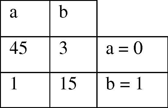
Confusion matrix of the best chromosome.

Table 7.

Extracted rules by the proposed method.

Number of rule	Rule description	Correctly predicted instances	Incorrectly predicted instances
04	if (NonSeed_Energy ⩽ −2.900) && (mRNA_P ⩽ 21) && (max_stem ⩽ 9) && (Seed_paired_pairs > 7)	11	0
prediction = 1
07	if (NonSeed_Energy > −4.400) && (A ⩽ 0.413)	33	2
prediction = 0
15	if (Seed_Energy > −7.100)	17	1
prediction = 0
20	if (NonWC_number > 1) && (Seed_G ⩽ 0.286)	21	0
prediction = 0
21	if (NonSeed_unpaired_bases > 15) && (Seed_G ⩽ 0.286)	7	0
prediction = 0
28	if (mRNA_length > 5.954)	3	0
prediction = 1
30	if (NonSeed_C > 0.312)	6	1
prediction = 0

As appeared, 60 out of 64 samples (45 in class 0 and 15 in class 1) have been selected correctly and there were only 4 incorrect cases which leads us to 0.939 accuracy of prediction. Incorrect cases were the samples 31, 45, 58 and 61 in the presented data set by Yan et al. [16] which is available on http://www.sciencedirect.com/science/article/pii/S0014579307002761#MMCvFirst.

We applied our algorithm to the Yan’s dataset published in 2007 [16]. However, the microRNA/target sites research was in infancy stage by that time, as stage and as many microRNA vs. target sequences were not available. Most recently, many comprehensive databases keeping wider list of validated microRNA/target are available. Therefore, we also used Ahmadi’s dataset published in 2012 [29]. This dataset comprises 425 samples including 312 class 1 and 113 class 0 samples. Besides, it has 12 features that appeared in Table 8. Ahmadi et al. utilized miRNA sequences from miRBase database [37] and downloaded experimentally verified human miRNA targets from TarBase [31] and miRecords [38] databases. Accordingly, the number of branches was 7. The details of the 7 selected rule sets are shown in Table 9 and the selected best rules and their accuracy are appeared in Table 10. We used 319 out of 425 samples as training samples and the rest 106 samples as test samples. The confusion matrix shows that 2 among all class 1 samples and 11 out of 113 class 0 samples have been incorrectly predicted (Fig. 11). Selected chromosome indicates that 7 out of 41 rules have been selected as superior rules (Fig. 12) which are 3, 7, 8, 10, 21, 30 and 41. Therefore, we were able to obtain the same accuracy in both datasets, which confirms high reliability of our method.

Table 8.

Parameters used for miRNA target prediction (Ahmadi et al. data set).

No	Parameter	Parameter description
1	Total score	Obtained by the sum of pair scores. Match + 5, G:U + 1, Mismatch − 3, Gap − 1
2	Seed score	Obtained by the sum of pair scores in the seed region
3	WC pairs	Number of WC pairs in the duplex
4	Wobble pairs	Number of wobble pairs in the duplex
5	Mismatches	Number of mismatches in duplex
6	Number-bulges	Number of bulges in the duplex
7	A proportion	Proportion of “A” in the duplex
8	C proportion	Proportion of “C” in the duplex
9	G proportion	Proportion of “G” in the duplex
10	U proportion	Proportion of “U” in the duplex
11	A:U proportion	Proportion of A:U matches in the duplex
12	Minimum free energy	Calculated using RNAfold for a duplex formed by the miRNA and its target. RNAfold is the part of Vienna RNA package

Adopted from Ahmadi et al. [29].

Table 9.

Details of 7 rule sets.

Rule set	Number of rules	Rule set accuracy on dataset
1	5	88.1
2	7	85.7
3	6	83.33
4	8	90.5
5	6	84.6
6	5	89.2
7	8	91.5

Table 10.

Extracted rules by the proposed method (Ahmadi et al. dataset).

Rule number	Description	Correctly classified instances	Incorrectly classified instances
3	if (Wobble pairs ⩽ 0.217) && (Number-bulges > 0.038)	78	7
prediction = 0;
7	if (Seed score ⩽ 0.967) && (Wobble pairs > 0.217)	293	12
prediction = 1;
8	if (Number-bulges ⩽ 0.080) && (C proportion ⩽ 0.424)	226	20
prediction = 1;
10	if (Total score ⩽ 0.687) && (Seed score > 0.933)	79	21
prediction = 0;
21	if (WC pairs > 0.333) && (Number-bulges > 0.065)	42	1
prediction = 0;
30	if (Wobble pairs > 0.214) && (G proportion > 0.364) && (U proportion > 0.250) && (Minimum free energy > −12.900)	244	1
prediction = 1;
41	if (Number-bulges ⩽ 0.077) && (C proportion > 0.519) && (I > 0.320)	4	0
prediction = 1;

Fig. 11.

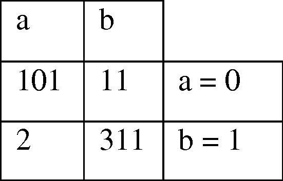
Confusion matrix of best chromosome (Ahmadi et al. dataset).

Fig. 12.

Selected chromosome with highest weighted F-measure.

We compared the proposed method with other methods by WEKA software (Version 3.7.9) [39], [40], [41]. WEKA (http://www.cs.waikato.ac.nz/ml/weka/) is an open source software, which consists of a collection of state-of-the-art machine learning algorithms and data preprocessing tools. It has been developed by the University of Waikato in New Zealand. Written in Java, the WEKA system can be used for a variety of tasks. It provides an implementation of state-of-the-art machine learning algorithms that can be applied to our datasets for extracting information about the data or can be applied to several algorithms in our dataset for comparing their performance.

In this regard, the datasets introduced to WEKA as input. Subsequently, all of the classification algorithms in the software were applied to the datasets. The results are shown in Table 11. This table also depicts the accuracy of our proposed method. It is clear that our proposed method has a much higher accuracy compared to other available classifiers. The higher accuracy can be related to the choice of best rules, which best interact each other.

Table 11.

The classification accuracy of proposed method and other algorithms.

Algorithm	Accuracy (weighted F-measure)
Yan et al. dataset	Ahmadi et al. dataset
BayesNet	0.661	0.918
NaiveBeyes	0.72	0.878
IBK	0.75	0.866
RandomForest	0.775	0.934
RandomTree	0.7	0.915
Bagging	0.73	0.918
AttributeSelection	0.712	0.929
J48	0.731	0.915
RotationForest	0.836	0.928
DecisionTable	0.619	0.924
Adaboost	0.813	0.915
K-NN	0.73	0.908
NBTree	0.861	0.877
SMO	0.658	0.918
SGD	0.737	0.907
Proposed method	0.939	0.971

4. Conclusion

Prediction and validation of miRNA target is costly and time consuming procedure. Machine learning algorithms expedite miRNA target prediction. In doing so, several rules are extracted, which explain the relationships between miRNAs and their targets. Extracted rules, however, have overlaps, incompatibility and incoherence with each other, which make confusion and result in inaccuracy. Our new approach introduced herein increases the classification accuracy of miRNA target prediction. The introduced method was applied on two biologically validated datasets and the results demonstrate the ability and high accuracy of the proposed method.

References

- 1.Carrington J.C., Ambros V. Role of microRNAs in plant and animal development. Science. 2003;301:336–338. doi: 10.1126/science.1085242. [DOI] [PubMed] [Google Scholar]
- 2.Chen X. MicroRNA biogenesis and function in plants. FEBS Lett. 2005;579:5923–5931. doi: 10.1016/j.febslet.2005.07.071. [DOI] [PMC free article] [PubMed] [Google Scholar]
- 3.Zhang B., Pan X., Cannon C.H., Cobb G.P., Anderson T.A. Conservation and divergence of plant microRNA genes. Plant J. 2006;46:243–259. doi: 10.1111/j.1365-313X.2006.02697.x. [DOI] [PubMed] [Google Scholar]
- 4.Lee Y., Ahn C., Han J., Choi H., Kim J., Yim J., Lee J., Provost P., Rådmark O., Kim S. The nuclear RNase III Drosha initiates microRNA processing. Nature. 2003;425:415–419. doi: 10.1038/nature01957. [DOI] [PubMed] [Google Scholar]
- 5.Hutvagner G. Small RNA asymmetry in RNAi: function in RISC assembly and gene regulation. FEBS Lett. 2005;579:5850–5857. doi: 10.1016/j.febslet.2005.08.071. [DOI] [PubMed] [Google Scholar]
- 6.Lim L.P., Lau N.C., Garrett-Engele P., Grimson A., Schelter J.M., Castle J., Bartel D.P., Linsley P.S., Johnson J.M. Microarray analysis shows that some microRNAs downregulate large numbers of target mRNAs. Nature. 2005;433:769–773. doi: 10.1038/nature03315. [DOI] [PubMed] [Google Scholar]
- 7.Pasquinelli A.E. MicroRNAs and their targets: recognition, regulation and an emerging reciprocal relationship. Nat. Rev. Genet. 2012;13:271–282. doi: 10.1038/nrg3162. [DOI] [PubMed] [Google Scholar]
- 8.Lewis B.P., Burge C.B., Bartel D.P. Conserved seed pairing, often flanked by adenosines, indicates that thousands of human genes are microRNA targets. Cell. 2005;120:15–20. doi: 10.1016/j.cell.2004.12.035. [DOI] [PubMed] [Google Scholar]
- 9.Rajewsky N. MicroRNA target predictions in animals. Nat. Genet. 2006;38:S8–S13. doi: 10.1038/ng1798. [DOI] [PubMed] [Google Scholar]
- 10.He L., He X., Lim L.P., De Stanchina E., Xuan Z., Liang Y., Xue W., Zender L., Magnus J., Ridzon D. A microRNA component of the p53 tumour suppressor network. Nature. 2007;447:1130–1134. doi: 10.1038/nature05939. [DOI] [PMC free article] [PubMed] [Google Scholar]
- 11.Carthew R.W., Sontheimer E.J. Origins and mechanisms of miRNAs and siRNAs. Cell. 2009;136:642–655. doi: 10.1016/j.cell.2009.01.035. [DOI] [PMC free article] [PubMed] [Google Scholar]
- 12.Lewis B.P., Shih I.-h., Jones-Rhoades M.W., Bartel D.P., Burge C.B. Prediction of mammalian microRNA targets. Cell. 2003;115:787–798. doi: 10.1016/s0092-8674(03)01018-3. [DOI] [PubMed] [Google Scholar]
- 13.John B., Enright A.J., Aravin A., Tuschl T., Sander C., Marks D.S. Human microRNA targets. PLoS Biol. 2004;2:e363. doi: 10.1371/journal.pbio.0020363. [DOI] [PMC free article] [PubMed] [Google Scholar]
- 14.Krek A., Grün D., Poy M.N., Wolf R., Rosenberg L., Epstein E.J., MacMenamin P., da Piedade I., Gunsalus K.C., Stoffel M. Combinatorial microRNA target predictions. Nat. Genet. 2005;37:495–500. doi: 10.1038/ng1536. [DOI] [PubMed] [Google Scholar]
- 15.Watanabe Y., Yachie N., Numata K., Saito R., Kanai A., Tomita M. Computational analysis of microRNA targets in Caenorhabditis elegans. Gene. 2006;365:2–10. doi: 10.1016/j.gene.2005.09.035. [DOI] [PubMed] [Google Scholar]
- 16.Yan X., Chao T., Tu K., Zhang Y., Xie L., Gong Y., Yuan J., Qiang B., Peng X. Improving the prediction of human microRNA target genes by using ensemble algorithm. FEBS Lett. 2007;581:1587–1593. doi: 10.1016/j.febslet.2007.03.022. [DOI] [PubMed] [Google Scholar]
- 17.Friedman R.C., Farh K.K.-H., Burge C.B., Bartel D.P. Most mammalian mRNAs are conserved targets of microRNAs. Genome Res. 2009;19:92–105. doi: 10.1101/gr.082701.108. [DOI] [PMC free article] [PubMed] [Google Scholar]
- 18.Garcia D.M., Baek D., Shin C., Bell G.W., Grimson A., Bartel D.P. Weak seed-pairing stability and high target-site abundance decrease the proficiency of lsy-6 and other microRNAs. Nat. Struct. Mol. Biol. 2011;18:1139–1146. doi: 10.1038/nsmb.2115. [DOI] [PMC free article] [PubMed] [Google Scholar]
- 19.Enright A.J., John B., Gaul U., Tuschl T., Sander C., Marks D.S. MicroRNA targets in Drosophila. Genome Biol. 2004;5 doi: 10.1186/gb-2003-5-1-r1. R1–R1. [DOI] [PMC free article] [PubMed] [Google Scholar]
- 20.Betel D., Wilson M., Gabow A., Marks D.S., Sander C. The microRNA.org resource: targets and expression. Nucleic Acids Res. 2008;36:D149–D153. doi: 10.1093/nar/gkm995. [DOI] [PMC free article] [PubMed] [Google Scholar]
- 21.Kim S.-K., Nam J.-W., Rhee J.-K., Lee W.-J., Zhang B.-T. MiTarget: microRNA target gene prediction using a support vector machine. BMC Bioinf. 2006;7:411. doi: 10.1186/1471-2105-7-411. [DOI] [PMC free article] [PubMed] [Google Scholar]
- 22.Sheng Y., Engström P.G., Lenhard B. Mammalian microRNA prediction through a support vector machine model of sequence and structure. PloS One. 2007;2:e946. doi: 10.1371/journal.pone.0000946. [DOI] [PMC free article] [PubMed] [Google Scholar]
- 23.Xue C., Li F., He T., Liu G.-P., Li Y., Zhang X. Classification of real and pseudo microRNA precursors using local structure–sequence features and support vector machine. BMC Bioinf. 2005;6:310. doi: 10.1186/1471-2105-6-310. [DOI] [PMC free article] [PubMed] [Google Scholar]
- 24.Yang Y., Wang Y.-P., Li K.-B. MiRTif: a support vector machine-based microRNA target interaction filter. BMC Bioinf. 2008;9:S4. doi: 10.1186/1471-2105-9-S12-S4. [DOI] [PMC free article] [PubMed] [Google Scholar]
- 25.Zhao D., Wang Y., Luo D., Shi X., Wang L., Xu D., Yu J., Liang Y. PMirP: a pre-microRNA prediction method based on structure–sequence hybrid features. Artif. Intell. Med. 2010;49:127–132. doi: 10.1016/j.artmed.2010.03.004. [DOI] [PubMed] [Google Scholar]
- 26.Yousef M., Jung S., Kossenkov A.V., Showe L.C., Showe M.K. Naïve Bayes for microRNA target predictions—machine learning for microRNA targets. Bioinformatics. 2007;23:2987–2992. doi: 10.1093/bioinformatics/btm484. [DOI] [PubMed] [Google Scholar]
- 27.Yousef M., Nebozhyn M., Shatkay H., Kanterakis S., Showe L.C., Showe M.K. Combining multi-species genomic data for microRNA identification using a Naive Bayes classifier. Bioinformatics. 2006;22:1325–1334. doi: 10.1093/bioinformatics/btl094. [DOI] [PubMed] [Google Scholar]
- 28.Chandra V., Girijadevi R., Nair A., Pillai S., Pillai R. MTar: a computational microRNA target prediction architecture for human transcriptome. BMC Bioinf. 2010;11:S2. doi: 10.1186/1471-2105-11-S1-S2. [DOI] [PMC free article] [PubMed] [Google Scholar]
- 29.Ahmadi, H., Ahmadi, A., Azimzadeh-Jamalkandi, S., Shoorehdeli, M.A., Salehzadeh-Yazdi, A., Bidkhori, G., Masoudi-Nejad, A., (2013) HomoTarget: a new algorithm for prediction of microRNA targets in Homo sapiens. Genomics. [DOI] [PubMed]
- 30.Yousef M., Jung S., Showe L.C., Showe M.K. Learning from positive examples when the negative class is undetermined-microRNA gene identification. Algorithms Mol. Biol. 2008;3 doi: 10.1186/1748-7188-3-2. [DOI] [PMC free article] [PubMed] [Google Scholar]
- 31.Sethupathy P., Corda B., Hatzigeorgiou A.G. TarBase: a comprehensive database of experimentally supported animal microRNA targets. RNA. 2006;12:192–197. doi: 10.1261/rna.2239606. [DOI] [PMC free article] [PubMed] [Google Scholar]
- 32.Quinlan J.R. Morgan Kaufmann; 1993. C4. 5: Programs for Machine Learning. [Google Scholar]
- 33.Dreiseitl S., Osl M., Baumgartner C., Vinterbo S. An evaluation of heuristics for rule ranking. Artif. Intell. Med. 2010;50:175–180. doi: 10.1016/j.artmed.2010.03.005. [DOI] [PubMed] [Google Scholar]
- 34.Kohavi, R. (1995) A study of cross-validation and bootstrap for accuracy estimation and model selection. In: Paper Presented at the IJCAI.
- 35.Powers D. Evaluation: from precision, recall and F-measure to roc., informedness, markedness & correlation. J. Mach. Learn. Technol. 2011;2:37–63. [Google Scholar]
- 36.Grossman D.A. Springer; 2004. Information Retrieval: Algorithms and Heuristics. [Google Scholar]
- 37.Griffiths-Jones S., Grocock R.J., Van Dongen S., Bateman A., Enright A.J. MiRBase: microRNA sequences, targets and gene nomenclature. Nucleic Acids Res. 2006;34:D140–D144. doi: 10.1093/nar/gkj112. [DOI] [PMC free article] [PubMed] [Google Scholar]
- 38.Xiao F., Zuo Z., Cai G., Kang S., Gao X., Li T. MiRecords: an integrated resource for microRNA–target interactions. Nucleic Acids Res. 2009;37:D105–D110. doi: 10.1093/nar/gkn851. [DOI] [PMC free article] [PubMed] [Google Scholar]
- 39.Frank E., Hall M., Holmes G., Kirkby R., Pfahringer B., Witten I.H., Trigg L. Springer; 2005. Weka in Data Mining and Knowledge Discovery Handbook; pp. 1305–1314. [Google Scholar]
- 40.Hall M., Frank E., Holmes G., Pfahringer B., Reutemann P., Witten I.H. The WEKA data mining software: an update. ACM SIGKDD Explor. Newsl. 2009;11:10–18. [Google Scholar]
- 41.Frank E., Hall M., Trigg L., Holmes G., Witten I.H. Data mining in bioinformatics using Weka. Bioinformatics. 2004;20:2479–2481. doi: 10.1093/bioinformatics/bth261. [DOI] [PubMed] [Google Scholar]