The shape of terrestrial abundance distributions

Findings of a new, low-dominance distribution of terrestrial abundance: the double geometric.

Abstract

Ecologists widely accept that the distribution of abundances in most communities is fairly flat but heavily dominated by a few species. The reason for this is that species abundances are thought to follow certain theoretical distributions that predict such a pattern. However, previous studies have focused on either a few theoretical distributions or a few empirical distributions. I illustrate abundance patterns in 1055 samples of trees, bats, small terrestrial mammals, birds, lizards, frogs, ants, dung beetles, butterflies, and odonates. Five existing theoretical distributions make inaccurate predictions about the frequencies of the most common species and of the average species, and most of them fit the overall patterns poorly, according to the maximum likelihood–related Kullback-Leibler divergence statistic. Instead, the data support a low-dominance distribution here called the “double geometric.” Depending on the value of its two governing parameters, it may resemble either the geometric series distribution or the lognormal series distribution. However, unlike any other model, it assumes both that richness is finite and that species compete unequally for resources in a two-dimensional niche landscape, which implies that niche breadths are variable and that trait distributions are neither arrayed along a single dimension nor randomly associated. The hypothesis that niche space is multidimensional helps to explain how numerous species can coexist despite interacting strongly.

INTRODUCTION

Counts of individuals grouped into species are a fundamental topic of community ecology because they hint at strong causal factors such as immigration, succession, and competition (1, 2). Modern research on such species abundance distributions stems from a 1932 paper (3) that described the geometric series distribution. This distribution is distinctive because it assumes that species sequentially partition a one-dimensional niche space corresponding with a single resource. Consequently, the abundance of each species is equal to that of the preceding species multiplied by a constant between 0 and 1. Neither the geometric series distribution nor any other distribution that can be derived by assuming competition along a single-niche axis, such as the broken stick model (4), random fraction model (5), power fraction model (6), or stochastic niche model (7), is now widely accepted as describing a large number of communities. On the contrary, it has been claimed that the geometric series distribution is common only in highly disturbed ecosystems (1). The geometric series distribution also seems implausible because it is difficult to imagine how high diversity could be maintained if all species truly competed for a single resource.

Major large-scale studies (8–12) have mostly embraced three other distributions that make different assumptions [for example, (13, 14)]: the lognormal (15), log series (16), and zero-sum multinomial (17, 18). These distributions are much flatter than the geometric series, often with many rare species, but feature high dominance by the most common species. They also assume that species either do not compete with one another asymmetrically or compete along so many niche axes that competition leaves no stamp (1, 18).

This report proposes an entirely different distribution that could be called either the “double geometric” or the “two-dimensional geometric” (Fig. 1A). The double geometric is mathematically related to the geometric series and also assumes niche partitioning. It can be seen as a compromise between the lognormal (Fig. 1B) and the geometric series (Fig. 1C) that makes a very specific prediction about the nature of ecosystems: The success of any species is a function of how it trades off its strategies for capturing resources. Unlike the geometric series and other models, the double geometric model, in its strictest and simplest form, assumes that species compete over exactly two resources (see Materials and Methods). This strong assumption could be relaxed by, for example, allowing for competition in a higher-dimensional niche space. Future research on this topic would be fruitful. However, as is shown here, it is not immediately necessary to make the double geometric more complicated because it already outperforms its rivals.

Fig. 1. Four theoretical abundance distributions fitted, using a consistent criterion (see Materials and Methods), to a data set for bats from Los Tuxtlas Biological Research Station (32), which has exceptionally high species richness and is very well sampled.

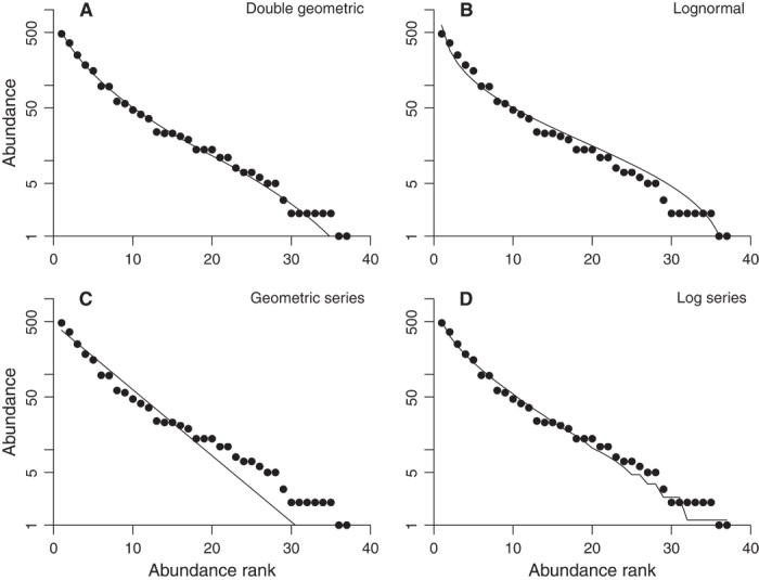
Frequency distribution coverage based on Good’s index [Eq. 8 in (26)] is 0.9990. (A) Double geometric distribution. (B) Lognormal distribution. (C) Geometric series distribution. (D) Log series distribution. The line is jagged at low abundances because predicted values are rounded to the nearest integer.

RESULTS

The major distributions are tested against one another using 1055 community samples of 10 taxonomic groups that are reposed at The Ecological Register (http://ecoregister.org) (see Materials and Methods). Composite rank abundance distributions showing the median relative abundance at each position are remarkably linear across all taxonomic groups (Fig. 2 and fig. S2). Thus, the most common species are less common and the rarest species are less rare than one would expect based on the lognormal (Fig. 1B). Instead, there is only a very subtle upward curvature at the left side, and it is only visible in some cases (for example, tropical trees; birds, ants, and butterflies in general). This curvature is consistent with the modestly high dominance predicted by the double geometric (Fig. 1A). Small drops at the ends of many curves, especially in temperate data, are also consistent with the double geometric. They are certainly not consistent with the geometric series and log series because these two assume there are no detectable limits to the size of the species pool. Although one could argue in an ad hoc way that such limits could be imposed on the geometric series and log series in the real world (that is, that the underlying distributions could be truncated), adding a truncation parameter would render those models less testable.

Fig. 2. Characteristic rank abundance distributions of four disparate taxonomic groups in tropical and temperate zones.

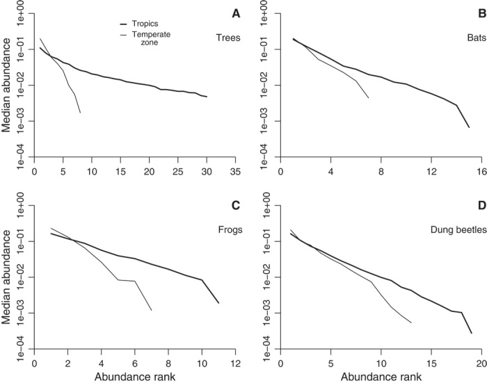
Each value is the median proportional abundance at the appropriate position in the rank abundance distribution. Data are truncated at the point where the median falls to 0. Patterns are similar for the remaining groups (fig. S2). Thick lines, tropical zone data; thin lines, temperate zone data. (A) Trees. (B) Bats. (C) Frogs. (D) Dung beetles.

Understanding the real reasons for the superiority of the double geometric requires considering how the models predict basic aspects of empirical distributions. This report focuses on two: dominance (that is, the proportional abundance of the most common species) and median relative abundance. The first statistic has minimal sampling error and largely governs the observed evenness of a community (1), whereas the second statistic is a very basic descriptor of the entire distribution. Models must be held to predicting such features accurately regardless of how they are parameterized or how well they fit the data in general.

The double geometric model consistently yields accurate estimates of dominance (Fig. 3), as indicated by several statistics (Table 1). First, the estimates and observed values are highly correlated (as with the lognormal and log series but not the geometric series). Second, regression of actual values on double geometric–predicted values produces a slope very close to 1 and an intercept very close to 0. By contrast, the relationship is steep for the lognormal and shallow for the geometric series, whereas the intercepts are much farther from 0 for these two distributions. Although the log series performs better, its intercept is nonetheless substantially farther from 0. The lognormal might appear to perform well upon casual inspection of the data (Fig. 3), but its estimates are consistently too high (Table 1). Finally, the double geometric produces a median offset between predicted and observed values that is considerably smaller than the offsets generated by all other models.

Fig. 3. Predicted and actual dominance (frequency of the most common species) in 1055 ecological samples, including trees (97), bats (159), small terrestrial mammals (161), birds (119), lizards (77), frogs (110), ants (77), dung beetles (115), butterflies (83), and odonates (57).

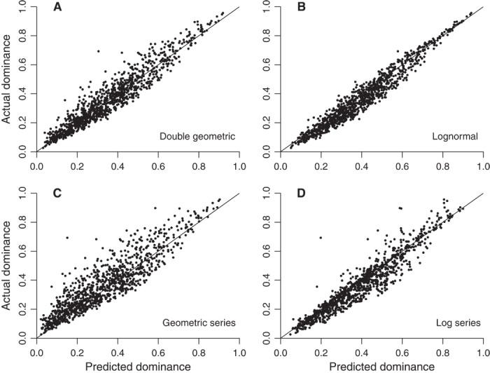
(A) Double geometric distribution. (B) Lognormal distribution. (C) Geometric series distribution. (D) Log series distribution.

Table 1. Regressions of actual dominance on predicted dominance (Fig. 3) and median offsets between actual and predicted dominance based on the fit of six theoretical abundance distributions to the full data set.

The double geometric outperforms all other models with respect to the slope, intercept, and offset.

Distribution	Correlation	Slope	Intercept	Offset
Double geometric	0.9497	0.9940	0.0089	−0.0019
Lognormal	0.9732	1.0327	−0.0439	0.0314
Geometric series	0.9045	0.9214	0.0614	−0.0285
Log series	0.9483	1.0144	−0.0286	0.0162
Broken stick	0.6612	1.0392	0.1260	−0.1044
Zipf	0.9124	1.0764	−0.1520	0.1303

Apart from the double geometric, the models generally perform worse with respect to median abundances (Fig. 4 and Table 2). The lognormal badly overestimates them whereas the geometric series badly underestimates them, as indicated by the median ratios of predicted and observed values. Meanwhile, steep regression slopes indicate that the geometric series and log series substantially compress the range of data and the relationship for the geometric series is patently nonlinear (Fig. 4). By contrast, the double geometric regression for median abundance data produces the one slope that is closest to unity and the one intercept that nearly approaches 0, meaning that the predictions of the double geometric are almost completely accurate.

Fig. 4. Predicted and actual median relative abundances in 1055 ecological samples.

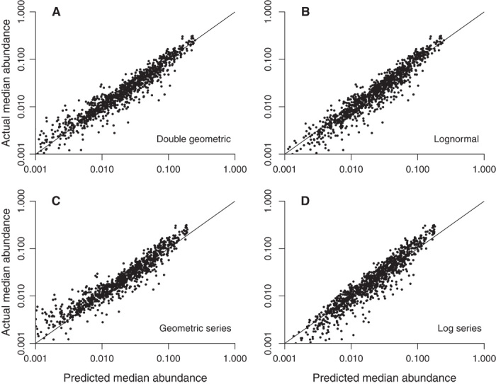
(A) Double geometric distribution. (B) Lognormal distribution. (C) Geometric series distribution. (D) Log series distribution.

Table 2. Regressions of actual median abundance on predicted median abundance (Fig. 4) and median ratios between actual and predicted median abundance based on the fit of six theoretical abundance distributions to the full data set.

The double geometric outperforms all other models with respect to the slope, intercept, and ratio.

Distribution	Correlation	Slope	Intercept	Ratio
Double geometric	0.9496	1.0340	−0.0011	0.9783
Lognormal	0.9473	1.0901	−0.0042	1.0931
Geometric series	0.9442	1.2471	−0.0025	0.8604
Log series	0.9339	1.3473	−0.0062	0.9758
Broken stick	0.7801	0.7689	−0.0089	1.9864
Zipf	0.8885	2.1048	−0.0026	0.5615

The same patterns are seen in subset data for individual groups (figs. S3 to S6). The fit of the double geometric with respect to dominance is consistently impressive (figs. S3 and S4). The double geometric also accurately predicts median abundances in all cases (figs. S5 and S6). Meanwhile, the broken stick is clearly inferior to all of the previously mentioned distributions (fig. S7, A and C, and tables S1 and S2). The Zipf power-law distribution (9, 10) usually overestimates dominance and underestimates median abundance by a substantial margin, and it is arguably the worst of all the alternatives (fig. S7, B and D, and tables S1 and S2).

Another way to distinguish the models is to see how well they predict the overall shapes of rank abundance distributions in a numerical sense. The double geometric, lognormal, and log series models fit the data more or less equally well according to a standard criterion that is related to maximum likelihood (ML) estimation (tables S1 and S2), although the double geometric is significantly better than the log series in several cases (table S3). There is usually a substantial gap between these three models and the others. Because these results are ambiguous, the key evidence in this report is the better fit of the double geometric with respect to dominance and median abundance (Figs. 3 and 4).

DISCUSSION

The double geometric, lognormal, and geometric series models all assume that rank abundance distributions are symmetrical on a log scale: Rare and common species are equally numerous, meaning that underlying rank abundance distributions are neither abruptly truncated nor stretched out by a long tail (Fig. 1). The fact that mean and median abundances in very well sampled distributions closely track each other, especially in high-dominance communities (fig. S8), implies that symmetry is indeed commonplace. Earlier comprehensive analyses also suggested that this pattern is ubiquitous whenever sampling is reasonably complete [for example, (8, 10, 12)], and most evidence to the contrary is limited and focused on high-diversity systems that are intrinsically difficult to sample [for example, (19)]. Nonetheless, a recent large-scale analysis has argued that the inherently skewed and long-tailed log series outperforms the lognormal (11). The current results suggest that the lognormal is marginally better (Tables 1 and 2, tables S1 and S2, and Figs. 3B and 4B versus Figs. 3D and 4D). Regardless, because the data fundamentally support the double geometric, there is every reason to think real-world distributions are indeed symmetrical.

Because the double geometric mandates symmetry and curves at both ends of a rank abundance distribution (Fig. 1 and fig. S1), it should fit poorly to data truncated by undersampling. Indeed, the distributions examined here were not required to have full coverage of the overall species pool. The superior performance of the double geometric in the face of such undersampling suggests both that truncation is usually inconsequential in data sets similar to the ones analyzed here and that the double geometric would best fit even more of the distributions if sampling were better.

Another concern is that different patterns should be seen at different scales (18). This fact works in favor of the double geometric because competition should be more diffuse and niche spaces should be more complex at large scales, making it more difficult to see double geometric–like patterns that might be obvious in more circumscribed samples. Lognormal- or log series–like patterns might be seen instead. Likewise, in unrealistically narrow samples, only one niche axis might be important, creating support for geometric series–like distributions. The fact that the double geometric works so well suggests that ecologists often choose to work at scales that are more meaningful. Additional research on the effects of scale on rank abundance distribution patterns is clearly called for.

The lognormal and log series have been popular in recent literature primarily because no better alternative has been available to date. However, the evidence in favor of these two distributions has been mixed. With a few exceptions (8–12), earlier analyses have been of limited scope [for example, (18–22)]. For example, studies of forest surveys have used either an older broad-brush database that consists of very small samples [for example, (11)] or a handful of large plots [for example, (18–20, 22)]. Recent research has also almost entirely ignored the geometric series, which performs fairly well in predicting median abundances (Fig. 4). One exception was a study showing how the geometric series could be made to approach the lognormal by adding noise (23), which is a moot point both because the double geometric can be made to resemble either distribution and because the data decisively reject the geometric series. Instead, the literature has generally focused on various models that predict lognormal-, log series–, or zero-sum multinomial–like patterns [for example, (8, 11, 12, 18, 19)] or even a combination of the lognormal and log series (21). Two research groups also looked at the Zipf (9, 10) and another group looked at the broken stick (22), but only one of them (9) also considered the geometric series. As for the zero-sum multinomial (18) and related models, they are not explored here in detail for technical reasons (see Materials and Methods). Regardless, there is no reason to believe they fit real distributions any better than do the lognormal or log series (9, 12) and they variously predict lognormal-, log series–, and geometric series–like patterns rejected by current data (tables S1 and S2). Finally, the stochastic niche model predicts highly skewed distributions that generally resemble either the broken stick or a truncated geometric series (7); thus, it can be put aside.

A certain amount of chaos in the literature has been suggested by the previous discussion, and some do argue that the situation has reached an impasse (2). If so, then testing additional predictions of models that go beyond the shape of rank abundance distributions is the only recourse (2). However, it seems that discriminating models is relatively straightforward (Figs. 3 and 4, fig. S7, and Tables 1 and 2). Thus, it makes the most sense to focus on the data that all of these models were developed to address: the shapes of abundance distributions.

In sum, patterns in most terrestrial communities are best explained by a model whose formulation invokes strong competition and does so in a very specific way. Relaxing the model’s assumptions that only two axes are important and that they are equally important would strengthen its explanatory power even further. By contrast, the laissez-faire scenarios of the lognormal and log series, which in most formulations assume that competition is weak, absent, or overridden by random chance (1), receive no strong empirical support in this study (tables S1 to S3 and Figs. 3 and 4). The geometric series does invoke strong competition but only makes sense when diversity is low and it fits the data very poorly (tables S1 and S2, and Figs. 3C and 4C versus Figs. 3B and 4B). Specifically, it fails to explain why common species are so common. The double geometric does.

The empirical results have implications that go far beyond a theoretical dispute about distribution shapes. For example, because the double geometric implies that niche segregation is mostly confined to two or perhaps a few axes, trait distributions in communities should be neither completely independent nor tightly correlated to form a single gradient. It implies that niche breadths are not uniform because some species are superior competitors. Like the lognormal, and unlike many other models, it implies that most local communities have well-circumscribed, knowable, and finite levels of species richness. Meanwhile, acceptance of the double geometric would challenge the use of Fisher’s α as a measure of diversity because it is the governing parameter of the log series. The double geometric would also raise serious questions about the use of Shannon’s H in the same role because of that index’s rather intimate connection to the lognormal (1, 24).

Most importantly, this study suggests a mechanism that may help to account for one of the most fundamental dilemmas in ecology: How can hundreds or even thousands of related species coexist regionally on evolutionary time scales given that they consume the same limited resources? In other words, how can competition and high diversity be squared with each other? The most parsimonious solution is to assume that competition has very real effects but that niches are distributed in a large low-dimensional landscape (25), allowing a multiplicity of forms to survive by trading off their ecological investments.

MATERIALS AND METHODS

Data were compiled record by record from the primary literature and entered into The Ecological Register (http://ecoregister.org). All records were contributed by the author, although some were keystroked by an assistant before being vetted. Samples were only accepted if the authors reported abundances for all species they encountered. Composite abundances representing multiple sampling localities were accepted. Only absolute counts, as opposed to relative proportions, were considered. In general, when a paper reported more than three samples from the same coordinate representing the same habitat, only the first sample was entered in the database. However, the tree data set includes almost all published samples. Regardless, whenever replicates existed, only the largest sample was downloaded and used in the analyses. Samples from small oceanic islands and urban areas were excluded. Tree samples from cropland, pasture, plantation, disturbed forest, and suburban settings were also omitted, and tree samples were required to employ a minimum diameter at breast height (DBH) cutoff of 9.09 to 11 cm; most had a 10-cm minimum DBH. Dung beetle and ant data were almost entirely based on pitfall or Winkler trap samples; butterfly data mostly stemmed either from baited trap samples or from visual censuses; odonate sampling variously involved sieves, nets, hand captures, and visual censuses; frog and lizard data mostly stemmed from hand captures; small mammal data were based on trapping surveys; and bird and bat data were based almost entirely on mist net samples. Samples were required to include between 50 and 10,000 individuals and to present a frequency distribution coverage of 0.90, as indicated by Good’s index [Eq. 8 in (26)]. Use of the latter cutoff had hardly any effect on the analysis because most samples in the database already exceeded it.

The double geometric model can be explained as follows. Let κ be a constant analogous to the geometric series niche preemption coefficient (3), but assume that (i) there is a fixed number of species S such that the underlying distribution is truncated, and (ii) each species takes a separate position in the community at a coordinate on two orthogonal niche partitioning axes. The axes do not represent the actual value of a resource; instead, they represent the order of preemption, which generates particular apportionment sizes. Likewise, the ordering has to do with relative adaptive success and has nothing to do with the literal temporal sequence in which species invade a particular habitat, although a mechanistic model making such an assumption could be developed [as in (7)].

As with the geometric series, resource apportionment to the ith species on the first axis scales to κ(1 − κ)^i−l (1, 3). Apportionment to the most common species (that is, dominance) is just κ. If a given species takes the ith position on one axis and the jth on the other, its abundance can be modeled as the product of apportionments κ(1 − κ)^i−lκ(1 − κ)^j−l divided by the sum of all such products. Another form of the equation is ${\mathrm{\kappa }}^2{(1-\mathrm{\kappa })}^{\mathit{i}+\mathit{j}-2}$ . The sum i + j has a triangular distribution much akin to the probability of obtaining a number by throwing two dice, each with S surfaces, such that the chance of obtaining the maximum possible resource apportionment is 1/S² and that of obtaining the modal apportionment is 1/S.

Note that κ is assumed to be the same on both axes, meaning that resources are distributed with the same evenness and that κ is near 0 (but not 0) for the other axes (meaning that they are unconnected to abundance because resources on these axes are effectively unlimited). This strong assumption could be relaxed, but doing so would require adding more free parameters and thus would make the model less testable. It also might cause the double geometric to limit on the lognormal. At the same time, if κ were near 0 for all axes save the first, then one would arrive back at the geometric series, which again is rejected by the data.

It is true that high-dimensional niche axes must play a role in structuring communities, and it is an intentional simplification to assume that the first two are equally important. In the real world, it is likely that the κ parameters for different axes trail off following a distribution that might or might not be steep, depending on the community at hand. For example, κ might fall off exponentially in a series such as 0.1, 0.05, 0.025… . This very real possibility makes it obvious that varying the number of axes and varying κ among axes would be a worthwhile avenue for future research. Nonetheless, simple and strongly testable models that explain the data well are to be preferred on both practical and philosophical grounds.

The double geometric distribution of apportionments can be easily computed by numerical simulation and produces symmetrical rank abundances in the same way that the lognormal does (that is, long tails are absent and curves are not abruptly truncated; Fig. 1, A versus B). The difference is that the double geometric can predict straight line patterns just about as well as the geometric series when there is no high dominance (fig. S1).

No analytical solution for the double geometric distribution exists. However, a fair approximation is to estimate the rth abundance in a single series (that is, a rank abundance distribution) as the preceding abundance multiplied by a constant, as with the geometric series. The estimate for the first species is set to κ and the constant is ${\mathrm{\kappa }}^{1/\sqrt{\mathit{x}}}$, where x is the minimum of r/S and (S − r + 1)/S. After being computed, the values are divided by their sum so that they will add up to 1. It seems likely that a proof will be found to show that the general equation κ²(1 − κ)^{i + j − 2} (in which i and j are positions on niche axes) can be collapsed into ${\mathrm{\kappa }}^{1/\sqrt{\mathit{x}}}$ (in which r is a position in a rank abundance distribution).

A single criterion was used to fit each of the models, namely, minimizing the Kullback-Leibler (K-L) divergence statistic. This widely used equation is the sum of the products p_r log(p_r/q_r) where p_r is the observed frequency of species r in the rank abundance distribution and q_r is the estimated frequency. It is analogous to the Shannon index: ln S − H is the divergence between the observed data and a uniform distribution. Minimizing divergence is equivalent to maximizing the log likelihood of the data given the hypothesized distribution (27). Because rare species have low frequencies, they contribute little to the statistic, and models are therefore only lightly penalized for hypothesizing unsampled rare species on the theory that distributions are truncated. In each distribution’s case, either an exhaustive enumeration or a simple hill-climbing algorithm was used to optimize the free parameters.

It would be tempting to take a pure ML or Bayesian approach (22, 24, 28) instead of working with the K-L statistic. Unfortunately, such methods are not available for every distribution. An example is the geometric series, perhaps because it has been paid limited attention by theorists in recent years. In addition, ML and Bayesian fitting would be computationally prohibitive in some cases given the size of the data set. The relatively fast and simple K-L fitting procedure was therefore used instead. The details are as follows:

1) As previously mentioned, the double geometric can be fitted by simulation. Unfortunately, this method is far too slow when dealing with hundreds of samples. Instead, fitting was based on the approximate equation. A search over the range S′ = S to 10S and κ = 0 to κ = 1 was carried out. S′ is the optimized species pool size. κ was varied by a hill-climbing algorithm in which a small normally distributed random number was added to the best-so-far value at each step and the derived figure was accepted if it improved the K-L fit. One hundred values were examined each time S′ was incremented.

2) The underlying parameters of the lognormal are best fitted by assuming that the abundances are Poisson-distributed (24) and by computing the mean μ and SD σ either by ML optimization (24, 28) or by Bayesian inference (22). The latter approach is not feasible here for computational reasons. More importantly, comparisons must be made on a level playing field; therefore, a fitting method using the K-L criterion must be used. The point of the exercise is to test whether the lognormal has strong explanatory power, not to find the optimal underlying parameters; thus, using uniform criteria is imperative. Therefore, I have implemented a K-L fitting routine that optimizes S′ and σ instead of μ and σ. Taking this approach allows predicting an exact relative abundance at each rank in the realized community’s rank abundance distribution (where the “realized community” is the set of species actually living in a place at a point in time). S′ is implied by μ because this parameter identifies median-rank species. For example, if this species is at position 10, then there should be 19 species in the realized species pool, although some might be missed because of undersampling. As in the case of the double geometric, I have varied S′ from S to 10S and have optimized σ by hill-climbing. Abundances are then easily computable by translating species ranks into quantiles and by then converting quantiles into densities. The R function qnorm was used for this purpose. For example, if S′ = 20 and σ = 2, then the logged abundance of the first species is qnorm(0.975,sd=2) and that of the second is qnorm(0.925,sd=2). The resulting values were then exponentiated and divided by their sum to obtain relative frequencies.

3) Several methods, all of them simple, are used to fit the geometric series governing parameter k (1, 29). Here I obtained the starting values of k using a routine linear regression approach in which logged abundances are regressed on ranks. The parameter k was then equated with the slope. The only twist on this approach is that the frequencies were weighted by their square roots to minimize the effects of random counting error. Another hill-climbing algorithm was then used to optimize k, which means that the regression step was only used to speed up the solution.

4) The governing parameter α of the log series distribution is conventionally and easily fitted using a recursive equation (1) that relates α to the numbers of species S and to the number of individuals N. This equation was used to obtain a starting value only. The parameter α was then optimized by hill-climbing, which means it was free to explain the data as well as possible. Unfortunately, the log series predicts the number of species S_x with a given count x, instead of the expected count N_r of the species having rank r, in a rank abundance distribution. A trivial method was used to convert one into the other. (a) A cumulative distribution of S_x across possible counts was computed. (b) The distribution was examined one step at a time, and a break point was found where the rounded number of species predicted to have x or less was greater than the rounded number predicted to have x − 1 or less. (c) The difference between the rounded values y was stored. (d) y species were declared to have the abundance x and were added to the rank abundance distribution. (e) Steps (b) to (d) were iterated until the rank abundance distribution was filled.

5) The only parameter of the broken stick distribution (4) is S′, which is the number of species in the sampling pool. The computation itself is straightforward (1). An exhaustive search over the range S to 3S was used to optimize S′.

6) Being based on a simple power-law relationship, the only free parameter of the Zipf distribution is the slope of a curve relating the log of abundance to the log of rank. The initial slope was fitted by a routine linear regression with points weighted by the square root of absolute abundance (for reasons given previously). The predicted values were divided by their sum to obtain relative frequencies. The slope was then optimized by hill-climbing.

Although several distributions, including the log series, can be fitted to data without any optimization, note that all of them actually were optimized. Thus, the K-L comparisons honestly do rest on a level playing field.

The zero-sum multinomial distribution (17, 18) could not be explored for a simple technical reason: There is no clear way to fit it to a rank abundance distribution using the K-L divergence statistic, and fitting it using another criterion would create an apples-and-oranges comparison. In addition, there are so many model variants that choosing how to test the zero-sum multinomial becomes a matter of taste (19, 20, 22). Although an approximation to the basic form of the zero-sum multinomial could have been used instead (12), there are other good reasons to table the issue: (a) the zero-sum multinomial limits on the log series when diversity is low (17, 18) and the geometric series when it is high (17, 18), but both models are decisively rejected by the data [Tables 1 and 2 and Figs. 3 and 4; see also (8)]; (b) when diversity is intermediate, the rank abundance distribution should resemble the highly skewed broken stick distribution [figs. 5.1 and 5.2 in (18)], which is almost the worst model of any tested here (Tables 1 and 2, tables S1 and S2, and fig. S7); and (c) earlier comprehensive studies have already shown the lognormal to fit real data better than does the zero-sum multinomial (9, 12).

The second point deserves some elaboration. Given a skewed distribution such as the broken stick, the mean abundance on a log scale should be less than the median abundance. However, the means and medians in the 10 current data sets show the opposite relationship when both measures are low (fig. S8). This pattern could have resulted from undersampling (the cutoff for inclusion in the figure is u = 0.99 or better, a high but not exceptionally high threshold) or from the approach of the individual distributions toward the log series. However, regardless of the average value of the mean, the average median is the same or lower. Thus, again, the zero-sum multinomial is not tenable because it predicts various shapes resembling three different distributions that are all inconsistent with actual data.

Other more obscure models that also assume ecological equivalence between species make predictions similar to those of the zero-sum multinomial. These tend to generate unrealistically skewed distributions of abundances and either invoke a composition of multiple distinct underlying distributions (21) or assume that communities are out of equilibrium and that most species are slowly spiraling toward extinction (30). Either assumption would seem to be unparsimonious: it is far more simple to posit that a single mechanism has generated each distribution and that local communities are in equilibrium.

The power fraction model (6) could not be included in this study because there is no means of fitting it precisely to individual distributions. This model includes the broken stick as a special case. It seems to be less than plausible because, similar to the stochastic niche model (7), it implies very low dominance and therefore produces distributions that often resemble not only the widely rejected broken stick distribution but also the poorly supported geometric series distribution (31).

A key argument here is that the double geometric outperforms the conceptually related lognormal, which creates similar distributions (Fig. 1 and fig. S1) and is favored in the literature [for example, (8–12)]. The margin between the two with respect to overall fit is very narrow (tables S1 to S3), although the double geometric is much better with respect to dominance and median abundance prediction (Tables 1 and 2 and Figs. 3 and 4). Furthermore, the lognormal consistently outperforms other models (Tables 1 and 2 and tables S1 and S2). Thus, it is particularly important to explain that the differential between the double geometric and the lognormal is unlikely to be an artifact of some kind. Reasons for believing this claim are as follows:

1) As with the log series, the lognormal has been fitted just as carefully as the double geometric using a similar hill-climbing algorithm.

2) The K-L approach is specifically designed to match the rank abundance distribution using an ML-based criterion. Although other methods (12, 22, 24) might do a better job of revealing the true values of the underlying parameters of the lognormal, this does not mean that they should do a better job of fitting the rank abundance distribution per se.

3) Undersampling that leads to truncation of rank abundance distributions would obscure double geometric patterns, not only lognormal patterns, by creating the impression that rare species are common (when both models posit that they are rare). Thus, this factor is unlikely to explain the superior performance of the double geometric.

4) Finally, it is impossible to square the lognormal with the median curve shape patterns (Fig. 2 and fig. S2), which are easily predicted by the double geometric (Fig. 1 and fig. S1).

To sum up, because well-sampled real-world distributions tend to be symmetrical and tend not to have long tails (Fig. 1 and fig. S1), the lognormal seems to be the most viable alternative to the double geometric. However, it is very difficult to see how its inferior performance (Tables 1 and 2) could be explained as being some kind of error or artifact. It falls on advocates of the lognormal to explain why this model should be accepted in the absence of clear empirical support for it.

SUPPLEMENTARY MATERIALS

Supplementary material for this article is available at http://advances.sciencemag.org/cgi/content/full/1/8/e1500082/DC1

Fig. S1. Four theoretical abundance distributions fitted to a data set for birds from Poland (33), which has the highest species richness of any complete sample for this group included in this analysis.

Fig. S2. Characteristic rank abundance distributions of six additional taxonomic groups in tropical and temperate zones based on Fig. 2.

Fig. S3. Predicted and actual dominance in four disparate groups based on the double geometric distribution.

Fig. S4. Predicted and actual dominance in six additional groups based on the double geometric distribution.

Fig. S5. Predicted and actual median relative abundances in four disparate groups based on the double geometric distribution.

Fig. S6. Predicted and actual median relative abundances in six additional groups based on the double geometric distribution.

Fig. S7. Predicted and actual dominance and median relative abundance based on the broken stick and Zipf distributions.

Fig. S8. Mean and median abundances observed in relatively well-sampled distributions.

Table S1. Medians of the fit of the six theoretical abundance distributions to observed frequencies as measured by K-L divergence statistics.

Table S2. Means of the fit of the six theoretical abundance distributions to observed frequencies.

Table S3. Results of tests for differences between distributions of K-L divergence statistics.

Appendix S1. R code used to perform the analyses.

Reference (33)

REFERENCES AND NOTES

- 1.R. M. May, in Ecology and Evolution of Communities, M. L. Cody, J. M. Diamond, Eds. (Belknap, Cambridge, MA, 1975), pp. 81–120. [Google Scholar]
- 2.McGill B. J., Etienne R. S., Gray J. S., Alonso D., Anderson M. J., Benecha H. K., Dornelas M., Enquist B. J., Green J. L., He F., Hurlbert A. H., Magurran A. E., Marquet P. A., Maurer B. A., Ostling A., Soykan C. U., Ugland K. I., White E. P., Species abundance distributions: Moving beyond single prediction theories to integration within an ecological framework. Ecol. Lett. 10, 995–1015 (2007). [DOI] [PubMed] [Google Scholar]
- 3.Motomura I., A statistical treatment of associations. Jap. J. Zool. 44, 379–383 (1932). [Google Scholar]
- 4.MacArthur R., On the relative abundance of bird species. Proc. Natl. Acad. Sci. U.S.A. 43, 293–295 (1957). [DOI] [PMC free article] [PubMed] [Google Scholar]
- 5.Tokeshi M., Niche apportionment or random assortment: Species abundance patterns revisited. J. Anim. Ecol. 59, 1129–1146. (1990). [Google Scholar]
- 6.Tokeshi M., Power fraction: A new explanation of relative abundance patterns in species-rich assemblages. Oikos 75, 543–550 (1996). [Google Scholar]
- 7.Tilman D., Niche tradeoffs, neutrality, and community structure: A stochastic theory of resource competition, invasion, and community assembly. Proc. Natl. Acad. Sci. U.S.A. 101, 10854–10861 (2004). [DOI] [PMC free article] [PubMed] [Google Scholar]
- 8.Connolly S. R., Hughes T. P., Bellwood D. R., Karlson R. H., Community structure of corals and reef fishes at multiple scales. Science 309, 1363–1365 (2005). [DOI] [PubMed] [Google Scholar]
- 9.Wagner P. J., Kosnik M. A., Lidgard S., Abundance distributions imply elevated complexity of post-Paleozoic marine ecosystems. Science 314, 1289–1292 (2006). [DOI] [PubMed] [Google Scholar]
- 10.Ulrich W., Ollik M., Ugland K. I., A meta-analysis of species–abundance distributions. Oikos 119, 1149–1155 (2010). [Google Scholar]
- 11.White E. P., Thibault K. M., Xiao X., Characterizing species abundance distributions across taxa and ecosystems using a simple maximum entropy model. Ecology 93, 1772–1778 (2012). [DOI] [PubMed] [Google Scholar]
- 12.Connolly S. R., MacNeil M. A., Caley M. J., Knowlton N., Cripps E., Hisano M., Thibaut L. M., Bhattacharya B. D., Benedetti-Cecchi L., Brainard R. E., Brandt A., Bulleri F., Ellingsen K. E., Kaiser S., Kröncke I., Linse K., Maggi E., O’Hara T. D., Plaisance L., Poore G. C., Sarkar S. K., Satpathy K. K., Schückel U., Williams A., Wilson R. S., Commonness and rarity in the marine biosphere. Proc. Natl. Acad. Sci. U.S.A. 111, 8524–8529 (2014). [DOI] [PMC free article] [PubMed] [Google Scholar]
- 13.Pueyo S., He F., Zillio T., The maximum entropy formalism and the idiosyncratic theory of biodiversity. Ecol. Lett. 10, 1017–1028 (2007). [DOI] [PMC free article] [PubMed] [Google Scholar]
- 14.Harte J., Zillio T., Conlisk E., Smith A. B., Maximum entropy and the state-variable approach to macroecology. Ecology 89, 2700–2711 (2008). [DOI] [PubMed] [Google Scholar]
- 15.Preston F. W., The canonical distribution of commonness and rarity: Part I. Ecology 43, 185–215 (1962). [Google Scholar]
- 16.Fisher R. A., Corbet A. S., Williams C. B., The relation between the number of species and the number of individuals in a random sample of an animal population. J. Anim. Ecol. 12, 42–58 (1943). [Google Scholar]
- 17.Caswell H., Community structure: A neutral model analysis. Ecol. Monogr. 46, 327–354 (1976). [Google Scholar]
- 18.S. P. Hubbell, The Unified Theory of Biogeography and Biodiversity (Princeton University Press, Princeton, NJ, 2001). [Google Scholar]
- 19.Volkov I., Banavar J. R., He F., Hubbell S. P., Maritan A., Density dependence explains tree species abundance and diversity in tropical forests. Nature 438, 658–661 (2005). [DOI] [PubMed] [Google Scholar]
- 20.Chave J., Alonso D., Etienne R. S., Theoretical biology: Comparing models of species abundance. Nature 441, E1 (2006). [DOI] [PubMed] [Google Scholar]
- 21.Magurran A. E., Henderson P. A., Explaining the excess of rare species in natural species abundance distributions. Nature 422, 714–716 (2003). [DOI] [PubMed] [Google Scholar]
- 22.Etienne R. S., Olff H., Confronting different models of community structure to species-abundance data: A Bayesian model comparison. Ecol. Lett. 8, 493–504 (2005). [DOI] [PubMed] [Google Scholar]
- 23.Loehle C., Species abundance distributions result from body size–energetics relationships. Ecology 87, 2221–2226 (2006). [DOI] [PubMed] [Google Scholar]
- 24.Bulmer M. G., On fitting the Poisson lognormal distribution to species-abundance data. Biometrics 30, 101–110 (1974). [Google Scholar]
- 25.Valentine J. W., Determinants of diversity in higher taxonomic categories. Paleobiology 6, 444–450 (1980). [Google Scholar]
- 26.Good I. J., The population frequencies of species and the estimation of population parameters. Biometrika 40, 237–264 (1953). [Google Scholar]
- 27.J. Shlens, Notes on Kullback-Leibler divergence and likelihood. arXiv:1404.2000v1 [ci.IT] (2014).
- 28.Engen S., Lande R., Walla T., DeVries P. J., Analyzing spatial structure of communities using the two-dimensional Poisson lognormal species abundance model. Am. Nat. 160, 60–73 (2002). [DOI] [PubMed] [Google Scholar]
- 29.He F., Tang D., Estimating the niche preemption parameter of the geometric series. Acta Oecol. 33, 105–107 (2008). [Google Scholar]
- 30.P. A. Marquet, J. E. Keymer, H. Cofré, in Macroecology: Concepts and Consequences, K. H. Gaston, T. M. Blackburn, Eds. (Blackwell Science, Oxford, UK, 2003), pp. 64–84. [Google Scholar]
- 31.Ferreira F. C., Petrere M. Jr, Comments about some species abundance patterns: Classic, neutral, and niche partitioning models. Braz. J. Biol. 68, 1003–1012 (2008). [DOI] [PubMed] [Google Scholar]
- 32.Estrada A., Coates-Estrada R., Species composition and reproductive phenology of bats in a tropical landscape at Los Tuxtlas, Mexico. J. Trop. Ecol. 17, 627–646 (2001). [Google Scholar]
- 33.Dolnik O. V., Dolnik V. R., Bairlein F., The effect of host foraging ecology on the prevalence and intensity of coccidian infection in wild passerine birds. Ardea 98, 97–103 (2010). [Google Scholar]
Associated Data
This section collects any data citations, data availability statements, or supplementary materials included in this article.