Dynamic Cascades with Bidirectional Bootstrapping for Action Unit Detection in Spontaneous Facial Behavior

Abstract

Automatic facial action unit detection from video is a long-standing problem in facial expression analysis. Research has focused on registration, choice of features, and classifiers. A relatively neglected problem is the choice of training images. Nearly all previous work uses one or the other of two standard approaches. One approach assigns peak frames to the positive class and frames associated with other actions to the negative class. This approach maximizes differences between positive and negative classes, but results in a large imbalance between them, especially for infrequent AUs. The other approach reduces imbalance in class membership by including all target frames from onsets to offsets in the positive class. However, because frames near onsets and offsets often differ little from those that precede them, this approach can dramatically increase false positives. We propose a novel alternative, dynamic cascades with bidirectional bootstrapping (DCBB), to select training samples. Using an iterative approach, DCBB optimally selects positive and negative samples in the training data. Using Cascade Adaboost as basic classifier, DCBB exploits the advantages of feature selection, efficiency, and robustness of Cascade Adaboost. To provide a real-world test, we used the RU-FACS (a.k.a. M3) database of nonposed behavior recorded during interviews. For most tested action units, DCBB improved AU detection relative to alternative approaches.

1 Introduction

The face is one of the most powerful channels of nonverbal communication. Facial expression provides cues about emotional response, regulates interpersonal behavior, and communicates aspects of psychopathology. To make use of the information afforded by facial expression, Ekman and Friesen [1] proposed the Facial Action Coding System (FACS). FACS segments the visible effects of facial muscle activation into “action units (AUs).” Each action unit is related to one or more facial muscles. These anatomic units may be combined to represent more molar facial expressions. Emotion-specified joy, for instance, is represented by the combination of AU6 (cheek raiser, which results from contraction of the orbicularis occuli muscle) and AU12 (lip-corner puller, which results from contraction of the zygomatic major muscle). The FACS taxonomy was developed by manually observing live and recorded facial behavior and by recording the electrical activity of underlying facial muscles [2]. Because of its descriptive power, FACS has become the state of the art in manual measurement of facial expression [3] and is widely used in studies of spontaneous facial behavior [4]. For these and related reasons, much effort in automatic facial image analysis seeks to automatically recognize FACS action units [5], [6], [7], [8], [9].

Automatic detection of AUs from video is a challenging problem for several reasons. Nonfrontal pose and moderate to large head motion make facial image registration difficult, large variability occurs in the temporal scale of facial gestures, individual differences occur in shape and appearance of facial features, many facial actions are inherently subtle, and the number of possible combinations of 40+ individual action units numbers in the thousands. More than 7,000 action unit combinations have been observed [4]. Previous efforts at AU detection have emphasized types of features and classifiers. Features have included shape and various appearance features, such as grayscale pixels, edges, and appearance (e.g., canonical appearance, Gabor, and SIFT descriptors). Classifiers have included support vector machines (SVM) [10], boosting [11], hidden Markov models (HMM) [12], and dynamic Bayesian networks (DBN) [13] review much of this literature.

By contrast, little attention has been paid to the assignment of video frames to positive and negative classes. Typically, assignment has been done in one of two ways. One assigns to the positive class those frames at the peak of each AU or proximal to it. Peak refers to frame of maximum intensity of an action unit between when it begins (“onset”) and when it ends (“offset”). The negative class then is chosen by randomly sampling other AUs, including AU 0 or neutral. This approach suffers at least two drawbacks: 1) The number of training examples will often be small, which results in a large imbalance between positive and negative frames, and 2) peak frames may provide too little variability to achieve good generalization. These problems may be circumvented by following an alternative approach, that is, to include all frames from onset to offset in the positive class. This approach improves the ratio of positive to negative frames and increases the representativeness of positive examples. The downside is confusability of positive and negative classes. Onset and offset frames and many of those proximal or even further from them may be indistinguisable from the negative class. As a consequence, the number of false positives can dramatically increase.

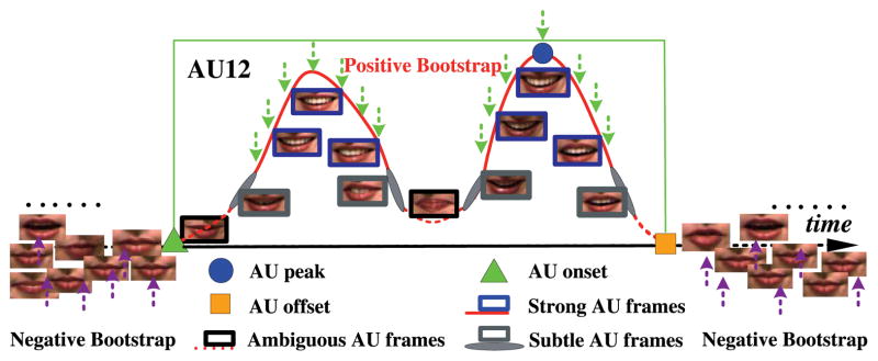
To address these issues, we propose an extension of Adaboost [14], [15], [16] called Dynamic Cascades with Bidirectional Bootstrapping (DCBB). Fig. 1 illustrates the main idea. Having manually annotated FACS data with onset, peak, and offset, the question we address is how best to select the AU frames for the positive and negative class. Preliminary results for this work has been presented in [17].

Fig. 1.

Example of strong, subtle, and ambiguous samples of FACS action unit 12. Strong samples typically correspond to the peak, or maximum intensity, and ambiguous frames correspond to AU onset and offset and frames proximal to them. Subtle samples are located between strong and ambiguous ones. Using an iterative algorithm, DCBB selects positive samples such that the detection accuracy is optimized during training.

In contrast to previous approaches to class assignment, DCBB automatically distinguishes between strong, subtle, and ambiguous frames for AU events of different intensity. Strong frames correspond to the peaks and the ones proximal to them; ambiguous frames are proximal to onsets and offsets; subtle frames occur between strong and ambiguous ones. Strong and subtle frames are assigned to the positive class. By distinguishing between these three types, DCBB maximizes the number of positive frames while reducing confusability between positive and negative classes.

For high intensity AUs in comparison with low intensity AUs, the algorithm will select more frames for the positive class. Some of these frames may be similar in intensity to low intensity AUs. Similarly, if multiple peaks occur between an onset and offset, DCBB assigns multiple segments to the positive class. See Fig. 1 for an example. Strong and subtle, but not ambiguous AU frames are assigned to the positive class. For the negative class, DCBB proposes a mechanism which is similar to Cascade AdaBoost to optimize that as well; the principles are that the weight of misclassified negative class will be increased during training step of each weak classifier and do not learn too much at each cascade stage. Moreover, the positive class is changed at each iteration, while the corresponding negative class is reselected again.

In experiments, we evaluated the validity of our approach to class assignment and selection of features. In the first experiment, we illustrate the importance of selecting the right positive samples for action unit detection. In the second, we compare DCBB with standard approaches based on SVM and AdaBoost.

The rest of the paper is organized as follows: Section 2 reviews previous work on automatic methods for action unit detection. Section 3 describes preprocessing steps for alignment and feature extraction. Section 4 gives details of our proposed DCBB method. Section 5 provides experimental results in nonposed, naturalistic video. For experimental evaluation, we used FACS-coded interviews from the RU-FACS (a.k.a. M3) database [18], [19]. For most action units tested, DCBB outperformed alternative approaches.

2 Previous Work

This section describes previous work on FACS and on automatic detection of AUs from video.

2.1 FACS

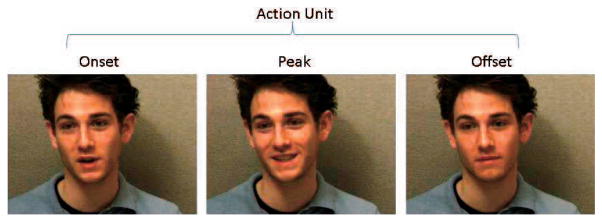
The FACS [1] is a comprehensive, anatomically-based system for measuring nearly all visually discernible facial movement. FACS describes facial activity on the basis of 44 unique action units (AUs), as well as several categories of head and eye positions and movements. Facial movement is thus described in terms of constituent components, or AUs. Any facial expression may be represented as a single AU or a combination of AUs. For example, the felt, or Duchenne, smile is indicated by movement of the zygomatic major (AU12) and orbicularis oculi, pars lateralis (AU6). FACS is recognized as the most comprehensive and objective means for measuring facial movement currently available, and it has become the standard for facial measurement in behavioral research in psychology and related fields. FACS coding procedures allow for coding of the intensity of each facial action on a five point intensity scale, which provides a metric for the degree of muscular contraction and for measurement of the timing of facial actions. FACS scoring produces a list of AU-based descriptions of each facial event in a video record. Fig. 2 shows an example for AU12.

Fig. 2.

FACS coding typically involves frame-by-frame inspection of the video, paying close attention to transient cues such as wrinkles, bulges, and furrows to determine which facial action units have occurred and their intensity. Full labeling requires marking onset, peak, and offset and may include annotating changes in intensity as well. Left to right, evolution of an AU 12 (involved in smiling), from onset, peak, to offset.

2.2 Automatic FACS Detection from Video

Two main streams in the current research on automatic analysis of facial expressions consider emotion-specified expressions (e.g., happy or sad) and anatomically-based facial actions (e.g., FACS). The pioneering work of Black and Yacoob [20] recognizes facial expressions by fitting local parametric motion models to regions of the face and then feeding the resulting parameters to a nearest neighbor classifier for expression recognition. De la Torre et al. [21] used condensation and appearance models to simultaneously track and recognize facial expression. Chang et al. [22] learned a low-dimensional Lipschitz embedding to build a manifold of shape variation across several people and then used I-condensation to simultaneously track and recognize expressions. Lee and Elgammal [23] employed multilinear models to construct a nonlinear manifold that factorizes identity from expression.

Several promising prototype systems were reported that can recognize deliberately produced AUs in either near frontal view face images (Bartlett et al. [24], Tian et al. [8], Pantic and Rothkrantz [25]) or profile view face images (Pantic and Patras [26]). Although high scores have been achieved on posed facial action behavior [13], [27], [28], accuracy tends to be lower in the few studies that have tested classifiers on nonposed facial behavior [11], [29], [30]. In nonposed facial behavior, nonfrontal views and rigid head motion are common, and action units are often less intense, have different timing, and occur in complex combinations [31]. These factors have been found to reduce AU detection accuracy [32]. Nonposed facial behavior is more representative of facial actions that occur in real life, which is our focus in the current paper.

Most work in automatic analysis of facial expressions differs in the choice of facial features, representations, and classifiers. Barlett et al. [11], [19], [24] used SVM and AdaBoost in texture-based image representations to recognize 20 action units in near-frontal posed and nonposed facial behavior. Valstar and Pantic [26], [33], [34] proposed a system that enables fully automated robust facial expression recognition and temporal segmentation of onset, peak, and offset from video of mostly frontal faces. The system included particle filtering to track facial features, Gabor-based representations, and a combination of SVM and HMM to temporally segment and recognize action units. Lucey et al. [30], [35] compared the use of different shape and appearance representations and different registration mechanisms for AU detection.

Tong et al. [13] used Dynamic Bayesian Networks with appearance features to detect facial action units in posed facial behavior. The correlation among action units served as priors in action unit detection. Comprehensive reviews of automatic facial coding may be found in [5], [6], [7], [8], and [36].

To the best of our knowledge, no previous work has considered strategies for selecting training samples or evaluated their importance in AU detection. This is the first paper to propose an approach to optimize the selection of positive and negative training samples. Our findings suggest that a principled approach to optimizing the selection of training samples increases accuracy of AU detection relative to current state of the art.

3 Facial Feature Tracking and Image Features

This section describes the system for facial feature tracking using active appearance models (AAMs), and extraction and representation of shape and appearance features for input to the classifiers.

3.1 Facial Tracking and Alignment

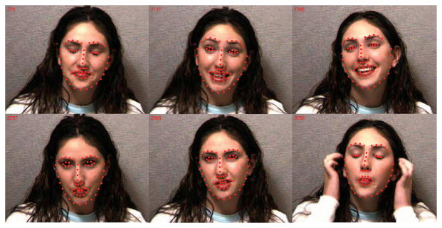
Over the last decade, appearance models have become increasingly important in computer vision and graphics. Parameterized Appearance Models (PAMs) (e.g., Active Appearance Models [37], [38], [39] and Morphable Models [40]) have been proven useful for detection, facial feature alignment, and face synthesis. In particular, AAMs have proven to be an excellent tool for aligning facial features with respect to a shape and appearance model. In our case, the AAM is composed of 66 landmarks that deform to fit perturbations in facial features. Person-specific models were trained on approximately five percent of the video [39]. Fig. 3 shows an example of AAM tracking of facial features in a single subject from the RU-FACS [18], [19] video data set.

Fig. 3.

AAM tracking across several frames.

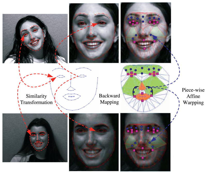
After tracking facial features using AAM, a similarity transform registers facial features with respect to an average face (see middle column in Fig. 4). In the experiments reported here, the face was normalized to 212 × 212 pixels. To extract appearance representations in areas that have not been explicitly tracked (e.g., nasolabial furrow), we use a backward piece-wise affine warp with Delaunay triangulation to set up the correspondence. Fig. 4 shows the two step process for registering the face to a canonical pose for AU detection. Purple squares represent tracked points and blue dots represent meaningful nontracked points. The dashed blue line shows the mapping between a point in the mean shape and its corresponding point in the original image. This two-step registration proves important toward detecting low intensity action units.

Fig. 4.

Two-step alignment.

3.2 Appearance Features

Appearance features for AU detection [11], [41] outperformed shape only features for some action units; see Lucey et al. [35], [42], [43] for a comparison. In this section, we explore the use of the SIFT [44] descriptors as appearance features.

Given feature points tracked with AAMs and SIFT descriptors are first computed around the points of interest. SIFT descriptors are computed from the gradient vector for each pixel in the neighborhood to build a normalized histogram of gradient directions. For each pixel within a subregion, SIFT descriptors add the pixel’s gradient vector to a histogram of gradient directions by quantizing each orientation to one of eight directions and weighting the contribution of each vector by its magnitude.

4 Dynamic Cascades with Bidirectional Bootstrapping

This section explores the use of a dynamic boosting techniques to select the positive and negative samples that improve detection performance in AU detection.

Bootstrapping [45] is a resampling method that is compatible with many learning algorithms. During the bootstrapping process, the active sets of negative examples are extended by examples that were misclassified by the current classifier. In this section, we propose Bidirectional Bootstrapping, a method to bootstrap both positive and negative samples.

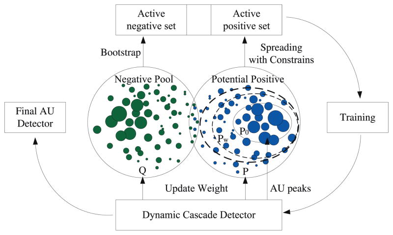
Bidirectional Bootstrapping begins by selecting as positive samples only the peak frames and uses Classification and Regression Tree (CART) [46] as a weak classifier (initial learning in Section 4.1). After this initial training step, Bidirectional Bootstrapping extends the positive samples from the peak frames to proximal frames and redefines new provisional positive and negative training sets (dynamic learning in Section 4.2). The positive set is extended by including samples that are classified correctly by the previous strong classifier (Cascade AdaBoost in our algorithm); the negative set is extended by examples misclassified by the same strong classifier, thus emphasizing negative samples close to the decision boundary. With the bootstrapping of positive samples, the generalization ability of the classifier is gradually enhanced. The active positive and negative sets then are used as an input to the CART that returns a hypothesis, which updates the weights in the manner of Gentle AdaBoost [47], and the training continues until the variation between previous and current Cascade AdaBoost become smaller than a defined threshold. Fig. 5 illustrates the process. In Fig. 5, P is a potential positive data set, Q is a negative data set (Negative Pool), P₀ is the positive set in the initial learning step, P_w is the active positive set in each iteration, the size of a solid circle illustrate the intensity of AU samples, the right ellipses illustrate the spreading of dynamic positive set. See details in Algorithms 1 and 2.

Fig. 5.

Bidirectional Bootstrapping.

4.1 Initial Training Step

This section explains the initial training step for DCBB. In the initial training step, we select the peaks and the two neighboring samples as positive samples, and a randomly selected sample of other AUs and non-AUs as negative samples. As in standard AdaBoost [14], we define the false positive target ratio (F_r), the maximum acceptable false positive ratio per cascade stage (f_r), and the minimum acceptable true positive ratio per cascade stage (d_r). The initial training step applies standard AdaBoost using CART [46] as a weak classifier as summarized in Algorithm 1.

Algorithm 1.

Initial learning

Input: Positive data set P0 (contains AU peak frames p and p ± 1); Negative data set Q (contains other AUs and nonAUs); Target false positive ratio Fr; Maximum acceptable false positive ratio per cascade stage fr; Minimum acceptable true positive ratio per cascade stage dr Initialize: Current cascade stage number t = 0; Current overall cascade classifier’s true positive ratio Dt = 1.0; Current overall cascade classifier’s false positive ratio Ft = 1.0; S0 = {P0, Q0} is the initial working set, Q0 ⊂ Q. The number of positive samples is Np. The number of negative samples is Nq = Np × R0, R0 = 8; While Ft > Fr t = t + 1; ft = 1.0; Normalize the weights ωt,i for each sample xi to guarantee that ωt = {ωt,i} is a distribution. While ft > fr For each feature ϕm, train a weak classifier on S0 and find the best feature ϕi (the one with the minimum classification error). Add the feature ϕi into the strong classifier Ht, update the weight in Gentle AdaBoost manner. Evaluate on S0 with the current strong classifier Ht, adjust the rejection threshold under the constraint that the true positive ratio does not drop below dr. Decrease threshold until dr is reached. Compute ft under this threshold. END While Ft+1 = Ft × ft; Dt+1 = Dt × dr; keep in Q0 the negative samples that the current strong classifier Ht misclassified (current false positive samples), record its size as Kfq. Use the detector Ht to bootstrap false positive samples from negative Q randomly and repeat until the negative working set has Nq samples. END While Output:  A t-levels cascade where each level has a strong boosted classifier with a set of rejection thresholds for each weak classifier.

4.2 Dynamic Learning

Once a cascade of peak frame detectors is learned in the initial learning stage (Section 4.1), we are able to enlarge the positive set to increase the discriminative performance of the whole classifier. The AU frames detector will become stronger as new AU positive samples are added for training. We added additional constraints to avoid adding ambiguous AU frames to the dynamic positive set. The algorithm is summarized in Algorithm 2.

Algorithm 2.

Dynamic learning

Input Cascade detector H0, from the Initial Learning step; Dynamic working set SD = {PD, QD}; All the frames in this action unit are represented as potential positive samples in the set P = {Ps, Pv}. Ps contains the strong positive samples, P0 contains peak related samples described above, P0 ∈ Ps. Pv contains ambiguous positive samples; A large negative data set Q contains all other AUs and nonAUs and its size is Na. Update positive working set by spreading within P and update negative working set by bootstrap in Q with the dynamic cascade learning process: Initialize: We set the value of Np as the size of P0. The size of the old positive data set is Np_old = 0 and the diffusion stage is t = 1. While (Np − Np_old)/Np > 0.1 AU Positive Spreading. Np_old = Np. Use the current detector on the data set P to potentially add more positive samples, Psp are all the positive samples that are determined by the cascade classifier Ht−1. Hard Constrain in Spreading. k Indexes the current AU event and i is the index to the current frame in this AU event. Calculate the similarity values (1) between the peak frame in event k and all peak frames with the lowest intensity value ‘A’, and denote the average similarity value with Sk. Calculate the similarity value between frame i and peak frame in event k, its value is Ski, if Ski < 0.5 × Sk, frame i will be excluded from Psp. After the above step, the remaining positive work set is Pw = Psp, Np = size of Psp. Using the Ht−1 detector to bootstrap false positive samples from the negative set Q until the negative working set Qw has Nq = β × R0 × Na samples, Na is different in AUs. Train the cascade classifier Ht with the dynamic working set {Pw, Qw}. As Rt varies, the maximum acceptable false positive ratio per cascade stage fmr also becomes smaller (2). t = t + 1; empty Pw and Qw. END While

The function to measure the similarity between the peak and other frames is the Radial Basis function between the appearance representation of two frames:

$$\begin{array}{l}{S}_k=\frac{1}{n}\sum _{j=1}^n\mathit{Sim}({\mathit{f}}_k,{\mathit{f}}_j),j\in [1:n],\\ S_{ik}=\mathit{Sim}({\mathit{f}}_i,{\mathit{f}}_k)=e^{-(\mathit{Dist}(i,k)/\mathit{max}(\mathit{Dist}(:,k))){,}^2}\\ \mathit{Dist}(i,k)={\left[\sum _{j=1}^m{(f_{kj}-f_{ij})}^2\right]}^{1/2},j\in [1:m].\end{array}$$ (1)

n refers to the total number of AU instances with intensity “A” and m is the length of the AU features.

The dynamic positive working set becomes larger, but the negative samples pool is finite, so f_mr needs to be changed dynamically. Moreover, N_q is function of N_a because different AU has different size of the negative samples pool. Some AUs (e.g., AU12) are likely to occur more often than others. Rather than tuning these thresholds one by one, we assume that the false positive ratio f_mr changes exponentially in each stage t, that is:

$$f_{m_r}=f_r\times (1-e^{-\alpha R_t}).$$ (2)

In our experimental setup, we set α as 0.2 and β as 0.04, respectively. We found empirically that those values are suitable for all the AUs to avoid lack of useful negative samples in RU-FACS database. After the spreading stage, the ratio between positive and negative samples becomes balanced, except for some rare AUs (e.g., AU4, AU10) where the unbalance is due to the scarceness of positive frames in the database.

5 Experiments

DCBB iteratively samples training frames and then uses Cascade AdaBoost for classification. To evaluate the efficacy of iteratively sampling training samples, Experiment 1 compared DCBB with the two standard approaches. They are selecting only peaks and alternatively selecting all frames between onsets and offsets. Experiment 1 thus evaluated whether iteratively sampling training images increased AU detection. Experiment 2 evaluated the efficacy of Cascade AdaBoost relative to SVM when iteratively sampling training samples. In our implementation, DCBB uses Cascade AdaBoost, but other classifiers might be used instead. Experiment 2 informs whether better results might be achieved using SVM. Experiment 3 explored the use of three appearance descriptions (Gabor, SIFT, and DAISY) in conjunction with DCBB (Cascade Adaboost as classifier).

5.1 Database

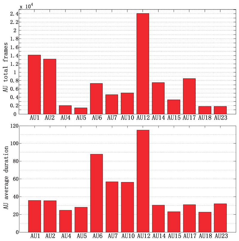
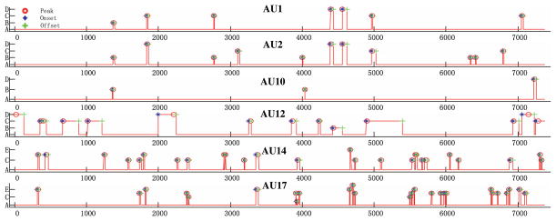
The three experiments all used the RU-FACS (a.k.a. M3) database [18], [19]. RU-FACS consists of video-recorded interviews of 34 men and women of varying ethnicity. Interviews were approximately two minutes in duration. Video from five subjects could not be processed for technical reasons (e.g., noisy video), which resulted in usable data from 29 participants. Metadata included manual FACS codes for AU onsets, peaks, and offsets. Because some AUs occurred too infrequently, we selected the 13 AUs that occur more than 20 times in the database (i.e., 20 or more peaks). These AUs are: AU1, AU2, AU4, AU5, AU6, AU7, AU10, AU12, AU14, AU15, AU17, AU18, and AU23. Fig. 6 shows the number of frames that each AU occurred and their average duration. Fig. 7 illustrates a representative time series for several AUs from subject S010. Blue asterisks represent onsets, red circles peak frames, and green plus signs the offset frames. In each experiment, we randomly selected 19 subjects for training and the other 10 subjects for testing.

Fig. 6.

(Top) Frame number from onset to offset for the 13 most frequent AUs in the M3 data set. (Bottom) The average duration of AU in frames.

Fig. 7.

AUs characteristics in subject S010, duration, intensity, onset, offset, and peak (frames as unit in X axis, Y axis is the intensity of AUs).

5.2 Experiment 1: Iteratively Sampling Training Images with DCBB

This experiment illustrates the effect of iteratively selecting positive and negative samples (i.e., frames) while training the Cascade AdaBoost. As a sample selection mechanism on top of the Cascade AdaBoost, DCBB could be applied to other classifiers as well. The experiment investigates whether the iteratively selecting training samples strategy is better than the strategy using only peak AU frames or the strategy using all the AU frames as positive samples. For different positive samples assignments, the negative samples are defined by the method used in Cascade AdaBoost.

We apply the DCBB method, described in Section 4 and use appearance features based on SIFT descriptors (Section 3). For all AUs, the SIFT descriptors are built using a square of 48 × 48 pixels for 20 feature points for the lower face AUs or 16 feature points for upper face (see Fig. 4). We trained 13 dynamic cascade classifiers, one for each AU, as described in Section 4.2, using a one versus all scheme for each AU.

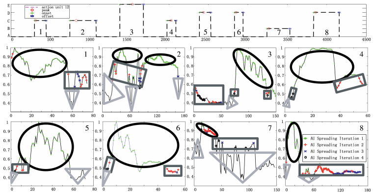
The top of Fig. 8 shows the manual labeling for AU12 of the subject S015. We can see eight instances of AU12 with varying intensities ranging from A (weak) to E (strong). The black curve in bottom figures represent the similarity (1) between the peak and the neighboring frames. The peak is the maximum of the curve. The positive samples in the first step are represented by green asterisks, in the second iteration by red crosses, in the third iteration by blue crosses, and in the final iteration by black circles. Observe that in the case of high-peak intensity, panels 3 and 8 (top right number in the similarity plots), the final selected positive samples contain areas of low similarity values. When AU intensity is low, panel 7, positive samples are selected if they have a high similarity with the peak, which reduces to the number of false positives. The ellipses and rectangles in the figures contain frames that are selected as positive samples, and correspond to strong and subtle AUs defined above. The triangles correspond to frames between the onset and offset that are not selected as positive samples, and represent ambiguous AUs in Fig. 1.

Fig. 8.

The spreading of positive samples during each dynamic training step for AU12. See text for the explanation of the graphics.

Table 1 shows the number of frames at each level of intensity and the percentage of each intensity that were selected as positive by DCBB in the training set. The letters “A–E” in left column refers to the level of AU intensities, The “Num” and “Pct” in the top rows refers to the number of AU frames at each level of intensity and the percentage of frames that were selected as positive examples at the last iteration of dynamic learning step, respectively. If there were no AU frames in one level of intensity, the “Pct” value will be “NaN.” From this table, we can see that DCBB emphasizes intensity levels “C,” “D,” and “E.”

TABLE 1.

Number of Frames at Each Level of Intensity and the Percentage of Each Intensity that Were Selected as Positive by DCBB

	AU1		AU2		AU4		AU5		AU6		AU7		AU10		AU12		AU14		AU15		AU17		AU18		AU23
	Num	Pct	Num	Pct	Num	Pct	Num	Pct	Num	Pct	Num	Pct	Num	Pct	Num	Pct	Num	Pct	Num	Pct	Num	Pct	Num	Pct	Num	Pct
A	986	46.3%	845	43.6%	325	37.1%	293	86.4%	119	40.2%	98	47.9%	367	61.3%	1561	38.1%	309	49.7%	402	72.6%	445	34.1%	134	87.4%	25	77.0%
B	3513	83.3%	3130	79.4%	912	70.4%	371	97.7%	1511	71.3%	705	93.4%	2131	90.8%	4293	73.3%	2240	93.9%	1053	89.7%	2553	70.1%	665	99.2%	190	87.8%
C	3645	90.9%	3241	91.3%	439	83.8%	110	99.7%	1851	87.8%	1388	97.9%	1066	92.8%	5432	82.0%	1040	95.6%	611	97.4%	1644	76.4%	240	98.7%	198	97.3%
D	2312	90.3%	1753	95.6%	73	79.6%	0	NaN	1128	84.2%	537	98.7%	572	88.6%	2234	83.5%	268	96.8%	68	98.6%	966	85.3%	83	98.6%	166	98.9%
E	151	99.3%	601	96.5%	0	NaN	23	96.6%	118	91.4%	153	98.5%	0	NaN	1323	92.4%	232	94.3%	0	NaN	226	80.2%	0	NaN	361	99.1%

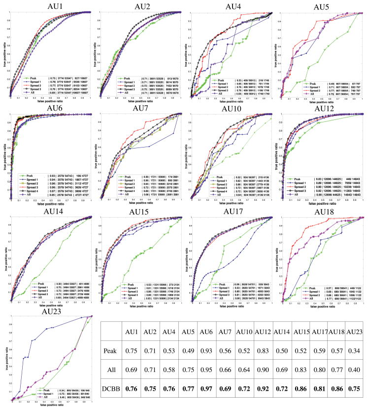
Fig. 9 shows the Receiver Operator Characteristic (ROC) curves for testing data (subjects not in the training) using DCBB. The ROC curves were obtained by plotting true positives ratios against false positives ratios for different decision threshold values of the classifier. Results are shown for each AU. In each figure, five or six ROC curves are shown: Initial learning corresponds to training on only the peaks (which is same as Cascade Adaboost without the DCBB strategy); spread x corresponds to running DCBB x times; All denotes using all frames between onset and offset. The first number between lines | in Fig. 9 denotes the area under the ROC; the second number is the size of positive samples in the testing data set; and separated by/is the number of negative samples in the testing data set. The third number denotes the size of positive samples in training working sets and separated by/the total frames of target AU in training data sets. AU5 has the minimum number of training examples and AU12 has the largest number of examples. We can observe that the area under the ROC for frame-by-frame detection improved gradually during each learning stage; performance improved faster for AU4, AU5, AU10, AU14, AU15, AU17, AU18, and AU23 than for AU1, AU2, AU6, and AU12 during Dynamic learning. Note that using all the frames between the onset and offset (“All”) typically degraded detection performance. The table below Fig. 9 shows the areas under the ROC when only the peak is selected for training, when all frames are selected and DCBB is used. DCBB outperformed both alternatives.

Fig. 9.

The ROCs improve with the spreading of positive samples: See text for the explanation of Peak, Spread x, and All.

Two parameters in the DCBB algorithms were manually tuned and remained the same in all experiments. One parameter specifies the minimum similarity value below which no positive sample will be selected. The threshold is based on the similarity (1). It was set at 0.5 after preliminary testing found results stable within a range of 0.2 to 0.6. The second parameter is the stopping criterion. We consider that the algorithm has converged when the number of new positive samples between iterations is less than 10 percent. In preliminary experiments, values less than 15 percent failed to change detection performance as indicated by ROC curves. Using the stopping criterion, the algorithm typically converged within three or four iterations.

5.3 Experiment 2: Comparing Cascade Adaboost and SVM When Used with Iteratively Sampled Training Frames

SVM and AdaBoost are two commonly used classifiers for AU detection. In this experiment, we compared AU detection by DCBB (Cascade AdaBoost as classifier) and SVM using shape and appearance features. We found that for both types of features (i.e., shape and appearance), DCBB achieved more accurate AU detection.

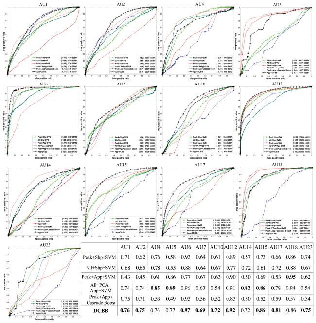
For compatibility with the previous experiment, data from the same 19 subjects as above were used for training and the other 10 for testing. Results are reported for the 13 most frequently observed AU. Other AU occurred too infrequently (i.e., fewer than 20 occurrences) to obtain reliable results and thus were omitted. Classifiers for each AU were trained using a one versus-all strategy. The ROC curves for the 13 AUs are shown in Fig. 10. For each AU, six curves are shown, one for each combination of training features and classifiers. “App + DCBB” refers to DCBB using appearance features; “Peak + Shp + SVM” refers to SVM using shape features trained on the peak frames (and two adjacent frames) [10]; “Peak + App + SVM” [10] refers to training an SVM using appearance features trained on the peak frame (and two adjacent frames); “All + Shp + SVM” refers to SVM using shape features trained on all frames between onset and offset; “All + PCA + App + SVM” refers to SVM using appearance features (after principal component analysis (PCA) processing) trained on all frames between onset and offset, here, in order to computationally scale in memory space, we reduced the dimensionality of the appearance features using PCA that preserves 98 percent of the energy. “Peak + App + Cascade Boost” refers to use the peak frame with appearance features and Cascade AdaBoost [14] classifier (will be equivalent to the first step in DCBB). As can be observed in the figure, DCBB outperformed SVM for all AUs (except AU18) using either shape or appearance when training in the peak (and two adjacent frames). When training the SVM with shape and using all samples, the DCBB performed better for 11 out of 13 AUs. In the SVM training, the negative samples were selected randomly (but the same negative samples when using either shape or appearance features). The ratio between positive and negative samples was fixed to 30. Compared with the Cascade AdaBoost (first step in DCBB that only uses the peak and two neighbor samples), DCBB improved the performance in all AUs.

Fig. 10.

ROC curve for 13 AUs using six different methods: AU peak frames with shape features and SVM(Peak + Shp + SVM); all frames between onset and offset with shape features and SVM (All + Shp + SVM); AU peak frames with appearance features and SVM (Peak + App + SVM); sampling one frame in every four frames between onset and offset with PCA to reduce appearance dimensionality and SVM (All + PCA + App + SVM); AU peak frames with appearance features and Cascade AdaBoost (Peak + App + Cascade Boost); DCBB with appearance features(DCBB).

Interestingly, the performance for AU4, AU5, AU14, and AU18 using the method “All + PCA + App + SVM” was better than “DCBB”. “All + PCA + App + SVM” uses appearance features and all samples between onset and offset. All parameters in SVM were selected using cross validation. It is interesting to observe that AU4, AU5, AU14, AU15, and AU18 are the AUs that have very few total training samples (only 1,749 total frames for AU4, 797 frames for AU5, 4,089 frames for AU14, 2,134 frames for AU15, 1,122 frames for AU18), and when having very little training data the classifier can benefit from using all samples. Moreover, the PCA step can help to remove noise. It is worth pointing out that best results were achieved by the classifiers using appearance SIFT instead of shape features, which suggests SIFT may be more robust to residual head pose variation in the normalized images. Using unoptimized MATLAB code, training DCBB typically required one to three hours depending on the AU and number of training samples.

5.4 Experiment 3: Appearance Descriptors for DCBB

Our findings and those of others suggest that appearance features are more robust than shape features in unposed video with small to moderate head motion. In the work described above, we used SIFT to represent appearance. In this section, we compare SIFT to two alternative appearance representations, DAISY and Gabor [24], [41].

Similar in spirit to the SIFT and DAISY descriptors are an efficient feature descriptor based on histograms. They have frequently been used to match stereo images [48]. DAISY descriptors use circular grids instead of the regular grids in SIFT; the former have been found to have better localization properties [49] and to outperform many state-of-the-art feature descriptors for sparse point matching [50]. At each pixel, DAISY builds a vector made of values from the convolved orientation maps located on concentric circles centered on the location. The amount of Gaussian smoothing is proportional to the radius of the circles.

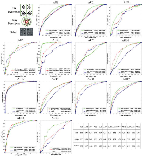
In the following experiment, we compare the performance on AU detection for three appearance representations, Gabor, SIFT, and DAISY using DCBB with Cascade Adaboost. Each was computed at the same locations (20 feature points in lower face, see Fig. 12). The same 19 subjects as before were used for training and 10 for testing. Fig. 11 shows the ROC detection curves for the lower AUs using Gabor filters at eight different orientations and five different scales, DAISY [50] and SIFT [44]. For most of AUs, ROC curves for SIFT, and DAISY were comparable. With respect to processing speed, DAISY was faster.

Fig. 12.

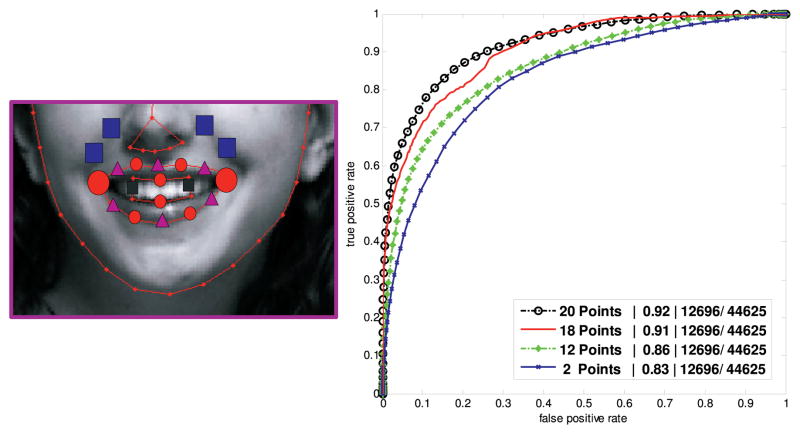
Using different numbers of feature points.

Fig. 11.

Comparison of ROC curves for 13 AUs using different appearance representations based on SIFT, DAISY, and Gabor representations.

An important parameter largely conditioning the performance of appearance-based descriptors is the number and location of features selected to build the representation. For computational considerations, it is impractical to build appearance representations in all possible regions of interest. To evaluate the influence of number of regions selected, we varied the number of regions, or points, in the mouth area from 2 to 20. As shown in Fig. 12, large red circles represent the location of two feature regions; adding blue squares and red circles increases the number to 12; adding purple triangles and small black squares increases the number to 18 and 20, respectively. Comparing results for 2, 12, 18, and 20 regions, or points, performance was consistent with intuition. While there were some exceptions, in general performance improved monotonically with the number of regions (Fig. 12).

6 Conclusions

An unexplored problem and critical to the success of automatic action unit detection is the selection of the positive and negative training samples. This paper proposes DCBB for this purpose. With few exceptions, DCBB achieved better detection performance than the standard approaches of selecting either peak frames or all frames between the onsets and offsets. We also compared three commonly used appearance features and the number of regions of interests or points to which they were applied. We found that the use of SIFT and DAISY improved accuracy relative to Gabor under same number of sampling points. For all three, increasing the number of regions or points monotonically improved performance. These findings suggest that DCBB when used with appearance features, especially SIFT or DAISY, can improve AU detection relative to standard selection methods for selecting training samples.

Several issues remain unsolved. The final Cascade Adaboost classifier has automatically selected the features and training samples that improve classification performance in the training data. During the iterative training, we have an intermediate set of classifiers (usually from three to five) that could potentially be used to model the dynamic pattern of AU events by measuring the amount of overlap in the resulting labels. Additionally, our sample selection strategy could be easily applied to other classifiers such as SVM or Gaussian Processes. Moreover, we plan to explore the use of these techniques in other computer vision problems such activity recognition, where the selection of the positive and negative samples might play an important role in the results.

Biographies

Yunfeng Zhu received the BSc degree in information engineering and the MSc degree in pattern recognition and intelligent system from the Xi’an Jiaotong University in 2003 and 2006, respectively. Currently, he is working toward the PhD degree in the Department of Electronic Engineering, Image and Graphics Institute, Tsinghua University, Beijing, China. In 2008 and 2009, he was a visiting student in the Robotics Institute at Carnegie Mellon University (CMU), Pittsburgh, Pennsylvania. His research interests include computer vision, machine learning, facial expression recognition, and 3D facial model reconstruction.

Fernando De la Torre received the BSc degree in telecommunications and the MSc and PhD degrees in electronic engineering from Enginyeria La Salle in Universitat Ramon Llull, Barcelona, Spain, in 1994, 1996, and 2002, respectively. In 1997 and 2000, he became an assistant and an associate professor, respectively, in the Department of Communications and Signal Theory at the Enginyeria La Salle. Since 2005, he has been a research faculty member in the Robotics Institute, Carnegie Mellon University (CMU), Pittsburgh, Pennsylvania. His research interests include machine learning, signal processing, and computer vision, with a focus on understanding human behavior from multimodal sensors. He directs the Human Sensing Lab (http://humansensing.cs.cmu.edu) and the Component Analysis Lab at CMU (http://ca.cs.cmu.edu). He coorganized the first workshop on component analysis methods for modeling, classification, and clustering problems in computer vision in conjunction with CVPR ’07, and the workshop on human sensing from video in conjunction with CVPR ’06. He has also given several tutorials at international conferences on the use and extensions of component analysis methods.

Jeffrey F. Cohn received the PhD degree in clinical psychology from the University of Massachusetts in Amherst. He is a professor of psychology and psychiatry at the University of Pittsburgh and an adjunct faculty member at the Robotics Institute, Carnegie Mellon University. For the past 20 years, he has conducted investigations in the theory and science of emotion, depression, and nonverbal communication. He has coded interdisciplinary and interinstitutional efforts to develop advanced methods of automated analysis of facial expression and prosody and applied these tools to research in human emotion and emotion disorders, communication, biomedicine, biometrics, and human-computer interaction. He has published more than 120 papers on these topics. His research has been supported by grants from the US National Institutes of Mental Health, the US National Institute of Child Health and Human Development, the US National Science Foundation (NSF), the US Naval Research Laboratory, and the US Defense Advanced Research Projects Agency (DARPA). He is a member of the IEEE and the IEEE Computer Society.

Yu-Jin Zhang received the PhD degree in applied science from the State University of Lige, Belgium, in 1989. From 1989 to 1993, he was a postdoctoral fellow and research fellow with the Department of Applied Physics and Department of Electrical Engineering at the Delft University of Technology, The Netherlands. In 1993, he joined the Department of Electronic Engineering at Tsinghua University, Beijing, China, where he has been a professor of image engineering since 1997. In 2003, he spent his sabbatical year as a visiting professor in the School of Electrical and Electronic Engineering at Nanyang Technological University (NTU), Singapore. His research interests include the area of image engineering that includes image processing, image analysis, and image understanding, as well as their applications. He has published more than 400 research papers and 20 books, including three edited english books: Advances in Image and Video Segmentation (2006), Semantic-Based Visual Information Retrieval (2007), and Advances in Face Image Analysis: Techniques and Technologies (2011). He is the vice president of the China Society of Image and Graphics and the director of academic committee of the Society. He is also a fellow of the SPIE. He is a senior member of the IEEE.

References

- 1.Ekman P, Friesen W. Facial Action Coding System: A Technique for the Measurement of Facial Movement. Consulting Psychologists Press; 1978. [Google Scholar]
- 2.Cohn JF, Ambadar Z, Ekman P. The Handbook of Emotion Elicitation and Assessment. Oxford Univ. Press; 2007. Observer-Based Measurement of Facial Expression with the Facial Action Coding System. [Google Scholar]
- 3.Cohn JF, Ekman P. Handbook of Nonverbal Behavior Research Methods in the Affective Sciences. Carnegie Mellon Univ; 2005. Measuring Facial Action by Manual Coding, Facial EMG, and Automatic Facial Image Analysis. [Google Scholar]
- 4.Ekman P, Rosenberg EL. What the Face Reveals: Basic and Applied Studies of Spontaneous Expression Using the Facial Action Coding System (FACS) Oxford Univ. Press; 2005. [Google Scholar]
- 5.Pantic M, Sebe N, Cohn JF, Huang T. Affective Multimodal Human-Computer Interaction. Proc 13th Ann ACM Int’l Conf Multimedia. 2005:669–676. [Google Scholar]
- 6.Zhao W, Chellappa R, editors. Face Processing: Advanced Modeling and Methods. Academic Press; 2006. [Google Scholar]
- 7.Li S, Jain A. Handbook of Face Recognition. Springer; 2005. [Google Scholar]
- 8.Tian Y, Cohn JF, Kanade T. Facial Expression Analysis. In: Li SZ, Jain AK, editors. Handbook of Face Recognition. Springer; 2005. [Google Scholar]
- 9.Tian Y, Kanade T, Cohn JF. Recognizing Action Units for Facial Expression Analysis. IEEE Trans Pattern Analysis and Machine Intelligence. 2001 Feb;23(2):97–115. doi: 10.1109/34.908962. [DOI] [PMC free article] [PubMed] [Google Scholar]
- 10.Lucey S, Ashraf AB, Cohn JF. Investigating Spontaneous Facial Action Recognition through AAM Representations of the Face. In: Delac K, Grgic M, editors. Face Recognition. InTECH Education and Publishing; 2007. pp. 275–286. [Google Scholar]
- 11.Bartlett MS, Littlewort G, Frank M, Lainscsek C, Fasel IR, Movellan JR. Recognizing Facial Expression: Machine Learning and Application to Spontaneous Behavior. Proc IEEE Conf Computer Vision and Pattern Recognition. 2005:568–573. [Google Scholar]
- 12.Valstar MF, Pantic M. Combined Support Vector Machines and Hidden Markov Models for Modeling Facial Action Temporal Dynamics. Proc IEEE Int’l Conf Computer Vision. 2007:118–127. [Google Scholar]
- 13.Tong Y, Liao WH, Ji Q. Facial Action Unit Recognition by Exploiting Their Dynamic and Semantic Relationships. IEEE Trans Pattern Analysis and Machine Intelligence. 2007 Oct;29(10):1683–1699. doi: 10.1109/TPAMI.2007.1094. [DOI] [PubMed] [Google Scholar]
- 14.Viola P, Jones M. Rapid Object Detection Using a Boosted Cascade of Simple Features. Proc IEEE Conf Computer Vision and Pattern Recognition. 2001:511–518. [Google Scholar]
- 15.Xiao R, Zhu H, Sun H, Tang X. Dynamic Cascades for Face Detection. Proc IEEE 11th Int’l Conf Computer Vision. 2007:1–8. [Google Scholar]
- 16.Yan SY, Shan SG, Chen XL, Gao W, Chen J. Matrix-Structural Learning (MSL) of Cascaded Classifier from Enormous Training Set. Proc IEEE Conf Computer Vision and Pattern Recognition. 2007:1–7. [Google Scholar]
- 17.Zhu YF, De la Torre F, Cohn JF. Dynamic Cascades with Bidirectional Bootstrapping for Spontaneous Facial Action Unit Detection. Proc. Workshops Affective Computing and Intelligent Interaction; Sept. 2009; [DOI] [PMC free article] [PubMed] [Google Scholar]
- 18.Frank MG, Bartlett MS, Movellan JR. The M3 Database of Spontaneous Emotion Expression. 2011. [Google Scholar]
- 19.Bartlett M, Littlewort G, Frank M, Lainscsek C, Fasel I, Movellan J. Automatic Recognition of Facial Actions in Spontaneous Expressions. J Multimedia. 2006;1(6):22–35. [Google Scholar]
- 20.Black MJ, Yacoob Y. Recognizing Facial Expressions in Image Sequences Using Local Parameterized Models of Image Motion. Int’l J Computer Vision. 1997;25(1):23–48. [Google Scholar]
- 21.De la Torre F, Yacoob Y, Davis L. A Probabilisitc Framework for Rigid and Non-Rigid Appearance Based Tracking and Recognition. Proc Seventh IEEE Int’l Conf Automatic Face and Gesture Recognition. 2000:491–498. [Google Scholar]
- 22.Chang Y, Hu C, Feris R, Turk M. Manifold Based Analysis of Facial Expression. Proc IEEE Conf Computer Vision and Pattern Recognition Workshop. 2004:81–89. [Google Scholar]
- 23.Lee C, Elgammal A. Facial Expression Analysis Using Nonlinear Decomposable Generative Models. Proc IEEE Int’l Workshop Analysis and Modeling of Faces and Gestures. 2005:17–31. [Google Scholar]
- 24.Bartlett M, Littlewort G, Fasel I, Chenu J, Movellan J. Fully Automatic Facial Action Recognition in Spontaneous Behavior. Proc Seventh IEEE Int’l Conf Automatic Face and Gesture Recognition. 2006:223–228. [Google Scholar]
- 25.Pantic M, Rothkrantz L. Facial Action Recognition for Facial Expression Analysis from Static Face Images. IEEE Trans Systems, Man, and Cybernetics. 2004 Jun;34(3):1449–1461. doi: 10.1109/tsmcb.2004.825931. [DOI] [PubMed] [Google Scholar]
- 26.Pantic M, Patras I. Dynamics of Facial Expression: Recognition of Facial Actions and Their Temporal Segments from Face Profile Image Sequences. IEEE Trans Systems, Man, and Cybernetics—Part B: Cybernetics. 2006 Apr;36(2):433–449. doi: 10.1109/tsmcb.2005.859075. [DOI] [PubMed] [Google Scholar]
- 27.Yang P, Liu Q, Cui X, Metaxas D. Facial Expression Recognition Using Encoded Dynamic Features. Proc. IEEE Conf. Computer Vision and Pattern Recognition; 2008. [Google Scholar]
- 28.Sun Y, Yin LJ. Facial Expression Recognition Based on 3D Dynamic Range Model Sequences. Proc 10th European Conf Computer Vision: Part II. 2008:58–71. [Google Scholar]
- 29.Braathen B, Bartlett M, Littlewort G, Movellan J. First Steps towards Automatic Recognition of Spontaneous Facial Action Units. Proc. ACM Workshop Perceptive User Interfaces; 2001. [Google Scholar]
- 30.Lucey P, Cohn JF, Lucey S, Sridharan S, Prkachin KM. Automatically Detecting Action Units from Faces of Pain: Comparing Shape and Appearance Features. Proc IEEE Conf Computer Vision and Pattern Recognition Workshops. 2009:12–18. [Google Scholar]
- 31.Cohn JF, Kanade T. Automated Facial Image Analysis for Measurement of Emotion Expression. In: Coan JA, Allen JB, editors. The Handbook of Emotion Elicitation and Assessment. 2006. pp. 222–238. Oxford Univ. Press Series in Affective Science. [Google Scholar]
- 32.Cohn JF, Sayette MA. Spontaneous Facial Expression in a Small Group Can Be Automatically Measured: An Initial Demonstration. Behavior Research Methods. 2010;42(4):1079–1086. doi: 10.3758/BRM.42.4.1079. [DOI] [PMC free article] [PubMed] [Google Scholar]
- 33.Valstar MF, Patras I, Pantic M. Facial Action Unit Detection Using Probabilistic Actively Learned Support Vector Machines on Tracked Facial Point Data. Proc IEEE Conf Computer Vision and Pattern Recognition Workshops. 2005:76–83. [Google Scholar]
- 34.Valstar M, Pantic M. Fully Automatic Facial Action Unit Detection and Temporal Analysis. Proc IEEE Conf Computer Vision and Pattern Recognition. 2006:149–157. [Google Scholar]
- 35.Lucey S, Matthews I, Hu C, Ambadar Z, De la Torre F, Cohn JF. Aam Derived Face Representations for Robust Facial Action Recognition. Proc Seventh IEEE Int’l Conf Automatic Face and Gesture Recognition. 2006:155–160. [Google Scholar]
- 36.Zeng Z, Pantic M, Roisman GI, Huang TS. A Survey of Affect Recognition Methods: Audio, Visual, and Spontaneous Expressions. IEEE Trans Pattern Analysis and Machine Intelligence. 2009 Jan;31(1):39–58. doi: 10.1109/TPAMI.2008.52. [DOI] [PubMed] [Google Scholar]
- 37.Cootes TF, Edwards G, Taylor C. Active Appearance Models. Proc European Conf Computer Vision. 1998:484–498. [Google Scholar]
- 38.De la Torre F, Nguyen M. Parameterized Kernel Principal Component Analysis: Theory and Applications to Supervised and Unsupervised Image Alignment. Proc IEEE Conf Computer Vision and Pattern Recognition. 2008 [Google Scholar]
- 39.Matthews I, Baker S. Active Appearance Models Revisited. Int’l J Computer Vision. 2004;60:135–164. [Google Scholar]
- 40.Blanz V, Vetter T. A Morphable Model for the Synthesis of 3D Faces. Proc ACM SIGGRAPH. 1999 [Google Scholar]
- 41.Tian YL, Kanade T, Cohn JF. Evaluation of Gabor-Wavelet-Based Facial Action Unit Recognition in Image Sequences of Increasing Complexity. Proc Seventh IEEE Int’l Conf Automatic Face and Gesture Recognition. 2002:229–234. [Google Scholar]
- 42.Ashraf AB, Lucey S, Chen T, Prkachin K, Solomon P, Ambadar Z, Cohn JF. The Painful Face: Pain Expression Recognition Using Active Appearance Models. Proc ACM Int’l Conf Multimodal Interfaces. 2007:9–14. doi: 10.1016/j.imavis.2009.05.007. [DOI] [PMC free article] [PubMed] [Google Scholar]
- 43.Lucey P, Cohn JF, Lucey S, Sridharan S, Prkachin KM. Automatically Detecting Pain Using Facial Actions. Proc Int’l Conf Affective Computing and Intelligent Interaction. 2009 doi: 10.1109/ACII.2009.5349321. [DOI] [PMC free article] [PubMed] [Google Scholar]
- 44.Lowe D. Object Recognition from Local Scale-Invariant Features. Proc IEEE Int’l Conf Computer Vision. 1999:1150–1157. [Google Scholar]
- 45.Sung K, Poggio T. Example-Based Learning for View-Based Human Face Detection. IEEE Trans Pattern Analysis and Machine Intelligence. 1998 Jan;20(1):39–51. [Google Scholar]
- 46.Breiman L. Classification and Regression Trees. Chapman and Hall; 1998. [Google Scholar]
- 47.Schapire R, Freund Y. Experiments with a New Boosting Algorithm. Proc 13th Int’l Conf Machine Learning. 1996:148–156. [Google Scholar]
- 48.Tola E, Lepetit V, Fua P. A Fast Local Descriptor for Dense Matching. Proc IEEE Conf Computer Vision and Pattern Recognition. 2008 [Google Scholar]
- 49.Mikolajczyk K, Schmid C. A Performance Evaluation of Local Descriptors. IEEE Trans Pattern Analysis and Machine Intelligence. 2005 Oct;27(10):1615–1630. doi: 10.1109/TPAMI.2005.188. [DOI] [PubMed] [Google Scholar]
- 50.Fua P, Lepetit V, Tola E. Daisy: An Efficient Dense Descriptor Applied to Wide Baseline Stereo. IEEE Trans Pattern Analysis and Machine Intelligence. 2010 May;32(5):815–830. doi: 10.1109/TPAMI.2009.77. [DOI] [PubMed] [Google Scholar]