Deep neural network with weight sparsity control and pre-training extracts hierarchical features and enhances classification performance: Evidence from whole-brain resting-state functional connectivity patterns of schizophrenia

Abstract

Functional connectivity (FC) patterns obtained from resting-state functional magnetic resonance imaging data are commonly employed to study neuropsychiatric conditions by using pattern classifiers such as the support vector machine (SVM). Meanwhile, a deep neural network (DNN) with multiple hidden layers has shown its ability to systematically extract lower-to-higher level information of image and speech data from lower-to-higher hidden layers, markedly enhancing classification accuracy. The objective of this study was to adopt the DNN for whole-brain resting-state FC pattern classification of schizophrenia (SZ) patients vs. healthy controls (HCs) and identification of aberrant FC patterns associated with SZ. We hypothesized that the lower-to-higher level features learned via the DNN would significantly enhance the classification accuracy, and proposed an adaptive learning algorithm to explicitly control the weight sparsity in each hidden layer via L₁-norm regularization. Furthermore, the weights were initialized via stacked autoencoder based pre-training to further improve the classification performance. Classification accuracy was systematically evaluated as a function of (1) the number of hidden layers/nodes, (2) the use of L₁-norm regularization, (3) the use of the pre-training, (4) the use of framewise displacement (FD) removal, and (5) the use of anatomical/functional parcellation. Using FC patterns from anatomically parcellated regions without FD removal, an error rate of 14.2% was achieved by employing three hidden layers and 50 hidden nodes with both L₁-norm regularization and pre-training, which was substantially lower than the error rate from the SVM (22.3%). Moreover, the trained DNN weights (i.e., the learned features) were found to represent the hierarchical organization of aberrant FC patterns in SZ compared with HC. Specifically, pairs of nodes extracted from the lower hidden layer represented sparse FC patterns implicated in SZ, which was quantified by using kurtosis/modularity measures and features from the higher hidden layer showed holistic/global FC patterns differentiating SZ from HC. Our proposed schemes and reported findings attained by using the DNN classifier and whole-brain FC data suggest that such approaches show improved ability to learn hidden patterns in brain imaging data, which may be useful for developing diagnostic tools for SZ and other neuropsychiatric disorders and identifying associated aberrant FC patterns.

Introduction

Resting-state functional MRI (rsfMRI) without a task paradigm has been successfully employed to exploit neuronal underpinnings implicated in neuropsychiatric disorders (Anand et al., 2005; Castellanos et al., 2008; Li et al., 2002), including schizophrenia (SZ) (Greicius, 2008; Jafri et al., 2008; Liang et al., 2006; Liu et al., 2008; Mingoia et al., 2012; Yu et al., 2012; Zhou et al., 2007). For example, Liu and colleagues (2008) presented evidence of significantly altered functional connectivity (FC) pairs (i.e., locally connected networks), or disrupted “small-world FC networks,” in the prefrontal, parietal, and temporal areas of the brain in patients with SZ. In that study, the hypothesis on dysfunctional network integration in SZ was supported by the lower strength of the FC in the pairs of nodes and decreased synchronization of functionally connected brain regions as well as the longer absolute path to reach global functional networks (Bullmore et al., 1997; Bullmore et al., 1998; Calhoun et al., 2009; Friston and Frith, 1995; Liu et al., 2008). In addition, Liang et al. (2006) reported that aberrant SZ-associated FC patterns were widely distributed throughout the entire brain (i.e., the FC levels of approximately 89% of the observed pairs of nodes were decreased), as opposed to showing a restricted pattern within only a few specific brain regions.

Machine-learning algorithms have been successfully deployed in the automated classification of altered FC patterns related to SZ (Arbabshirani et al., 2013; Du et al., 2012; Shen et al., 2010; Tang et al., 2012; Watanabe et al., 2014). In this regard, Du and colleagues (2012) developed a method combining kernel principal component analysis (PCA) and group independent component analysis (ICA) aimed at the computer-aided diagnosis of SZ, achieving 98% accuracy by using fMRI data acquired from an auditory oddball task paradigm. In addition, Shen et al. (2010) introduced an unsupervised learning-based classifier to discriminate SZ patients from HC subjects by applying a combination of nonlinear dimensionality reduction and self-organized clustering algorithms to rsfMRI data. The results of this analysis demonstrated the highest discriminating power for FC patterns between the cerebellum and the frontal cortex, with a classification accuracy of 92.3%. In addition, the altered resting-state functional network connectivity (FNC) among auditory, frontal-parietal, default-mode, visual, and motor networks were gainfully adopted for classification of SZ patients and 96% accuracy was achieved using k-nearest neighbors classifier (Arbabshirani et al., 2013). A recent schizophrenia classification challenge demonstrated clearly, across a broad range of classification approaches, the value of rsfMRI data in capturing useful information about this disease (Silva et al., 2014).

Of late, a strategy applying sparsity constraint to spatial patterns has favorably been deployed in various scenarios of fMRI data analysis directed toward extracting information from whole-brain FC patterns (Grosenick et al., 2013; Kim et al., 2012; Lee et al., 2008b; Watanabe et al., 2014). This explicit control of sparsity to analyze fMRI data also includes certain widely used ICA algorithms, such as the popular default algorithms of Infomax and FastICA, which jointly maximize sparsity and independence (Calhoun et al., 2013). This sparsity control has also been beneficial for brain decoding via fMRI data classification (Ng and Abugharbieh, 2011). The sparsity constraint strategy is particularly well-suited to fMRI data given the inherent high dimensionality and intra-subject variability. Moreover, sparsity constraint using total variation penalization (Michel et al., 2012) or anatomically-informed spatiotemporally smooth sparse constraint (Ng et al., 2012) for decoding of fMRI data can explicitly model intra/inter-subject variability, thus resulting in superior performance compared with the least absolute shrinkage and selection operator (LASSO)-based classifier (Michel et al., 2012; Ng and Abugharbieh, 2011; Ng et al., 2012).

The sparsity constraint strategy was recently put into play with rsfMRI data acquired from SZ patients and other neuropsychiatric patients, facilitating the identification of aberrant FC-based attributes, the extraction of distinct and sparse SZ-associated FC networks, and the subsequent application of these attributes and networks to automated classification and diagnosis (Cao et al., 2014; Watanabe et al., 2014). For instance, Watanabe et al. (2014) discovered clinically informative feature sets by using the same data set employed in the current study (see Methods section) via a sparsity constraint with a fused LASSO scheme for the conventional support vector machine (SVM) classifier. Altered FC patterns were prominent in the fronto-parietal networks, the default-mode networks (DMNs), and the cerebellar areas, and the corresponding accuracy was 71.9% (Watanabe et al., 2014).

A deep neural network (DNN) with multiple hidden layers has achieved unprecedented classification performance relative to the SVM and other conventional models (e.g., the hidden Markov model) in various data sets such as image and speech data (Graves et al., 2013; Krizhevsky et al., 2012). This technical breakthrough was accomplished by overcoming the limitations of traditional multilayer neural networks that are based on standard back-propagation algorithms and prone to over-fitting to the training data (Schmidhuber, 2014). More specifically, the distinct characteristics of DNN training encompass (1) unsupervised layer-wise pre-training followed by fine-tuning (Bengio et al., 2007), and (2) stochastic corruption of the input pattern or weight parameters via random zeroing, for example, a denoising autoencoder (Hinton et al., 2012; Vincent et al., 2010). Despite accumulating evidence showing the superiority of the DNN, previous applications of DNN to neuroimaging data are limited to only a few studies (Brosch and Tam, 2013; Hjelm et al., 2014; Plis et al., 2014; Suk et al., 2013). Among the limited attempts to apply the DNN to neuroimaging data, the restricted Boltzmann machine as a building block for the DNN network model has demonstrated its improved capacity to extract spatial and temporal information of fMRI data compared with conventional matrix factorization schemes, such as ICA and PCA algorithms (Hjelm et al., 2014). In addition, Suk et al. (2013) investigated the DNN training strategy by employing a stacked autoencoder (SAE) to discriminate Alzheimer’s disease patients from mild cognitive impairment patients. This was done by using volumetric information derived from structural MRI data combined with cerebral glucose metabolism data obtained by positron emission tomography. More recently, Plis et al. (2014) provided a validation study of DNN applied to several types of neuroimaging data, providing evidence that DNN can learn important features such as disease severity (Plis et al., 2014).

Whole-brain FC patterns from fMRI data have not yet been utilized as input patterns to demonstrate the efficacy of the DNN for classification of SZ or other neuropsychiatric disorders. Therefore, the objective of the present investigation was to enhance the classification accuracy of SZ patients vs. HC subjects by using the DNN classifier and whole-brain FC patterns estimated from rsfMRI data. The DNN has been applied to various data sets, such as image and speech data as well as neuroimaging data, with less than 1,000 input dimensions (i.e., number of nodes in the input layer) (Graves et al., 2013; Krizhevsky et al., 2012). Compared with these data sets, a dimension of the whole-brain FC patterns can easily reach approximately 5,000 when the whole brain is divided into 100 sub-regions. This high dimensionality would be confounded by a lack of straightforward interpretations of whole-brain FC patterns compared with those of speech, image data, and other neuroimaging modalities such as raw fMRI volumes and structural MRI data. Thus, training the DNN using complex and high-dimensional whole-brain FC patterns is inherently challenging. To this end, we evaluated our supposition that classification accuracy can be enhanced by (1) deploying sparsity control of DNN weight parameters and (2) systematically initializing the weight parameters via a pre-training scheme.

We defined a sparsity level of DNN weights as the ratio between a number of non-zero values of DNN weights and a total number of DNN weights (i.e., non-zero ratio). Then, to explicitly control the sparsity of the DNN weights, we developed an adaptive scheme to control the non-zero ratios of the weights between two connected layers to target levels. We then hypothesized that the DNN using the proposed scheme would improve the classification accuracy of SZ patients and HC subjects relative to the DNN without the proposed scheme as well as conventional approaches such as the SVM classifier. This is because hierarchical feature representations (i.e., a transition from lower-to-higher level information) of whole-brain FC patterns derived from rsfMRI data can be obtained from DNN weights with sparsity control and pre-training. Such hierarchical feature representations would not be similarly available from the DNN without the weight sparsity control and pre-training. In addition to evaluation of the classification performance, we assessed the validity of the learned lower-to-higher level features of the DNN classifier by using kurtosis and graph-theoretical modularity measures, as well as spatial correlation coefficients (CCs) between the learned features and the input FC patterns.

Materials and Methods

Overview

Figure 1 presents an overall flow diagram of the analysis. First, the raw fMRI data were preprocessed, and the whole-brain FC patterns were calculated by using Pearson’s CCs (Fig. 1a). Second, the FC patterns were used as input patterns to a DNN classifier, and the DNN classifier was trained and parameters were optimized by using training and validation data from subjects split from the cross validation (CV) framework during the training phase (Fig. 1b). Finally, a classification of SZ patient or HC subject was performed for each individual in the test data during the test phase (Fig. 1b). In addition, the weights of the DNN classifier were interpreted via qualitative visual inspection and quantitative evaluation.

Figure 1.

Overall flow diagram of the functional connectivity (FC) analysis. (a) Raw functional magnetic resonance imaging (fMRI) data were preprocessed, and the input patterns (i.e., whole-brain FC patterns) were extracted. (b) The FC patterns were used as input for the deep neural network (DNN) classifier. In the nested cross-validation scheme, the DNN classifier was trained by using the training (three out of five folds) and validation (one fold) data for parameter optimization employing optional sparsity control of weights and stacked autoencoder (SAE)-based pre-training. The trained DNN classifier was used to estimate classification accuracy using the test data in the remaining fold. BOLD, blood-oxygenation-level-dependent; ROI, region-of-interest; TS, time series; AAL, automated anatomical labeling; HC, healthy control; SZ, schizophrenia, N^HC, number of subjects in the HC group; N^SZ, number of subjects in the SZ group; ${\rho }_{\mathit{opt}}^{(J+1,J)}$, optimal target non-zero ratio of weights between the J^th and (J+1)^th hidden layers of the DNN obtained from the inner loop of nested cross validation using the training and validation data.

Data description

The rsfMRI data from SZ patients and HC subjects were obtained from the Neuroimaging Informatics Tools and Resources Clearinghouse (NITRC) website, contributed by the Centers of Biomedical Research Excellence (COBRE; fcon_1000.projects.nitrc.org/indi/retro/cobre.html) and also available on the collaborative informatics and neuroimaging suite (COINS) data exchange (coins.mrn.org/dx) (Calhoun et al., 2011; Scott et al., 2011). A diagnosis of SZ was made by using the Structured Clinical Interview for DSM Disorders (SCID; Diagnostic and Statistical Manual of Mental Disorders, DSM-IV) (First et al., 2012). Exclusion criteria comprised any history of neurological disorders, a history of mental retardation, a history of severe head trauma with a > 5 min loss of consciousness, and/or a history of substance abuse/dependence within the last 12 months. All participants completed a battery of neuropsychological tests, including the Wechsler Test of Adult Reading and the Wechsler Abbreviated Scale of Intelligence (Venegas and Clark, 2011; Wechsler, 1999). The SZ patients were also rated according to the Positive and Negative Syndrome Scale (PANSS) as a severity measure of their SZ symptoms (Kay et al., 1987). The SZ patients (n=72; with the exception of one subject) were all receiving various antipsychotic medications at the time of the study, corresponding to both traditional agents (e.g., haloperidol and perphenazine) and newly developed agents (e.g., olanzapine and risperidone).

A 3-Tesla Siemens Tim Trio scanner with a 12-channel head coil, and a single-shot full k-space echo-planar imaging (EPI) system and ramp sampling correction using the inter-commissural line as a reference were employed to acquire rsfMRI data while their eyes open, where time-of-echo (TE) = 29 ms, time-of-repetition (TR) = 2000 ms, voxel size = 3 × 3 × 4 mm³, in-plane voxel = 64 × 64, 33 slices, and number of volumes = 150. The first five volumes were removed to allow equilibration of the T₁-related signal. The remaining EPI volumes were preprocessed using statistical parametric mapping (SPM) software (SPM8; www.fil.ion.ucl.ac.uk/spm) in the order of slice-timing correction, realignment, and spatial normalization to the Montreal Neurological Institute (MNI) template with 3 mm isotropic voxel size, followed by spatial smoothing using an 8 mm isotropic full-width at half-maximum Gaussian kernel. The automated anatomical labeling (AAL) template (Tzourio-Mazoyer et al., 2002) available in the MNI space was re-sliced from a 2 mm to 3 mm isotropic voxel size using SPM8. Thus, each of the 116 AAL regions was readily available in each voxel of the normalized EPI volumes. Additionally, abrupt movements were minimized by utilizing the ArtRepair software toolbox (Raiko et al., 2012) which implements a “volume scrubbing” (Power et al., 2012). Thus, potential adverse effects of head-motion artifacts were minimized during the classification test, as well as during the qualitative/quantitative evaluation of the learned features.

Subjects (n=147 before screening) were excluded from the study if (1) the average displacement due to head motion during fMRI scanning, as estimated from the realignment parameters, exceeded 0.45 mm (Power et al., 2012); (2) the diagnostic results from the DSM-IV criteria were unrelated to SZ (n=4 subjects, as exemplified by late-onset dementia of the Alzheimer’s type as classified by the DSM-IV); and (3) the data acquisition process was incomplete (n=1 subject). From the remaining subjects, equal numbers (n=50) of individuals were assigned to the SZ and HC groups via a pseudo-randomized pick. Table 1 summarizes the sociodemographic information, neuropsychological test results, and clinical characteristics for each of the two study groups.

Table 1.

Summary of sociodemographics, neuropsychological test, and clinical characteristics for each of the HC and SZ groups.

	HC (Mean ± SD, N = 50)	SZ (Mean ± SD, N = 50)	p-value
Demographics
Age (years)	35.50 ± 11.88	35.94 ± 13.59	0.86
Gender (male/%)	34/68%	43/86%
Handedness (right/%)	48/96%	42/84%
Ethnicity (Caucasian/%)*	23/46%	25/50%
Neuropsychological performance*
WTAR standard score	109.93 ± 12.73	103.04 ± 13.07	1×10−2
WASI verbal IQ	108.17 ± 9.02	100.74 ± 16.63	9×10−3
WASI performance IQ	113.86 ± 12.58	104.83 ± 16.18	3×10−3
Clinical characteristics
Age of onset (years)		20.94 ± 6.95
Illness duration (years)		15.00 ± 11.85
PANSS positive		14.36 ± 4.78
PANSS negative		15.00 ± 5.36
PANSS general		29.42 ± 8.55
PANSS total		58.78 ± 14.35
Olanzapine equivalent dose (mg)		11.00 ± 6.32

HC: healthy control; SZ: schizophrenia patients; SD: standard deviation; WTAR: Wechsler test of adult reading; WASI: Wechsler abbreviated scale of intelligence; IQ: intelligence quotient; PANSS: positive and negative syndrome scale.

^*missing values from some subjects were removed in calculating the mean and SD)

FC analysis

The average blood-oxygenation-level-dependent (BOLD) time series (TS) across the voxels in each of the 116 regions of the AAL atlas were linearly detrended and bandpass filtered at 0.004–0.08 Hz. The average TS from each white matter (WM) and cerebrospinal fluid (CSF) area was also extracted and used to exclude non-neuronal components in the BOLD TS. The WM and CSF areas were defined from the voxels with a probability of > 99^th percentile in the apriori maps available in the SPM8 software package (Kim et al., 2013; Kim and Lee, 2013). In addition, six motion parameters (three rotations and three translations) obtained from the realignment step were employed as nuisance variables. These non-neuronal confounding factors were regressed out from the average BOLD TS for each AAL region via the least-squares error minimization scheme (Chai et al., 2012; Kim et al., 2015a; Kim et al., 2015b; Song et al., 2011). The Pearson’s CCs were then calculated using the resulting BOLD signals from all possible pairs (n=6,670) of the 116 AAL regions, a triangular portion of the CC matrix (Fig. 1a). The CCs were Fisher’s r-to-z transformed (Rosner, 2010). The z-scored FC levels for each subject were normalized to yield a zero mean and unit variance via pseudo z-scoring. The pseudo z-scored FC levels across all 6,670 pairs (₁₁₆C₂) of the AAL regions were used as input patterns for the DNN classifier.

DNN training with sparsity control of weights

The DNN layers consisted of multiple hidden layers and a softmax layer as an output layer. The target values of the two output nodes in the softmax layer were assigned as [1, 0]^T and [0, 1]^T for the input pattern from the HC group and the SZ group, respectively. The cost function, J(W) of the DNN for the supervised fine-tuning step was defined using the mean squared error (MSE), L₁-norm, and L₂-norm terms as follows:

$$J(\mathbf{W})=\frac{1}{2}\sum _{n=1}^N{\Vert {\mathbf{y}}^{(L),\{n\}}(\mathbf{W})-{\mathbf{t}}^{\{n\}}\Vert }^2+\sum _{J=0}^L{\beta }^{(J+1,J)}(t)\Vert {\mathbf{W}}^{(J+1,J)}\Vert +\sum _{J=0}^L\frac{{\gamma }^{(J+1,J)}}{2}{\Vert {\mathbf{W}}^{(J+1,J)}\Vert }^2$$ (1)

where y^(L),{n}(W) is a vector with elements of the output values at the L^th layer for the subject n in the training set, t^{n} is the target output values of the subject n (i.e., class information; [1 0]^T for HC and [0 1]^T for SZ), β^(J+1,J)(t) and γ^(J+1,J) are the L₁-norm and L₂-norm regularization parameters, respectively, between the J^th and (J+1)^th layer, N is the total number of subjects in the training set, and (L+1) is the number of the layers, including the input layer (i.e., the 0^th layer) and the output layer (i.e., the L^th layer).

A learning algorithm of DNN weights was derived from a stochastic gradient descent scheme to this cost function (also termed the fine-tuning step) as follows:

$$\begin{array}{l}{\mathbf{W}}^{(J+1,J)}(t+1)={\mathbf{W}}^{(J+1,J)}(t)-\mathrm{\Delta }{\mathbf{W}}^{(J+1,J)}(t),\\ \mathrm{\Delta }{\mathbf{W}}^{(J+1,J)}(t)=\alpha (t)\left({\mathrm{\Delta }}_{\mathit{MSE}}{\mathbf{W}}^{(J+1,J)}(t)+{\beta }^{(J+1,J)}(t)\mathit{sign}\left({\mathbf{W}}^{(J+1,J)}(t)\right)+{\gamma }^{(J+1,J)}{\mathbf{W}}^{(J+1,J)}(t)\right),\end{array}$$ (2)

where Δ_MSE W^(J+1,J)(t) is the first-order derivative of the cost function with respect to the W^(J+1,J)(t) weight parameters, or the weights between the J^th and (J+1)^th layer, and was previously used in a standard back-propagation algorithm (Bishop, 1995); t is the epoch number (i.e., one epoch was defined as the DNN weight updates derived from using all of the training data); and α(t) is the learning rate at the t^th epoch. The learning rate α(t) was initially set to 0.002 (i.e., α(0)=0.002) and then gradually reduced after the first 250 epochs (Bengio, 2013; Darken and Moody, 1992). Note that β^(J+1,J)(t) was adaptively controlled to reach a target sparsity level of weights between the J^th and (J+1)^th layers, and γ^(J+1,J) was fixed to 10⁻⁵ to prevent over-fitting of weights (Moody et al., 1995). A total of 500 epochs were used, and the number of hidden nodes was set to 50 for each of the hidden layers. To accelerate the learning procedure, a previous weight update term (or momentum) was added to the current weight update term (Bishop, 1995) as follows:

$${\mathbf{W}}^{(J+1,J)}(t+1)={\mathbf{W}}^{(J+1,J)}(t)-\alpha (t)\left(\mathrm{\Delta }{\mathbf{W}}^{(J+1,J)}(t)+m\mathrm{\Delta }{\mathbf{W}}^{(J+1,J)}(t-1)\right),$$ (3)

where t is the epoch number, and the learning rate m of this momentum (a fraction of the previous weight update term) was fixed to 0.1. This momentum term of the weight update accelerates the gradient descent learning to find an optimal point when the gradient of the MSE consistently points to the same direction (Bishop, 1995). The classification results using the DNNs with one to five hidden layers were obtained to test whether more hidden layers lead to better classification performance or saturate/degrade at a certain number of the hidden layers. A semi-batch learning process with a batch size of ten input vectors from ten subjects was utilized. The DNN training algorithm implemented in the publicly available DNN software toolbox was used with the above parameters in the MATLAB environment (github.com/rasmusbergpalm/DeepLearnToolbox).

Proposed scheme for sparsity control of DNN weights

Training of DNN weights is inherently challenging due to multiple hidden layers. This complication can be aggravated when whole-brain rsfMRI FC patterns are employed as input patterns. To overcome this issue, an approach was undertaken to explicitly control the degree of sparsity of the weights, or the weight sparsity, for each of the hidden layers of the DNN. The L₁-norm regularization parameter β^(J+1,J)(t) was then adaptively changed to achieve the target sparsity level in terms of the ratio of non-zero weights (hence, the lower the ratio of the non-zero weights, the higher the level of the weight sparsity, and vice versa). This approach therefore permits the systematic evaluation of associations between (1) the degrees of weight sparsity in each of the hidden layers during the training phase, and (2) the consequent classification accuracies during the test phase. In our proposed approach, an L₁-norm regularization parameter, β^(J+1,J)(t), was adaptively changed in each epoch, as follows:

$${\beta }^{(J+1,J)}(t+1)={\beta }^{(J+1,J)}(t)-\mu \left({\rho }^{(J+1,J)}-\mathit{nzr}\left({\mathbf{W}}^{(J+1,J)}(t)\right)\right),$$ (4)

where μ is the learning rate, fixed to a value of 10⁻⁵; ρ^{(J+1, J)} is the target non-zero ratio of W^{(J+1, J)}; and nzr(·) is a function to account for the non-zero ratio of a vector/matrix. β^{(J+1, J)}(t) was initially set to 10⁻³ and was bounded to a minimum value of 0 and maximum value of 10⁻² during the update. Various target non-zero ratios (ρ^{(J+1, J)} = 0.3, 0.5, 0.7, or 1.0) were tested for each hidden layer to reflect the potentially different optimal sparsity level in each layer. The optimal non-zero ratios for each of the hidden layers were determined among all combinatorial sets of non-zero ratios across the hidden layers when the validation accuracy was maximal. In addition, the reproducibility of the optimal non-zero ratios across the permuted CV sets was evaluated using the intra-class correlation coefficient (ICC) implemented in the MATLAB code available from MATLAB Central (www.mathworks.com/matlabcentral; “ICC.m” by A. Salarian) (Koch, 1982). Classification accuracies were evaluated using the test sets for these non-zero ratios. Note that the weights between the last hidden layer and the softmax layer were trained by using only L₂-norm regularization to fully minimize the MSE-based cost function.

Pre-training of DNN weights for initialization

Pre-training of DNN weights as opposed to random initialization has proven its utility to circumvent a local minimum and thus enhances the classification performance (Hinton et al., 2006; Larochelle et al., 2009). Similarly, using whole-brain FC patterns as input sample, we evaluated whether the pre-training of DNN weights would also improve the classification performance. To this end, an autoencoder (AE) algorithm was applied to minimize the reconstruction error of the input sample in the reconstructed input layer (left of Fig. 2), the output of the first hidden layer was used as input to the second hidden layer in the SAE scheme (right of Fig. 2), and the multilayer networks consisted of SAE pre-trained layers (middle of Fig. 2). More specifically, the weights, W^(1,0),e, and the bias, b^(0),e, for encoding the input sample were trained from the AE between the input layer (i.e., layer 0) and the first hidden layer (i.e., layer 1) to minimize a cost function defined from a MSE between the input and the reconstructed input sample. The weights, W^(2,1),e, and the bias, b^(1),e, were trained from the AE between the first hidden layer and the second hidden layer, whereby the output of the first hidden layer was used as the input to this AE. Then, the trained weights and bias terms from these AEs were stacked and used as initial weights of the DNN in the subsequent fine-tuning phase using the target output and actual output of the input sample. A random zeroing scheme was adopted for the AE, in which randomly selected elements (approximately 30% of the input pattern) were set to zero (Vincent et al., 2010). The learning rate α(t) in Eq. (2) was initially set to 0.01 and then gradually reduced after 500 epochs (Bengio, 2013). The total number of epochs was set to 1,000 to allow for convergence of the weights. The learning rate of the momentum factor was fixed to 0.1. The L₂-norm regularization parameter γ in Eq. (2) was set to 10⁻⁵ as in the fine-tuning step. In the DNN without pre-training and with sparsity control, the L₁-norm regularization parameter was also adaptively changed using Eq. (4). In a condition without pre-training, uniformly distributed random numbers within the range of $\pm 4\sqrt{6/\left(n_{in}+n_{\mathit{out}}\right)}$ were assigned as initial weights for random initialization, where n_in and n_out corresponded to the numbers of nodes in the input and output layers (Bengio, 2013). Table 2 summarizes four combinatorial scenarios for the training of DNN weights, depending on the use of sparsity control and/or pre-training. To evaluate the efficacy of the pre-training scheme in the DNN, the average learning curves of error rates across all permuted training/validation/test sets with the pre-training scheme were compared with the learning curves obtained without pre-training in the sparsity control-based L₁-norm regularization framework. The learning curves of the average non-zero ratio and adjusted L₁-norm regularization parameter during the training phase were also compared across the two weight initialization schemes.

Figure 2.

Pre-training-based initialization of deep neural network (DNN) weights. Left: The autoencoder (AE) architecture for the layer-wise pre-training; Right: the stacked AE (SAE) architecture between the input and the second hidden layers using the output of the first hidden layer as an input to the AE; Middle: SAE pre-training-based multilayer networks. SAE-based pre-training is performed using the weights and bias terms trained from the AE of each layer (please refer to the detailed description in the Methods section).

Table 2.

Pseudo codes of the DNN training depending on the use of (a) L₁-norm regularization for weight sparsity control and (b) SAE-based pre-training. The DNN training without L₁-norm regularization and without pre-training corresponds to a standard back-propagation algorithm.

		Initialization of weights
		With pre-training	Without Pre-training (i.e., random initialization)
Weight sparsity control	With L1-norm regularization	Pre-training of SAE with L1-norm regularization parameter as in Eq. (2) and (4) Fine-tuning with L1-norm regularization parameter as in Eq. (2) and (4)	Random initialization of weights Fine-tuning with L1-norm regularization parameter as in Eq. (2) and (4)
	Without L1-norm regularization (i.e. β(J+1,J)(t)= 0)	Pre-training of SAE without L1-norm regularization parameter Fine-tuning without L1-norm regularization parameter	Random initialization of the weights Fine-tuning without L1-norm regularization parameter

DNN, deep neural network; SAE, stacked autoencoder

Classification test

Classification performance was evaluated by using a nested CV framework during a training phase and the consequent test phase (Fig. 1b). In detail, a total of 50 subjects for each of the SZ and HC groups were split into five folds, with ten subjects in each fold for each group. During the training phase using the training data (three out of five folds) and the validation data (one fold), a grid search was conducted for several target non-zero ratios and optimal non-zero ratio parameters were obtained. Once the DNN classifier was trained, the classification performance was estimated by using the test data in the remaining fold. Using this scheme, a so-called “circular analysis” or “double dipping” issue could be prevented (Kriegeskorte et al., 2009). For instance, by using the DNN architecture with one hidden layer for each of the four target non-zero ratios, the DNN training and classification tests were both conducted 20 times, due to the numbers of scenarios required to select the training data (n=₅C₃) and the validation data (n=₂C₁). The classification tests were repeated ten times with a randomized split into five data folds, giving a total of 50 available error rates for each of the four target non-zero ratios. The reproducibility of these error rates for each of the conditions (i.e., with/without L₁-norm regularization and with/without pre-training) was evaluated using an ICC (Koch, 1982). Potentially significant main effects and/or interactions of these error rates were evaluated for all data via a three-way repeated measures analysis of variance (ANOVA). In the three-way ANOVA, one factor pertained to the use of sparsity control, one factor pertained to the use of pre-training, and one factor pertained to the number of hidden layers of the DNN. The resulting p-value was Bonferroni-corrected for multiple comparisons (i.e., d.f. = 999 due to 50 permuted training/validation/test data sets for each option of the sparsity-control/pre-training/five hidden layers).

SVM-based classification

For comparison with the DNN classifier, a SVM classifier with a linear kernel or a Gaussian radial basis function (RBF) kernel was used as implemented in the LIBSVM software package (www.csie.ntu.edu.tw/~cjlin/libsvm) (Chang and Lin, 2011). To train the SVM classifier, the soft margin parameter, C, and the γ_SVM parameter to control for RBF kernel size were optimized using the training data (three out of five folds) and the validation data (one fold) via a grid search (i.e., C = 2⁻⁵, 2⁻³, …, and 2¹⁵, and γ_SVM = 2⁻¹⁵, 2⁻¹³, …, and 2³) (Cristianini and Shawe-Taylor, 2000; Lee et al., 2009). The parameters of the SVM classifier were determined optimal when the validation accuracy was maximal, and the optimally chosen parameters across the CV sets were reported. Once the SVM classifier was trained, the classification performance was estimated using the test data in the remaining fold.

Learned features from the trained DNN and its qualitative interpretation via visualization

To test our hypothesis regarding the lower-to-higher level FC features of the DNN, the DNN weights were trained by taking into account the data from all of the subjects. This scheme avoids the complication of merging DNN weights obtained from various sets of training, validation, and test data, although classification accuracy is not simultaneously available. In this type of DNN training, the average non-zero ratio level (i.e., the weight sparsity) presenting the highest classification performance during the classification test is used to set the target non-zero ratio for each of the layers.

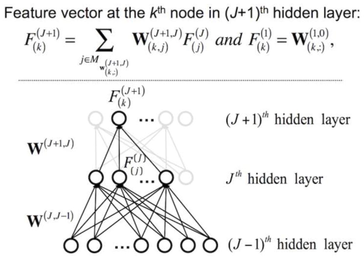
A linear combination of the weights across layers for feature representation from the trained DNN assumes that a hidden node can be characterized by the filters/weights of the previous layer that it is most strongly connected to (Lee et al., 2008a). For example, using the Mixed National Institute of Standards and Technology (MNIST) database of handwritten digits and natural images as inputs to the DNN, simple cell response (i.e., edge filters) in the early visual cortex was extracted from the weights between the input and first hidden layers, and the linear combination of these weights to the second layer resembled corner filters (Lee et al., 2008a). Similarly, the trained weights in each hidden layer of our DNN were visualized by linear projection from the input layer to the corresponding hidden layer (Fig. 3) (Denil et al., 2013; Lee et al., 2008a; Suk et al., 2014). Specifically, a feature vector at the k^th node in the (J+1)^th hidden layer was defined using the trained DNN weights as follows:

$$F_{(k)}^{(J+1)}=\sum _{j\in M_{{\mathbf{w}}_{(k,:)}^{(J+1,J)}}}{\mathbf{W}}_{(k,j)}^{(J+1,J)}{F}_{(j)}^J\mathit{and}{F}_{(k)}^{(1)}={\mathbf{W}}_{(k,:)}^{(1,0)},$$ (5)

where $M_{{\mathbf{w}}_{(k,:)}^{(J+1,J)}}$ is a set of the node indices at the J^th hidden layer that presents large magnitude values among the elements of the weight vector from the J^th hidden layer to the k^th node at the (J+1)^th hidden layer, ${\mathbf{W}}_{(k,:)}^{(J+1,J)}$. The choice of the number of hidden nodes for which weights were linearly combined might alter the characteristics of the DNN features; thus the DNN features were obtained for several numbers of linearly combined weights (i.e., 10, 15, and 30). Then, the reproducibility of the modularity and kurtosis values of the DNN features across these several numbers of the linear combination was evaluated via the ICC. The feature vectors were interpreted as the learned features of the whole-brain FC patterns in the corresponding hidden layer and then visualized using two options including (a) the BrainNet Viewer software (www.nitrc.org/projects/bnv) toolbox (Xia et al., 2013) and (b) the “circularGraph” toolbox available at MATLAB Central (www.mathworks.com/matlabcentral) to clearly illustrate the connectivity across the regions of interest (ROIs).

Figure 3.

Feature vector representation from the trained DNN weights. The learned feature vector, $F_{(k)}^{(J+1)}$, at the k^th hidden node in the (J+1)^th hidden layer is defined from a linear combination of the feature vectors in the J^th hidden layer (please refer to the detailed description in the Methods section). Input layer is defined as the 0^th layer.

Quantitative interpretation of learned features from trained DNN via spatial correlation and Fisher’s scores

Absolute values of spatial CCs between the learned features of the DNN and either the average FC patterns for the HC/SZ groups or the t-scored group-difference FC patterns (obtained from a two-sample t-test) were calculated. The capability of each hidden layer to discriminate between the two groups was also assessed using Fisher’s scores (Bishop, 1995), defined as follows:

$$F{S}_j^{(J)}=\frac{{\left(m_j^{(J),HC}-m_j^{(J),SZ}\right)}^2}{{\left({\sigma }_j^{(J),HC}\right)}^2-{\left({\sigma }_j^{(J),SZ}\right)}^2},$$ (6)

where the mean value of the j^th node input at the J^th hidden layer for the HC group $m_j^{(J),HC}=\frac{1}{N^{HC}}{\displaystyle \sum _{k=1}^{N^{HC}}}{h}_j^{(J),k}=\frac{1}{N^{HC}}{\displaystyle \sum _{k=1}^{N^{HC}}}{\displaystyle \sum _{i=1}^N}{\mathbf{W}}_{(j,i)}^{(J,J-1)}\mathit{sgm}\left(h_i^{(J-1),k}\right)$ ; sgm is the sigmoid function; the variance of the hidden node input for the HC group ${\sigma }_j^{(J),HC}=\frac{1}{N^{HC}}{\displaystyle \sum _{k=1}^{N^{HC}}}{\left(h_j^{(J),k}-m_j^{(J),HC}\right)}^2$; N is the number of hidden nodes; and N^HC and N^SZ are the number of subjects in the HC and SZ groups, respectively (a superscript indicates a layer index or a group label, and a subscript denotes a node index). The average Fisher’s score across 50 nodes in each hidden layer was taken as the score of the corresponding hidden layer. Hidden layers with higher Fisher’s scores represented layers with a greater capacity to discriminate between the two groups. To assess statistical significance of the hidden node input within each group and between the HC and SZ groups, a one-sample t-test and a two-sample t-test were administered using the hidden node input prior to application of sigmoid function of each hidden node.

The modularity of the learned features in each hidden layer was further analyzed via a graph-theoretical measurement (Girvan and Newman, 2002; Newman and Girvan, 2004) implemented in a graph-theoretical analysis toolbox (Hosseini et al., 2012). A modularity analysis incorporating the learned features of the DNN can reveal how whole-brain FC patterns are decomposed in each of the hidden layers to better discriminate SZ patients from HCs. The kurtosis values of the learned features in each layer were also calculated to evaluate the corresponding sparsity levels via non-Gaussianity and were compared between the layers using two-sample t-test.

Performance evaluation for several parameter sets

Our proposed continuous update of the L₁-norm regularization parameter β(t) based on the targeted non-zero ratio was compared with an approach that fixed the L₁-norm regularization parameter to one of several values (i.e., β = 10⁻², 10⁻³, and 10⁻⁴), in which the weight parameters were initialized with either pre-training or random initialization. The maximum number of epochs was set to 1,000 to train the DNN with the fixed L₁-norm regularization parameter because of the potentially slow convergence. The resulting learning curves of both the classification accuracy and non-zero ratios were collated across all of the permuted 5-fold CV sets. The L₂-norm regularization parameter γ was chosen from several additional values (i.e., 10⁻³, 10⁻⁴, and 10⁻⁶), and the classification performance was evaluated. The number of hidden layers and the number of nodes in each hidden layer can also be optimized using the training/validation data. Thus, we adopted a grid search to select the optimal number of hidden layers (i.e., among one to five hidden layers) and nodes (i.e., among 10, 25, 50, and 100) in each hidden layer.

Potential bias on classification performance due to head motion

The head motion of SZ patients is generally greater than that of HC subjects (Kong et al., 2014). Despite the volume scrubbing and removal of the motion-related component in the BOLD signal when the FC patterns were calculated in our present study, the classification performance could be positively biased due to head motions because the SZ patients potentially have less volume than the HC subjects. To evaluate this potential bias, the average framewise displacement (FD) for each subject was calculated, and averaged FD values for all subjects in the HC and SZ groups in the training sets were adopted as a regressor in the least-squares estimation. Then, the FC patterns with the confounding factor removed from the average FD values were calculated as follows and used as input samples for the DNN.

$$\begin{array}{l}\mathbf{Y}=\left[\begin{array}{cc}{\mathbf{x}}_{FD}& \mathbf{1}\end{array}\right]\left[\begin{array}{c}{\varphi }_{FD}\\ {\varphi }_{\mathit{bias}}\end{array}\right]+\epsilon =\mathbf{X}\mathrm{\Phi }+\epsilon ,\\ \widehat{\mathbf{Y}}=\mathbf{Y}-{\mathbf{x}}_{FD}{\varphi }_{FD}\end{array}$$ (7)

where Y and Ŷ (N×P; N is the number of subjects in the training set, and P is the number of elements [i.e., 6,670] in the FC pattern for each subject) are the FC patterns for all subjects in the HC and SZ groups in the training set with and without the FD components, respectively; x_FD (N×1) is the FD values for all subjects; 1 is a vector with an element of 1 to adjust a bias of the FC level; and ϕ_FD and ϕ_bias are the regression coefficients of the average FD values and the bias obtained from the least-squares estimation, respectively. The estimated coefficient of the FD (i.e., ϕ_FD) was used to remove the FD component of the FC patterns for the subjects in the test set. The FD-removed FC patterns were used as inputs of (1) the DNN classifier (with three hidden layers and 50 nodes in each hidden layer) by applying both the pre-training and weight sparsity control strategies and (2) the SVM classifiers with linear and RBF kernels. As a result, classification performance obtained from 50 randomly permuted training/validation/test data was reported along with the kurtosis and skewness values of the FC patterns with and without FD components.

Classification test employing FC patterns of functionally parcellated regions from group ICA

The average BOLD signal could potentially smooth out useful subtle patterns between BOLD signals. These hundreds or even thousands of BOLD signals could be very heterogeneous within each AAL region since the BOLD signal in each voxel may come from many different brain networks. To alleviate this potential limitation, an alternative method to functionally parcellate the brain networks was considered using a group ICA (GICA) (Calhoun and Adali, 2012; Calhoun et al., 2001). Subsequently, the time-courses (TCs) of the brain networks (i.e., spatial patterns) of independent components (ICs) were used to calculate FC patterns across these brain networks (Arbabshirani et al., 2013).

This functional parcellation was conducted in the CV framework. In detail, the preprocessed rsfMRI data from the training/validation sets (i.e., subjects) were analyzed using a spatial GICA as implemented in the GIFT toolbox (mialab.mrn.org/software/gift). Two-step dimension reduction was applied via a PCA, and the reduced dimensions in subject and group levels were 100 and 145, respectively. Then, 145 ICs were estimated from the Infomax algorithm (Bell and Sejnowski, 1995). Once the group spatial patterns (SPs) of the 145 ICs were estimated from GICA using the training/validation data to parcellate the whole brain into 145 regions, the SPs and TCs corresponding to the 145 brain regions were estimated using the spatio-temporal dual-regression applied to preprocessed rsfMRI data for each subject in the training/validation/test sets (Silva et al., 2014). The dual-regression estimates were (1) individual TCs using a group SPs as regressors and (2) individual SPs using the individual TCs as regressors (Beckmann and Smith, 2005; Calhoun and Adali, 2012; Du et al., 2012; Kim et al., 2012).

Each voxel was assigned to one of the SPs (i.e., brain regions) of 145 ICs if the t-score of the voxel (available from one-sample t-test using SPs across the training/validation data) of the assigned IC was greater than that of the remaining ICs. The probabilities that each voxel belongs to gray matter (GM), WM, and CSF are readily available in a priori maps of these three brain structures in SPM8. Thus, the proportions of the GM, WM, or CSF areas in each of the brain regions (i.e., SPs of ICs) were calculated by counting the number of voxels of the corresponding structure. Then, the top 116 ICs with greater proportions of GM than WM or CSF (i.e., 116 functionally parcellated brain regions) were selected to match the number of brain regions defined in the AAL template.

The TCs of these 116 ICs were used to calculate the FC patterns of the functionally parcellated brain regions. The six motion parameters (three rotations and three translations) obtained from the realignment step were regressed out from the TCs to remove any potential confounding factors due to head motion. Subsequently, the Pearson’s CC values were calculated and Fisher’s r-to-z transformed. An optimal non-zero ratio between two subsequent layers ρ^(J+1,J) was identified via a grid search from 0.3 to 1.0 with an interval of 0.1 (excluding 0.9) to include the grid search range of the non-zero ratios applied to the FC patterns using the AAL template. The classification test was performed using the DNNs with one to five hidden layers and with both pre-training and the proposed weight sparsity control schemes.

Results

Group-level FC patterns

The number of removed and interpolated volumes by volume scrubbing (mean ± the standard deviation, SD: 2.9 ± 3.5 and 5.7 ± 6.6 from the HC and SZ group, respectively) was not significantly different between the two groups (uncorrected p > 0.05) from the Mann-Whitney U test (Mann and Whitney, 1947). Figure 4 illustrates the average FC patterns for each group and the group differences between the HC and SZ groups obtained by using a two-sample t-test. The average FC patterns showed prominent intra-network patterns involving the frontal, visual, subcortical, and cerebellar areas, as well as inter-network patterns involving DMNs and the fronto-temporal, cortical-thalamus, cortical-cerebellar, and subcortical-cerebellar networks (Liu et al., 2008; Salvador et al., 2005). The FC patterns were statistically different (uncorrected p < 0.05) between the two groups in the fronto-temporal, cortical-thalamus, and cortical-cerebellar networks.

Figure 4.

Group-level functional connectivity (FC) patterns. (a) Average FC patterns in the healthy control (HC) and schizophrenia (SZ) groups and (b) group differences in the FC patterns (evaluated via a two-sample t-test with a threshold of uncorrected p-values of < 0.05) are shown. Positive t-scores indicate greater FC level from HC group than SZ group. SC, subcortical area; CB, cerebellum.

Classification performance depending on weight sparsity levels

Figure 5a exemplifies the learning curves of (1) the target non-zero ratio ρ^(J+1,J) (i.e., 0.5) of the DNN weights and (2) the L₁-norm regularization parameter, β^(J+1,J)(t), for the DNN with three hidden layers. The non-zero ratio was rapidly converged to the target value after several hundreds of epochs by adjusting β^(J+1,J)(t). Figure 5b shows the average learning curves of the DNNs with and without pre-training in the weight sparsity control framework. The faster convergence and the lower minimum error rate that were achieved from pre-training (i.e., 14.2%) compared with that from random initialization (i.e., 20.2%) may indicate that pre-training facilitates the initialization of DNN weights to render the optimization process of the initial weights more effectively as opposed to the random initialization (Erhan et al., 2010).

Figure 5.

(a) Learning curves are exemplified for (i) the non-zero ratio of weights between the input and first hidden layers controlled during the training phase (target value = 0.5), and (ii) the L₁-norm regularization parameter adaptation for the sparsity control of weights between the input and first hidden layers using the DNN with three hidden layers. (b) Averaged learning curves of error rates from the training, validation, and test data (top) and the learning curves of the non-zero ratio and L₁-norm regularization parameter (bottom). DNN, deep neural network.

Figure 6 depicts the average error rates obtained from 50 randomly permuted training/validation/test data for each of the target non-zero ratios and for the DNNs with several numbers of hidden layers. The average error rate of the DNN with one hidden layer (22.5%) was lowest when the target non-zero ratio was 0.5 (Fig. 6a). For the DNN with three hidden layers, the average error rate was 14.2% when the target non-zero ratios were 0.5, 0.7, and 0.7 from the first, second, and third hidden layers, respectively (Fig. 6c). Figure 6f shows the optimal (i.e., when the error rate was at its minimum) non-zero ratio for each of the hidden layers obtained via explicit control of the weight sparsity for each of the DNNs with several numbers of hidden layers. Overall, the optimal non-zero ratio of the first hidden layer was consistently smaller than that of the higher hidden layers (Bonferroni-corrected p < 10⁻⁶, one-way ANOVA). For example, the average non-zero ratios for the DNN with three hidden layers were 0.52 for the first hidden layer, 0.72 for the second hidden layer, and 0.85 for the third hidden layer. Figure 7 shows the line plots of the non-zero ratio parameters optimally chosen for the DNNs with several numbers of hidden layers. The ICC value for the DNN with three hidden layers was maximal (i.e., 0.82); thus the optimally determined non-zero ratios were most reproducible from the DNN with three hidden layers among those tested.

Figure 6.

Error rates for several target non-zero ratios. Error rates are shown for deep neural networks (DNNs) with (a) one hidden layer, (b) two hidden layers, (c) three hidden layers, (d) four hidden layers, and (e) five hidden layers. (f) The resulting non-zero ratios for each layer (mean ± SD) are presented for the DNNs with one, two, three, four, or five hidden layers. ρ^{(J+1, J)} is the target non-zero ratio of weights W^(J+1,J) between the J^th and (J+1)^th layer (e.g., the 0 layer is the input layer, and the 1^st layer is the first hidden layer). The optimal non-zero ratio in each layer is determined using the validation data after the DNN has been trained using the training data for all combinatorial sets of non-zero ratios across the layers. The error rates are obtained using the test data.

Figure 7.

The non-zero ratio parameters optimally chosen for each of the hidden layers from the DNN with one to five hidden layers. The optimal non-zero ratios were found when the validation accuracy was maximal among the sets of non-zero ratios across hidden layers. The line in each subplot indicates each of the randomly permuted CV sets with training/validation/test data. ICC, intra-class correlation coefficient; CV, cross validation.

Classification performance depending on pre-training

Figure 8 summarizes the error rates of the DNNs with several numbers of hidden layers and (a) sparsity control and SAE-based pre-training (DNNwSwP), (b) sparsity control but no pre-training (DNNwSwoP), (c) SAE-based pre-training but no sparsity control (DNNwoSwP), and (d) neither sparsity control nor pre-training (DNNwoSwoP). Overall, SAE-based pre-training further reduced the error rates of the DNN compared with random initialization. This trend was particularly evident for DNNs with more than two hidden layers. Average error rates (± the SD) from the DNN with sparsity control and SAE-based pre-training were 22.5 (± 0.7), 17.6 (± 0.4), 14.2 (± 0.4), 14.5 (± 1.2), and 16.6 (± 2.2)% for one, two, three, four, and five hidden layers, respectively. Furthermore, the average error rates (± the SD) from the DNN with sparsity control but no pre-training were 22.7 (± 1.0), 20.8 (± 0.9), 20.2 (± 1.2), 24.1 (± 1.4), and 25.2 (± 1.4)% for one, two, three, four, and five hidden layers, respectively. Error rates from the DNN with a standard back-propagation algorithm (i.e., without sparsity control or pre-training) were 25.1 (± 1.8), 23.1 (± 1.5), 25.1 (± 1.4), 25.0 (± 1.7), and 27.0 (± 2.1)%, respectively. The classification results from the five hidden layers were substantially degraded compared with the results from the three hidden layers with pre-training and sparsity control (Bonferroni-corrected p < 10⁻² from a paired t-test; d.f. = 98). Table 3 summarizes the error rates, sensitivities, and specificities for all combinatorial scenarios of the training strategies. The ICC values using the error rates across the pre-training and random initialization methods were greater from the DNN with three (0.49) and four (0.59) hidden layers (i.e., more reproducible) than from the DNNs with one (0.00), two (0.30), and five (0.29) hidden layers. When the pre-training initialization was used, the error rates from the DNN training with/without the L₁-norm regularization schemes were reproducible when the DNNs with two (0.48), three (0.32), and four (0.51) hidden layers were deployed rather than the DNNs with one (0.04) and five (0.15) hidden layers. A three-way repeated measures ANOVA revealed that the main effects of sparsity control, pre-training, and the number of hidden layers to the error rates were all statistically significant (Bonferroni-corrected p < 10⁻⁷; d.f. = 999). Moreover, significant interactions were observed between (1) the number of hidden layers and the use of the sparsity control (Bonferroni-corrected p < 0.05; d.f. = 499), and (2) the number of hidden layers and the use of the pre-training (Bonferroni-corrected p < 10⁻⁷; d.f. = 499).

Figure 8.

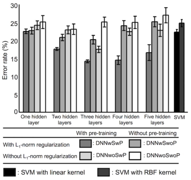
Comparison of error rates. Error rates are shown for deep neural networks (DNNs) with (a) L₁-norm regularization of weights (i.e., weight sparsity control) and stacked autoencoder (SAE)-based pre-training (DNNwSwP), (b) weight sparsity control but no pre-training (i.e., random initialization) (DNNwSwoP), (c) pre-training but no weight sparsity control (DNNwoSwP), and (d) neither weight sparsity control nor pre-training (DNNwoSwoP) for one, two, three, four, or five hidden layers, as well as for (e) the support vector machine (SVM) with a linear kernel or a Gaussian radial basis function (RBF) kernel. The DNN training neither weight sparsity control nor pre-training corresponds to a standard back-propagation algorithm.

Table 3.

Classification performance in terms of error rate (mean ± SD), sensitivity, and specificity. Sensitivity was defined as the ratio between (i) the number of true positives (i.e., correctly classified SZ patients) and (ii) the sum of the true positives and false negatives (i.e., incorrectly classified SZ patients). Specificity was defined as the ratio between (i) the number of true negatives (i.e., correctly classified HC subjects) and (ii) the sum of the true negatives and false positives (i.e., incorrectly classified HC subjects). The DNN training without L₁-norm regularization and without pre-training (i.e., random initialization) corresponds to a standard back-propagation algorithm. The ICC values were obtained using the error rates from the with/without pre-training approaches across all the permuted sets, or using the error rates from the with/without L₁-norm regularization schemes across all the permuted sets.

Number of hidden layer	Weight sparsity control	Initialization of weights		ICC
		With pre-training	Without Pre-training
		Error rate (Sensitivity; Specificity)	Error rate (Sensitivity; Specificity)
1	With L1-norm regularization	22.5 ± 0.7 (77.1; 77.9)	22.7 ± 1.2 (75.8; 78.8)	0.00
	Without L1-norm regularization	24.2 ± 1.2 (77.0; 74.6)	25.1 ± 1.8 (74.4; 75.4)	0.00
	ICC	0.04	0.03
2	With L1-norm regularization	17.6 ± 0.4 (82.6; 82.2)	20.8 ± 0.9 (79.9; 78.6)	0.30
	Without L1-norm regularization	22.9 ± 1.1 (76.8; 77.4)	23.1 ± 1.5 (77.1; 76.7)	0.00
	ICC	0.48	0.06
3	With L1-norm regularization	14.2 ± 0.4 (86.3; 85.3)	20.2 ± 1.2 (79.8; 79.8)	0.49
	Without L1-norm regularization	17.5 ± 0.9 (83.0; 82.0)	25.1 ± 1.4 (74.9; 74.9)	0.44
	ICC	0.32	0.22
4	With L1-norm regularization	14.5 ± 1.2 (85.3; 87.5)	24.1 ± 1.4 (75.4; 76.4)	0.59
	Without L1-norm regularization	22.4 ± 1.0 (77.0; 78.2)	25.0 ± 1.7 (75.1; 74.9)	0.05
	ICC	0.51	0.00
5	With L1-norm regularization	16.6 ± 2.2 (83.3; 83.5)	25.2 ± 1.4 (75.4; 74.2)	0.29
	Without L1-norm regularization	22.8 ± 1.7 (77.5; 76.9)	27.0 ± 2.1 (73.0; 74.9)	0.06
	ICC	0.15	0.00

ICC, intra-class correlation coefficient

Classification performance from SVM

Error rates for the SVM classifier with a linear kernel (22.3 ± 0.8%) or a RBF kernel (24.9 ± 1.0%) were generally inferior compared with error rates obtained for DNNs with sparsity control and pre-training (Fig. 8). Figure 9 illustrates that the optimal parameters of the SVM from the grid search were 2¹³ for the soft margin parameter C (using a linear kernel), 2⁹ for the soft margin parameter C, and 2⁻² for the RBF kernel size γ_SVM (using an RBF kernel).

Figure 9.

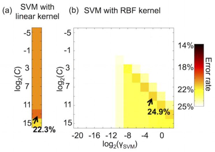
Optimally chosen SVM parameters: (a) the soft margin parameter C from the SVM with a linear kernel and (b) C and the RBF kernel size γ_SVM from the SVM with an RBF kernel.

Hierarchical features interpreted from DNN weights

The learned features of the first hidden layer of the DNN with three hidden layers are visualized in Figures 10a–c and Figure S1 (see Tables S1–S4 for details). These learned features represent (1) the reduced FC level from SZ group between the cerebellum and the subcortical areas, and (2) both the reduced and increased FC levels from SZ group between the thalamus and the cortical regions (the first column in Fig. 10c, Table S1) (Çetin et al., 2014). The posterior cingulate cortex (PCC), angular gyrus, paracentral lobule, and occipital gyrus showed aberrant FC patterns (the second column in Fig. 10c, Table S2). The frontal areas, temporal lobe, and occipital gyrus exhibited reduced FC level from SZ group (the third column in Fig. 10c, Table S3), in addition to altered striatal FC patterns (the fourth column in Fig. 10c, Table S4). The learned features of the second and the third hidden layer showed densely populated FC patterns across multiple brain regions (Figs. 10a–b). All of the learned features for each hidden node in each hidden layer are visualized in Figures S1–S3. Overall, lower-level/localized features from the first hidden layer (Fig. S1) and higher-level/global features from the second (Fig. S2) and third (Fig. S3) hidden layers were observed. The first and second hidden node input from the first hidden layer were statistically different between the HC and SZ groups (Fig. 10c; Bonferroni-corrected p < 10⁻⁴ from a two-sample t-test; d.f. = 99), whereas all four hidden node input from the third hidden layer were statistically different between the two groups (Fig. 10a; Bonferroni-corrected p < 10⁻¹⁴ from a two-sample t-test; d.f. = 99). Moreover, all four hidden node input from the third hidden layer was statistically different from zero within each group presenting opposite signs across the two groups (Fig. 10a; Bonferroni-corrected p < 10⁻⁵ from a one-sample t-test; d.f. = 49), and thus this indicates that the hidden node output with sigmoid node function is readily separable from 0.5.

Figure 10.

Learned features of the top four hidden nodes (sorted by Fisher’s scores) in the (a) third, (b) second, and (c) first hidden layers. In the learned features, all weight values above 0.2 or below −0.2 are shown. Each number in the circular graphs indicates the automated anatomical labeling (AAL) region (as defined in the AAL toolbox for SPM8; odd indices are shown for brevity). The boxplots represent the mean and standard deviation of the corresponding hidden node input values prior to application of the sigmoid node function. The number in each boxplot is the Fisher’s score of the corresponding hidden node input. The thickness of each red or blue line represents the normalized magnitude of the weight parameters (i.e., the thicker the line, the greater the magnitude). HC, healthy control; SZ, schizophrenia; CB, cerebellum; SC, subcortical region; PCG, postcentral gyrus; PCL, paracentral lobule; SOG, superior occipital gyrus; PCC, posterior cingulate cortex; MOG, middle occipital gyrus; IFG, inferior frontal gyrus; ITG, inferior temporal gyrus; a.u., arbitrary unit.

Figure 11a shows the increased average absolute values of the spatial CCs between the learned features and (1) the mean FC patterns from the SZ or HC group, as well as (2) the group differences in the FC patterns between the SZ and HC groups in the higher layer (see Fig. 4b). Meanwhile, Figure 11b shows the average Fisher’s score of each hidden layer for the DNN with three hidden layers. Note that the Fisher’s score of the third hidden layer was significantly larger than that of the first hidden layer (1.94 ± 0.30 and 0.07 ± 0.01 from the third and first hidden layers, respectively; Bonferroni-corrected p < 10⁻⁴ from a two-sample t-test; d.f. = 98). Overall, these results support the idea that learned features in the higher layers represent holistic information of the FC patterns associated with each group and/or group-level differences in FC patterns between the two groups. On the other hand, learned features in the lower layers characterize a portion of the FC patterns.

Figure 11.

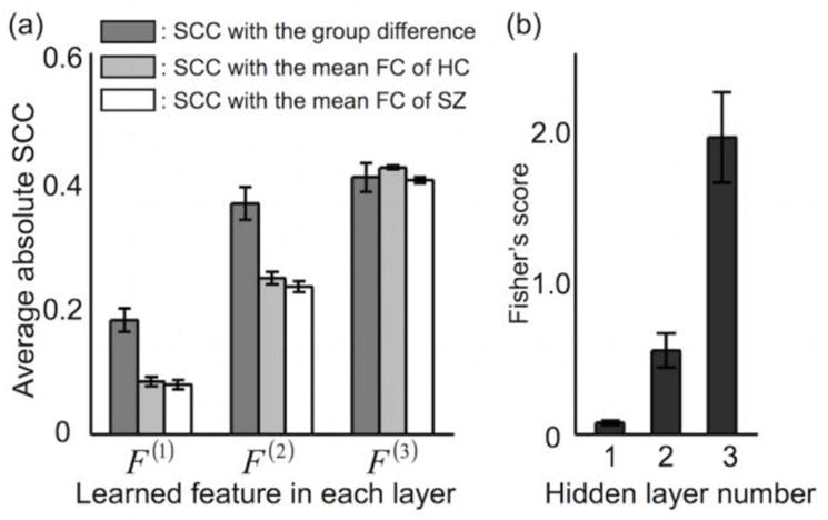
Quantitative evaluation of the learned hierarchical features across the hidden layers. (a) Absolute values of the spatial correlation coefficients (SCCs) using the learned features in each of the hidden layers and (b) Fisher’s scores across 50 hidden nodes in each of the hidden layers (both data sets, means ± the SD). F^(J) indicates the learned features in the J^th hidden layer. All measures were calculated from the trained deep neural network (DNN) with three hidden layers. FC, functional connectivity; SZ, schizophrenia; HC, healthy control.

Table S5 shows the kurtosis and modularity values of the DNN weights obtained for varying numbers of linearly combined weights. The estimated kurtosis values of the learned features for the first hidden layer (7.1 ± 0.9) were significantly greater than the kurtosis values of the second hidden layer (3.9 ± 0.4; Bonferroni-corrected p <10⁻⁴ from a two-sample t-test; d.f. = 98) and the third hidden layer (3.4 ± 0.2; Bonferroni-corrected p <10⁻⁴ from a two-sample t-test; d.f. = 98) when 15 DNN features in the lower layer were averaged to estimate the DNN feature in the higher layer. The average modularity values of the DNN features decreased from the lower to the higher layers. Across the hidden layers, the kurtosis values were more reproducible than the modularity values (ICC of 0.92 for kurtosis values vs. ICC of 0.44 for modularity values when the number of linearly combined weights/features was 15).

Classification performance for various parameter sets

Figure 12a illustrates the average learning curves, in which the proposed adaptive L₁-norm regularization β(t) along with pre-training initialization was superior in terms of final error rate and convergence speed compared with the fixed β. When β was fixed to 10⁻², the DNN weights during the DNN training diverged (i.e., the intensity of the DNN weights keeps increasing/decreasing). The adaptive β(t) method enabled a convergence (a) to a minimum error rate (compared with error rates from the fixed β of 10⁻³ and 10⁻⁴) and (b) to the target non-zero ratio (compared with the gradually decreasing non-zero ratio from the fixed β). A similar trend for the learning curves obtained from the adaptive β(t) and fixed β can be observed in the results using the random initialization of DNN weights, but with much higher error rates than the pre-training initialization of DNN weights (Fig. 12b). The average learning curves without pre-training (i.e., random initialization) suggested that the proposed adaptive β(t) was consistently better than the approach using a fixed β in terms of error rate (e.g., 20.2% with an adaptive β(t) vs. 24.3% with a fixed β of 10⁻³) and convergence speed (e.g., less than 500 epochs to converge with an adaptive β(t) vs. approximately 750 epochs to converge with a fixed β of 10⁻³) (Fig. 12b). Overall, the performance of the DNN without pre-training was inferior to that of the DNN with pre-training as evidenced by the greater error rate (20.2% vs. 14.2%) and slower convergence speed.

Figure 12.

Average learning curves (with SD) of error rates (first row) and the non-zero ratios (second row) from the first hidden layer (a) with pre-training and (b) without pre-training. The first column denotes the results from the proposed weight sparsity control via adaptation of the L₁-norm regularization parameter. The second, third, and fourth columns are the results from the fixed L₁-norm regularization parameter (10⁻², 10⁻³, and 10⁻⁴, respectively). SD, standard deviation.

Figure 13a shows that error rate obtained from an adaptive control of the L₁-norm regularization parameter (i.e., β(t)) to train the DNN with three hidden layers was 14.2 ± 0.4%, which is superior to the error rates (42.1 ± 1.7%, 18.2 ± 0.8%, and 20.1 ± 1.2% using 10⁻², 10⁻³, and 10⁻⁴, respectively) from the fixed L₁-norm regularization parameter (i.e., β). The L₂-norm regularization parameter γ had virtually no impact on classification performance as shown in Figure 13b. Figure 13c shows the classification performance depending on the numbers of hidden layers/nodes via a grid search, and the error rate was minimal (14.2%) when three hidden layers and 50 hidden nodes were used.

Figure 13.

Classification performance obtained from varying sets of parameters: (a) the proposed adaptive L₁-norm regularization parameter vs. several fixed L₁-norm regularization parameters, (b) the L₂-norm regularization parameters, and (c) a grid of the numbers of hidden layers and hidden nodes.

Classification performance bias due to framewise displacement

The average FD values from the HC (0.22 ± 0.09 mm) and SZ (0.28 ± 0.10 mm) groups were statistically different (Bonferroni-corrected p < 0.01 via a two-sample t-test; d.f. = 99). The higher-order momentum values (i.e., skewness and kurtosis) of the FC pattern before and after the FD removal are summarized in Table S6. Overall, the skewness and kurtosis values were significantly reduced after the FD removal, which indicated that the FC patterns were Gaussianized after the FD correction. There was no significant difference in these values between the two groups as measured using a two-sample t-test, and no significant interaction (group × FD) was detected using a two-way ANOVA (uncorrected p = 0.12). Figure 14 illustrates that the classification performance was slightly degraded by removing the FD component in the FC patterns, in which the error rates from the DNN classifier were 14.2 ± 0.4% and 16.6 ± 1.2% using the FC patterns with and without the FD removal, respectively. A similar trend was observed using SVM classifiers with the linear kernel (22.3 ± 0.8% and 26.6 ± 1.8%) and the RBF kernel (24.7 ± 1.3% and 24.9 ± 0.8%).

Figure 14.

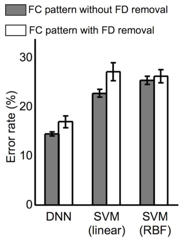
Classification performance obtained from the adopted classifiers (i.e., the DNN with three hidden layers and 50 nodes in each hidden layer; the SVM with linear or RBF kernels) using FC patterns with and without framewise displacement (FD) removal. DNN, deep neural network; SVM, support vector machine; RBF, radial basis function.

Classification performance using FC patterns of functionally parcellated brain regions from GICA

The 145 brain regions were functionally defined using the 145 ICs from the GICA (Fig. S4). The 126 ICs were predominantly located in the GM. Among these ICs, the TCs of the 116 ICs with greater proportions of voxels defined in the GM than those in the ten remaining ICs were further used to calculate the FC patterns. Figure 15a depicts the average error rates obtained from 50 randomly permuted training/validation/test data for each of the target non-zero ratios and for the DNNs with several numbers of hidden layers. The average error rate of the DNN with one hidden layer (24.1%) was lowest, and the optimal non-zero ratio was 0.4. For the DNN with three hidden layers, the average error rate was 13.5%, and the optimal non-zero ratios were 0.4, 0.6, and 0.7 from the first, second, and third hidden layers, respectively. Figure 15b shows the optimal (i.e., when the error rate was at its minimum) non-zero ratio for each of the hidden layers obtained via explicit control of the weight sparsity for each of the DNNs. Figure 15c shows that the error rates of 24.1 ± 0.7%, 16.4 ± 0.8%, 13.5 ± 1.2%, 15.1 ± 1.3%, and 17.6 ± 2.2% were achieved from the DNNs with one, two, three, four, and five hidden layers, respectively, whereas the error rates from the SVM with linear and RBF kernels were 23.1 ± 1.1% and 24.2 ± 1.2%, respectively.

Figure 15.

(a) Error rates for several target non-zero ratios using input FC patterns obtained from the GICA-based functional parcellation approach and using DNNs with several hidden layers. (b) The optimal (i.e., when average error rate evaluated across validation data was at the minimum) non-zero ratios for each of the DNNs (mean ± SD). (c) Minimum error rates from each of the DNNs with several numbers of hidden layers and from SVM classifiers with linear or RBF kernels. GICA, group independent component analysis; DNN, deep neural network; SD, standard deviation; RBF, radial basis function; ρ^(J+1,J), target non-zero ratio of W^(J+1,J); W^{(J+1, J)}, the DNN weights between the J^th and (J+1)^th layers.

Discussion

Study summary

In the present study, a DNN classifier trained with pre-training and explicit control of weight sparsity demonstrated significantly enhanced performance for the rsfMRI-facilitated automated diagnosis of SZ patients from HC subjects relative to the SVM classifier. The classification performance was systematically evaluated under various conditions, including (1) differing numbers of hidden layers and hidden nodes, (2) the presence or absence of adaptive L₁-norm regularization for weight sparsity control, (3) the presence or absence of SAE-based pre-training for weight initialization, (4) the presence or absence of FD regression to the FC patterns, and (5) anatomically or functionally defined ROIs to calculate the FC patterns.

The key findings of this investigation are summarized as follows: (1) the L₁-norm regularization of the DNN weights via explicit sparsity control improved the classification performance; (2) the SAE-based pre-training of DNN weights further enhanced classification performance; (3) the lower-to-higher level features of the whole-brain FC patterns were learned in the lower-to-higher layers of the DNN; and (4) lower-level/local features in the lower layer reflected aberrant FC pairs associated with SZ, whereas higher-level/global features in the higher layer represented FC alterations of SZ patients across the entire brain. The minimum error rate (14.2%) obtained from the DNN with three hidden layers employing both L₁-norm regularization and SAE-based pre-training was markedly decreased compared with the minimum error rate (28.1%) obtained from an earlier study using the same data set (albeit with slightly different included subjects) and the SVM-based classifier (Watanabe et al., 2014), as well as that obtained from the SVM classifier in the current study (22.3%).

Classification performance improvement from adaptive L₁-norm regularization and pre-training

Both L₁-norm regularization of the DNN weights via explicit sparsity control and SAE-based pre-training of the DNN weights contribute to the improved classification performance. Based on the results of a three-way ANOVA with three factors, including the use of sparsity control, use of pre-training, and the number of hidden layers of the DNN, the statistical significance of the interaction between the number of hidden layers and the use of pre-training (Bonferroni-corrected p < 10⁻⁷; d.f. = 499) was greater than that between the number of hidden layers and the use of sparsity control (Bonferroni-corrected p < 0.05; d.f. = 499). Pre-training benefitted DNNs with a greater number of hidden layers more than DNNs with a fewer number of hidden layers. L₁-norm regularization of the DNN weights can work as an efficient feature selection strategy that yields a sparse solution, particularly in the lower layer, to deal with high dimensionality of the input and intra-subject variability (Michel et al., 2012).

Efficacy of sparsity control of weights to DNN training

It is important to note that our proposed explicit control of the weight sparsity via application of the adaptive L₁-norm regularization parameter, β(t), improved the classification performance of the DNN by optimizing the sparsity level in each hidden layer through the use of non-zero ratios of the DNN weights during a training phase. On the other hand, the L₁-norm regularization parameter was fixed in previous studies (Kim et al., 2012; Watanabe et al., 2014). Thus, the scheme employed herein allowed a systematic evaluation of DNN classifier performance depending on the sparsity level of the weights for each hidden layer. Consequent results indicated that the error rate was more sensitive to the target non-zero ratios for the first hidden layer than to the ratios for the higher hidden layers, and that the error rate deviated less across the target non-zero ratios in the higher hidden layers (Figs. 6b–e).

The optimization criterion of the proposed DNN that incorporate both L₂-norm regularization and L₁-norm regularization were similar to those of the elastic net (Zou and Hastie, 2005) in the context of sparse feature extraction and dealing with highly correlated variables. However, there are distinctions between the elastic net and the proposed DNN, in which (1) our proposed regularization scheme is to adaptively update the L₁-norm regularization parameter explicitly to reach the target non-zero ratio, as opposed to the use of a constant regularization parameter in the elastic net, (2) optimization criteria with both L₁-norm and L₂-norm terms were extended to the multilayer networks of the DNN, and (3) the weight initialization was performed using an AE (stacked) in our DNN and using random initialization in an elastic net.

Importantly, an approach enforcing a sparsity level of the weights with L₁-norm regularization would not guarantee that the obtained weights (i.e., features) were correct and would, thus, potentially generate multiple false positives. Even for the simpler LASSO scheme, there is no statistical control over false positives since ground truth may not be available. In our study, the maximum validation accuracy in the CV phase was used as a ground truth to identify the optimal weight sparsity levels (i.e., assuming lower false positives at the optimal sparsity level) across the layers among several pre-defined candidates. The fine-tuning of the optimal sparsity level with increased number of candidate sparsity levels in each layer can be implemented at the expense of computational complexity. Future study is warranted to investigate the optimal sparsity level in each of the hidden layers in a more systematic manner than that presented, such as by controlling a smoothing parameter of the adaptive LASSO to reach a desired local false discovery rate (Sampson et al., 2013).

Spatial regularization, in addition to sparsity control, is necessary to include variable patterns across subjects. Thus, consideration of both sparsity control to deal with the intra-subject variability and spatial regularization to deal with the inter-subject variability may further improve the classification performance (Michel et al., 2012; Ng and Abugharbieh, 2011; Ng et al., 2012). As an example, Michel and colleagues (2012) reported that the sparsity in an individual subject enhances prediction accuracy because of the capability of finding sparse and fine-grained patterns.

Efficacy of SAE-based pre-training for DNNs

The adopted cost function of our DNN with multiple hidden layers may be highly non-convex in the parameter space, and multiple distinct local minima or plateaus would exist in the parameter space. The major challenge is that not all of these local minima provide equivalent classification errors, and a gradient descent learning method with random initialization may be trapped into severe local minima or plateaus (Bengio and LeCun, 2007). Initialization of the weights with SAE-based pre-training can be seen as a constraint, that. the weights represent the distribution of the input p(X_FC) modeled by an AE, where X_FC is an input FC pattern (Bengio et al., 2007). This initialization can work as a good starting point to maximize the conditional probability of the target vector of the class for a given input, p(t_class|X_FC) (Bengio et al., 2007). Since the supervised fine-tuning step of Eq. (2) was exactly the same for cases with and without pre-training, the performance degradation of random initialization compared with that of pre-training in our findings may provide empirical evidence in this context. The minimum error rates and lower variance in the error rates from the DNN with pre-training (14.2 ± 0.4%) compared with those using random initialization (20.2 ± 1.2%) in the adaptive L₁-norm regularization framework would support the assertion that the DNN with pre-training is more robust to the variability of samples than the DNN training with random initialization (Table 3). The results from the report showing that the unsupervised pre-training scheme is particularly well-suited when the supervised training data are limited (Deng and Yu, 2014) may well explain our findings. Accordingly, SAE-based pre-training can maximize classification performance using the whole-brain rsfMRI FC patterns, particularly for DNNs with multiple hidden layers.

Optimal parameters of adopted classifiers

The optimal non-zero ratio parameters for the DNNs with several numbers of hidden layers were reproducible across the permuted CV sets. The DNN with three hidden layers presented the maximum ICC value as well as the highest classification performance among the DNNs with several different numbers of hidden layers, indicating that this DNN is well-suited to our input data. Compared with the optimally selected parameter of the linear kernel SVM, the SVM with the RBF kernel represented a trade-off between the soft margin and RBF kernel size parameters.

Hierarchical feature representation of whole-brain FC patterns obtained from DNNs with sparsity control and pre-training

The linear combination of weights adopted in the present study is straightforward and efficient; however, this approach has potential limitations, including (1) an absence of an analytical guideline for the number of weights to be combined, and (2) a linear approximation of the nonlinear sigmoid function in each hidden node. This linear combination is proportional to the gradient update term of maximization of activation patterns of hidden nodes (Erhan et al., 2009). Using this feature representation, the lower-to-higher level features of the whole-brain rsfMRI data were extracted from the hidden layers of the DNN (Figs. 10, S1–S3). In DNNs presenting with the minimum error rates, the non-zero ratios were consistently smaller in the first hidden layer than in the higher hidden layers (Fig. 6f). This was also indicated by the sparsely formed FC features in the first hidden layer decomposed from the whole-brain FC patterns (Fig. 10, Table S5). The linear combination of these sparsely connected FC patterns can be interpreted as the integration of the aberrant FC levels that maximize the output of the hidden nodes at the higher layers (i.e., FC features that maximize the difference between the HC and SZ groups). According to the Fisher’s scores and the spatial CCs between the learned features and the t-scored group-level FC differences (Fig. 11), the trained weights of the higher hidden layers reflected inter-group differences and exhibited higher discriminative power than the lower hidden layers. Therefore, the learned features in the higher layers represent FC alterations in SZ patients distributed throughout the entire brain, which may implement the dysfunctional integration of aberrant “small-world” FC patterns (Liang et al., 2006; Liu et al., 2008).

Based on quantitative analysis of kurtosis, the learned features from the first hidden layer represent a super-Gaussian distribution (kurtosis value = 7.1 ± 0.9) when the number of the linearly combined weights is 15, while the learned features from the higher hidden layers approximate a Gaussian distribution (kurtosis values = 3.9 ± 0.4 and 3.4 ± 0.2 for the second and third hidden layers, respectively; Table S5). A graph theoretic modularity measure has been demonstrated the hierarchical characteristics of brain networks (Meunier et al., 2010). The greater degree of modularity from the first hidden layer than the higher hidden layers implies that whole-brain FC patterns are parcellated into several sub-modules at the first hidden layer and a nonlinear combination of these sub-modules at the higher hidden layer due to the sigmoid function of the hidden node, constituted a fully connected, large-scale FC network. Furthermore, the modularity of the learned DNN features was moderately consistent across several choices in number of the linearly combined weights, whereas the local to global layouts of the DNN features measured from the kurtosis values were highly reproducible across several choices in the number of linearly combined weights (Table S5).

Classification performance depending on various parameter sets

The classification performance from our proposed scheme to control the weight sparsity level via the adaptive L₁-norm regularization parameter β(t) using a target non-zero ratio of the DNN weights (i.e., minimum error rate of 14.2%) outperformed that of the fixed L₁-norm regularization parameter (i.e., 18.2% and 20.1% when β = 10⁻³ and 10⁻⁴, respectively). When β was fixed to 10⁻², the learning curves of the error rates kept increasing both with/without pre-training initialization, indicating that the DNN learning diverged. A stringent L₁-norm regularization of the DNN weights may prevent the minimization of the MSE cost function (Mohr et al., 2015). The classification performance was insensitive to the L₂-norm regularization parameter.

It appears that there is a trade-off in the DNN size, that is, the number of hidden layers vs. the number of nodes in each hidden layer. In our study, the optimal numbers of hidden layers and nodes in each hidden layer were investigated via a grid search using several candidate parameter values to prevent an exhaustive search of these parameters. Using our data, three hidden layers and 50 nodes in each hidden layer were chosen as an optimal size of the DNN (Fig. 13c). The classification performance kept increasing as the number of hidden layer was increased to three, whereas the classification performance was saturated/degraded for the DNNs with four/five hidden layers, respectively (Fig. 8) (Plis et al., 2014). The lower numbers of hidden layers/nodes may not be well suited to extract meaningful information hidden in the input sample dimension (i.e., 6670). Similarly, another empirical study on the number of hidden layers using an MNIST database with SAE-based pre-training demonstrated that the classification performance gradually increased when the number of hidden layers was increased to four and marginally deteriorated with five hidden layers (Erhan et al., 2010). The reason for this performance degradation would be due to the (1) increased number of parameters to train the DNN compared with the available number of input samples (Deng and Yu, 2014), (2) increased likelihood of finding poor local minima even after pre-training (Erhan et al., 2010), and (3) vanished or exploded gradient of a back-propagation algorithm as the number of hidden layers increased (Glorot and Bengio, 2010; Raiko et al., 2012). We believe that our proposed adaptive approach of weight sparsity control can alleviate the possibility of the solution getting stuck in poor local minima by reducing the number of non-zero parameters while maintaining the complexity of the network to extract meaningful information from lower-to-higher layers using complex whole-brain resting-state FC patterns. This may lead to the superior performance using our DNN compared with that using the SVM classifier.

Classification performance bias due to head motion

Based on recent reports, micromovements (e.g., a subtle head motion > 0.1 mm) have been significantly associated with regional BOLD signals identified using rsfMRI data (Van Dijk et al., 2012; Yan et al., 2013). Specifically, positive and negative motion-BOLD associations were found in the primary/supplementary motor and prefrontal areas, respectively (Yan et al., 2013), and a decreased coupling between head motion and FC levels was found in the DMN and fronto-parietal networks (Van Dijk et al., 2012). In our study, volume scrubbing and FD regression were used to minimize the effect of head motion on FC patterns in intra-subject and inter-subject/group levels and to reduce a potential bias on the classification performance which was degraded after the FD removal. Head motion at both the intra- and inter-subject levels must be carefully considered, particularly when groups composed of participants such as SZ patients tend to exhibit greater head movements in the raw fMRI data than the comparison group.

Brain volume registration/parcellation to define ROIs and functionally defined ROIs

The EPI volume registration and parcellation have long been a major issue (Ashburner, 2007; Klein et al., 2009). In our study, a normalization scheme using the subject’s EPI and an EPI template available in SPM8 was adopted to register the subject’s EPI volume into the MNI space and to assign each voxel to the ROIs in the AAL template. However, a normalization method using a high-resolution structural MRI with, in particular, the Diffeomorphic Anatomical Registration Through Exponentiated Lie Algebra (DARTEL), would further enhance the precision of the ROI definition. This may improve the specificity and sensitivity of the identified features associated with the SZ patients and, consequently, the classification performance. In addition to the structurally defined ROIs using brain volume registration, functionally defined ROIs has been proposed using various parcellation approaches such as hierarchical clustering and GICA approaches (Blumensath et al., 2013; Calhoun and Adali, 2012). For example, Blumensath and colleagues (2013) investigated an individual-level functional parcellation of the whole brain using a hierarchical clustering approach that enforces spatial contiguity of the parcels.

The FC patterns using the functionally defined ROIs from the GICA represented greater classification performance (i.e., error rates of 13.5 ± 1.2% using the DNN with three hidden layers) compared with that for the FC patterns using the anatomically defined ROIs from the AAL template (14.2 ± 0.4%; Bonferroni-corrected p < 10⁻³; d.f. = 99). In addition, the optimal non-zero ratios in the lower layer were slightly reduced (i.e., more sparse) using the FC patterns from the functionally defined brain regions (i.e., 0.41) compared with those obtained using the anatomically guided brain regions (i.e., 0.52). Thus, this may indicate that the GICA-based functional parcellation of brain regions provides more homogenous temporal patterns of neuronal activations via TCs of ICs than the average BOLD signal in each of the brain regions defined in the AAL template. Rigorous evaluations of our adopted GICA-based functional parcellation are warranted to address potential issues, such as an ambiguity in defining the total number of ICs to extract and the identification of non-neuronal components, including movements and brain edges (McKeown et al., 1998). Alternative options to functionally divide brain regions are available, such as using a variance-minimizing approach based on hierarchical agglomerative clustering or a spatially constrained spectral clustering approach (Craddock et al., 2012; Thirion et al., 2014).

Aberrant features of FC patterns in the first hidden layer

The learned features of the DNN weights between the input layer and the first hidden layer are in agreement with previous studies and include findings such as aberrant FC patterns between the thalamus and the cerebellum (Çetin et al., 2014; Collin et al., 2011; Magnotta et al., 2008) and between the frontal and the temporal areas, possibly due to auditory hallucinations (Martí-Bonmatí et al., 2007). The reduced FC level from SZ group between the precuneus/PCC and the striatum may indicate altered striatal dopaminergic functions (Dandash et al., 2013; Tu et al., 2012). The causal relationship of this connectivity requires further investigation.

DNN as a potential pattern classifier of neuroimaging data

How correlated features are handled is an important characteristic of a classifier. For example, a random forest deals with correlated features via subsampling for both the input sample and feature dimensions (Breiman, 2001). Empirical evidence suggests that the DNN can efficiently handle correlated features (Pan et al., 2012), although a rigorous theoretical derivation examining how it does so is warranted. For example, superior classification performance was found for input data of temporally concatenated and, thus, correlated speech frames using a DNN compared with that for input data of a single speech frame using the Gaussian mixture model, which cannot handle the correlated feature (Pan et al., 2012). Despite specific methodological differences, the DNN shares several important properties with the random forest. First, the semi-batch learning process with a randomized order of input samples for the DNN is similar to the subsampling of input samples for the random forest. Also, stochastic corruption of the input pattern via random zeroing of the DNN (Hinton et al., 2012; Vincent et al., 2010) is comparable to the subsampling of the feature dimension using the random forest. Finally, the weight sparsity control of our DNN may be analogous to the Gini index-based feature selection of the random forest, in which unimportant nodes have small values and vice versa (Qi, 2012).

In our study, the numbers of samples were balanced between the two groups (i.e., 50 subjects each in the HC and SZ groups), and the training/validation/test data were stratified in the nested CV framework to include balanced numbers of subjects from each of the two groups. With limited or imbalanced sample sizes, such as in neuroimaging or gene data, the classification performance can be severely biased. As a data-based method to deal with the class-imbalanced samples for classification, a bootstrap resampling approach can be successfully applied (He and Garcia, 2009; Leung et al., 2014; Lin and Chen, 2012). For example, Lin and Chen (2012) adopted bootstrap resampling with equal sample sizes for each class of gene data set, followed by a post-hoc modification of the SVM output values weighted by the number of samples in each class. This approach can also be used with the DNN classifier.

Considering the above practical guidelines and theoretical points of view, we suggest that the presented DNN classifier can also be applied to other neuropsychiatric disorders characterized by aberrant FC patterns (Anand et al., 2005; Barkhof et al., 2014; Li et al., 2002), such as attention deficit hyperactivity disorder (Castellanos et al., 2008; Tomasi and Volkow, 2012) and major depressive disorder (Berman et al., 2014; Kerestes et al., 2014). More importantly, the presented DNN classifier could be extended to separate patient groups that in some cases are difficult to diagnose correctly due to overlapping symptoms such as psychotic bipolar and SZ patients (Meda et al., 2012).

Classification performance in comparison with earlier reports using similar data sets

It would not be straightforward to directly compare our classification performance with that of several previous studies (Du et al., 2012; Shen et al., 2010; Silva et al., 2014). Despite similar data sets adopted in some studies (Du et al., 2012; Silva et al., 2014), discrepancies may exist, such as with the demographic information of participants and severity of disease in SZ patients, in addition to the input pattern of the classifier (i.e., whole-brain FC pattern in our study). For example, the SZ participants in our study and in the study by Shen et al. (2010) were described as having relatively mild (i.e., “mildly ill” with a PANSS score of 58.78 ± 14.35) and severe (i.e., “markedly ill” with a PANSS score of 80.06 ± 16.55) pathology (Leucht et al., 2005), respectively. Age differences between groups can influence the classification performance (Manza et al., 2015). In the study by Shen et al. (2010), the ages of the participants in the HC (39.4 ± 12.7) and SZ (31.5 ± 11.1) groups were significantly different (uncorrected p = 0.02, using a two-sample t-test), whereas the ages of the participants in the two groups in our study were not (HC, 35.9 ± 13.6 vs. SZ, 35.5 ± 11.9; uncorrected p > 0.05). Thus, this difference between the studies may affect classification performance. The dimensionality of the input sample used to build a classifier may also influence the classification performance. For example, the dimensionality of the input sample for the classifier was much smaller (i.e., 53 by applying a kernel PCA to spatial patterns of GICA) in the study by Du and colleagues (2012) than that in our study (i.e., 6,670 from a whole-brain FC). The classification performance may be limited when the number of input samples is more restricted than the number of adjustable free parameters as this was also evidenced from our classification performance depending on various numbers of hidden layers/nodes.

Classification using multimodal data can be gainfully adopted for classification of brain disorders such as SZ and Alzheimer’s disease (Kim and Lee, 2013; Sui et al., 2012). In a recent report, Silva and colleagues (2014) reviewed the tenth annual Machine Learning for Signal Processing competition on the schizophrenia classification challenge using multimodal neuroimaging data from fMRI (to estimate FNC patterns) and structural MRI (to extract GM density). Data was divided into a training set and a public and private test set (the private set was only evaluated after the competition was completed). The best performance on the public test data was 0.95, though the competition organizers summarized as an overall area under the receiver operating characteristic curve (AUC) measure including both public and private test data. The best classification performance for the overall AUC measure was 0.89 using a Gaussian process classifier with prior distribution scaled by a probit transformation (Silva et al., 2014; Solin and Sarkka, 2014).

Future work

In future explorations, a larger data set would undoubtedly augment the DNN classification accuracy, because the variety of characteristic features related to input FC patterns can be disentangled when an appropriate strategy for DNN training is employed (Bengio, 2013). Therefore, it will be important to explore whether the DNN classifier can benefit from a cohort of SZ patients and HC subjects acquired across multiple sites (Gollub et al., 2013). Such a multi-site investigation would enable greater optimization of the free parameters of the DNN classifier, including the number of hidden layers, the number of nodes in each hidden layer, L₁-/L₂-norm regularization parameters, and the number of epochs.

The SZ patients in the current data set were taking assorted antipsychotic drugs for at least six months at the time of fMRI scanning, with the exception of one subject. Given that FC patterns are apparently modulated by antipsychotic drug use (Alonso-Solís et al., 2012; Fornito et al., 2011), the use of the present DNN model for the automated classification/diagnosis of unmedicated patients (Schlagenhauf et al., 2014; Zarogianni et al., 2013) forms the subject of another prospective future study. Moreover, the computer-aided prediction of the prognosis of pharmaceutical SZ treatment as assessed by neurobehavioral scales (e.g., the PANSS) and consequent guidance of treatment selection in an individual basis (Guo et al., 2008) are crucial future applications of our DNN model.

Lastly, it will also be important to investigate whether a random sampling of hyper-parameters (Bergstra and Bengio, 2012) and iterative shrinkage-thresholding algorithms in the context of L₁- and L₂-norm regularization of DNN weights (Beck and Teboulle, 2009) would further enhance the classification performance.

Potential limitations of the current investigation

The DNN training described herein required an enormous amount of computational resources and time compared with the SVM training. For instance, a DNN classifier with three hidden layers necessitated a training time with the currently employed hardware system (comprising a Linux cluster system with 32 CPU cores with Intel Xeon processors of 2.9 GHz and 64 GB RAM for each core) of ~100-fold longer than that afforded by the SVM classifier (~3.3 days vs. 0.8 h). The extended training time would drastically be reduced by utilizing dedicated hardware systems such as using a graphic processing unit (GPU) with the cuda-convnet software package (code.google.com/p/cuda-convnet). Also, the Bayesian optimization to find hyper-parameters (e.g., L₁-norm regularization parameter in each layer) instead of a grid search can be adopted (Snoek et al., 2012). Specifically, Snoek and colleagues (2012) adopted the Bayesian framework to reduce the number of hyper-parameters to be estimated and presented an increased classification performance compared to that of the standard grid search approach.

Conclusions

The current study successfully demonstrated the feasibility of the DNN classifier toward the automated diagnosis of SZ patients by using resting-state whole-brain FC patterns as input patterns. The minimum error rate obtained from a DNN with three hidden layers was superior to that obtained from the SVM classifier. We believe that the presented DNN with the extensions of weight sparsity control and SAE-based pre-training will be useful for a better understanding of the neural basis of various neuropsychiatric disorders in addition to SZ that are associated with aberrant FC patterns, and, ultimately, for the development of improved computer-aided diagnosis tools in clinical and pre-clinical settings.

Highlights.

• Deep neural network (DNN) improves schizophrenia (SZ) classification performance.

• Sparsity control of weights via L₁-norm regularization increases performance.

• Stacked autoencoder pre-training of DNN weights further enhances performance.

• Lower/higher level features can be extracted from the DNN.

• Lower/higher level features show aberrant FC in the pairs-of-nodes/networks in SZ.

Abbreviations

AAL

automated anatomical labeling

AE

autoencoder

ANOVA

analysis of variance

AUC

area under the receiver operating characteristic curve

BOLD

blood-oxygenation-level-dependent

CC

correlation coefficient

CSF

cerebrospinal fluid

CV

cross validation

DARTEL

Diffeomorphic Anatomical Registration Through Exponentiated Lie Algebra

DMN

default-mode network

DNN

deep neural network

DSM

Diagnostic and Statistical Manual of Mental Disorders

EPI

echo-planar imaging

FC

functional connectivity

FNC

functional network connectivity

GICA

group independent component analysis

GM

gray matter

HC

healthy control

ICA

independent component analysis

IC

independent component

ICC

intra-class correlation coefficient

LASSO

least absolute shrinkage and selection operator

MNI

Montreal Neurological Institute

MNIST

Mixed National Institute of Standards and Technology

MSE

mean squared error

NITRC

Neuroimaging Informatics Tools and Resources Clearinghouse

PANSS

Positive and Negative Syndrome Scale

PCA

principal component analysis

PCC

posterior cingulate cortex

RBF

radial basis function

ROI

regions of interest

rsfMRI

resting-state functional magnetic resonance imaging

SAE

stacked autoencoder

SCID

Structured Clinical Interview for DSM Disorders

SD

standard deviation

SP

spatial pattern

SPM

Statistical Parametric Mapping

TC

time course

SVM

support vector machine

SZ

schizophrenia

TS

time series

WM

white matter

References

- Alonso-Solís A, Corripio I, de Castro-Manglano P, Duran-Sindreu S, Garcia-Garcia M, Proal E, Nuñez-Marín F, Soutullo C, Alvarez E, Gómez-Ansón B. Altered default network resting state functional connectivity in patients with a first episode of psychosis. Schizophrenia research. 2012;139:13–18. doi: 10.1016/j.schres.2012.05.005. [DOI] [PMC free article] [PubMed] [Google Scholar]
- Anand A, Li Y, Wang Y, Wu J, Gao S, Bukhari L, Mathews VP, Kalnin A, Lowe MJ. Activity and connectivity of brain mood regulating circuit in depression: a functional magnetic resonance study. Biological psychiatry. 2005;57:1079–1088. doi: 10.1016/j.biopsych.2005.02.021. [DOI] [PubMed] [Google Scholar]
- Arbabshirani MR, Kiehl KA, Pearlson GD, Calhoun VD. Classification of schizophrenia patients based on resting-state functional network connectivity. Frontiers in neuroscience. 2013;7 doi: 10.3389/fnins.2013.00133. [DOI] [PMC free article] [PubMed] [Google Scholar]
- Ashburner J. A fast diffeomorphic image registration algorithm. Neuroimage. 2007;38:95–113. doi: 10.1016/j.neuroimage.2007.07.007. [DOI] [PubMed] [Google Scholar]
- Barkhof F, Haller S, Rombouts SA. Resting-state functional MR imaging: a new window to the brain. Radiology. 2014;272:29–49. doi: 10.1148/radiol.14132388. [DOI] [PubMed] [Google Scholar]
- Beck A, Teboulle M. A fast iterative shrinkage-thresholding algorithm for linear inverse problems. SIAM Journal on Imaging Sciences. 2009;2:183–202. [Google Scholar]
- Beckmann CF, Smith SM. Tensorial extensions of independent component analysis for multisubject FMRI analysis. Neuroimage. 2005;25:294–311. doi: 10.1016/j.neuroimage.2004.10.043. [DOI] [PubMed] [Google Scholar]
- Bell AJ, Sejnowski TJ. An information-maximization approach to blind separation and blind deconvolution. Neural computation. 1995;7:1129–1159. doi: 10.1162/neco.1995.7.6.1129. [DOI] [PubMed] [Google Scholar]
- Bengio Y. Statistical Language and Speech Processing. Springer; 2013. Deep learning of representations: Looking forward; pp. 1–37. [Google Scholar]
- Bengio Y, Lamblin P, Popovici D, Larochelle H. Greedy layer-wise training of deep networks. Advances in neural information processing systems. 2007;19:153. [Google Scholar]
- Bengio Y, LeCun Y. Scaling learning algorithms towards AI. Large-scale kernel machines. 2007;34 [Google Scholar]
- Bergstra J, Bengio Y. Random search for hyper-parameter optimization. The Journal of Machine Learning Research. 2012;13:281–305. [Google Scholar]
- Berman MG, Misic B, Buschkuehl M, Kross E, Deldin PJ, Peltier S, Churchill NW, Jaeggi SM, Vakorin V, McIntosh AR, Jonides J. Does resting-state connectivity reflect depressive rumination? A tale of two analyses. Neuroimage. 2014;103C:267–279. doi: 10.1016/j.neuroimage.2014.09.027. [DOI] [PubMed] [Google Scholar]
- Bishop CM. Neural networks for pattern recognition. 1995. [Google Scholar]
- Blumensath T, Jbabdi S, Glasser MF, Van Essen DC, Ugurbil K, Behrens TE, Smith SM. Spatially constrained hierarchical parcellation of the brain with resting-state fMRI. Neuroimage. 2013;76:313–324. doi: 10.1016/j.neuroimage.2013.03.024. [DOI] [PMC free article] [PubMed] [Google Scholar]
- Breiman L. Random forests. Machine learning. 2001;45:5–32. [Google Scholar]
- Brosch T, Tam R. Medical Image Computing and Computer-Assisted Intervention–MICCAI. Vol. 2013. Springer; 2013. Manifold Learning of Brain MRIs by Deep Learning; pp. 633–640. [DOI] [PubMed] [Google Scholar]
- Bullmore E, Frangou S, Murray R. The dysplastic net hypothesis: an integration of developmental and dysconnectivity theories of schizophrenia. Schizophrenia research. 1997;28:143–156. doi: 10.1016/s0920-9964(97)00114-x. [DOI] [PubMed] [Google Scholar]
- Bullmore ET, Woodruff PW, Wright IC, Rabe-Hesketh S, Howard RJ, Shuriquie N, Murray RM. Does dysplasia cause anatomical dysconnectivity in schizophrenia? Schizophrenia research. 1998;30:127–135. doi: 10.1016/s0920-9964(97)00141-2. [DOI] [PubMed] [Google Scholar]
- Calhoun VD, Adali T. Multisubject independent component analysis of fMRI: a decade of intrinsic networks, default mode, and neurodiagnostic discovery. Biomedical Engineering, IEEE Reviews in. 2012;5:60–73. doi: 10.1109/RBME.2012.2211076. [DOI] [PMC free article] [PubMed] [Google Scholar]
- Calhoun VD, Adali T, Pearlson GD, Pekar JJ. A method for making group inferences from functional MRI data using independent component analysis. Hum Brain Mapp. 2001;14:140–151. doi: 10.1002/hbm.1048. [DOI] [PMC free article] [PubMed] [Google Scholar]
- Calhoun VD, Eichele T, Pearlson G. Functional brain networks in schizophrenia: a review. Frontiers in human neuroscience. 2009;3 doi: 10.3389/neuro.09.017.2009. [DOI] [PMC free article] [PubMed] [Google Scholar]
- Calhoun VD, Potluru VK, Phlypo R, Silva RF, Pearlmutter BA, Caprihan A, Plis SM, Adalı T. Independent component analysis for brain fMRI does indeed select for maximal independence. PloS one. 2013;8:e73309. doi: 10.1371/journal.pone.0073309. [DOI] [PMC free article] [PubMed] [Google Scholar]
- Calhoun VD, Sui J, Kiehl K, Turner J, Allen E, Pearlson G. Exploring the psychosis functional connectome: aberrant intrinsic networks in schizophrenia and bipolar disorder. Frontiers in psychiatry. 2011;2 doi: 10.3389/fpsyt.2011.00075. [DOI] [PMC free article] [PubMed] [Google Scholar]
- Cao H, Duan J, Lin D, Shugart YY, Calhoun V, Wang Y-P. Sparse representation-based biomarker selection for schizophrenia with integrated analysis of fMRI and SNPs. Neuroimage. 2014 doi: 10.1016/j.neuroimage.2014.01.021. [DOI] [PMC free article] [PubMed] [Google Scholar]
- Castellanos FX, Margulies DS, Kelly C, Uddin LQ, Ghaffari M, Kirsch A, Shaw D, Shehzad Z, Di Martino A, Biswal B. Cingulate-precuneus interactions: a new locus of dysfunction in adult attention-deficit/hyperactivity disorder. Biological psychiatry. 2008;63:332–337. doi: 10.1016/j.biopsych.2007.06.025. [DOI] [PMC free article] [PubMed] [Google Scholar]
- Çetin MS, Christensen F, Abbott CC, Stephen JM, Mayer AR, Cañive JM, Bustillo JR, Pearlson GD, Calhoun VD. Thalamus and posterior temporal lobe show greater internetwork connectivity at rest and across sensory paradigms in schizophrenia. Neuroimage. 2014;97:117–126. doi: 10.1016/j.neuroimage.2014.04.009. [DOI] [PMC free article] [PubMed] [Google Scholar]
- Chai XJ, Castanon AN, Ongur D, Whitfield-Gabrieli S. Anticorrelations in resting state networks without global signal regression. Neuroimage. 2012;59:1420–1428. doi: 10.1016/j.neuroimage.2011.08.048. [DOI] [PMC free article] [PubMed] [Google Scholar]
- Chang CC, Lin CJ. LIBSVM: a library for support vector machines. ACM Transactions on Intelligent Systems and Technology (TIST) 2011;2:27. [Google Scholar]
- Collin G, Pol HEH, Haijma SV, Cahn W, Kahn RS, van den Heuvel MP. Impaired cerebellar functional connectivity in schizophrenia patients and their healthy siblings. Frontiers in psychiatry. 2011;2 doi: 10.3389/fpsyt.2011.00073. [DOI] [PMC free article] [PubMed] [Google Scholar]
- Craddock RC, James GA, Holtzheimer PE, Hu XP, Mayberg HS. A whole brain fMRI atlas generated via spatially constrained spectral clustering. Hum Brain Mapp. 2012;33:1914–1928. doi: 10.1002/hbm.21333. [DOI] [PMC free article] [PubMed] [Google Scholar]
- Cristianini N, Shawe-Taylor J. An introduction to support vector machines and other kernel-based learning methods. Cambridge university press; 2000. [Google Scholar]
- Dandash O, Fornito A, Lee J, Keefe RS, Chee MW, Adcock RA, Pantelis C, Wood SJ, Harrison BJ. Altered striatal functional connectivity in subjects with an at-risk mental state for psychosis. Schizophrenia bulletin. 2013:sbt093. doi: 10.1093/schbul/sbt093. [DOI] [PMC free article] [PubMed] [Google Scholar]
- Darken C, Moody J. Note on learning rate schedules for stochastic optimization. DTIC Document 1992 [Google Scholar]
- Deng L, Yu D. Deep Learning: Methods and Applications. Now Publishers Incorporated; 2014. [Google Scholar]
- Denil M, Shakibi B, Dinh L, de Freitas N. Predicting parameters in deep learning. Advances in neural information processing systems. 2013:2148–2156. [Google Scholar]
- Du W, Calhoun VD, Li H, Ma S, Eichele T, Kiehl KA, Pearlson GD, Adali T. High classification accuracy for schizophrenia with rest and task fMRI data. Front Hum Neurosci. 2012;6 doi: 10.3389/fnhum.2012.00145. [DOI] [PMC free article] [PubMed] [Google Scholar]
- Erhan D, Bengio Y, Courville A, Manzagol PA, Vincent P, Bengio S. Why does unsupervised pre-training help deep learning? The Journal of Machine Learning Research. 2010;11:625–660. [Google Scholar]
- Erhan D, Bengio Y, Courville A, Vincent P. Dept IRO, Université de Montréal, Tech Rep. 2009. Visualizing higher-layer features of a deep network. [Google Scholar]
- First MB, Spitzer RL, Gibbon M, Williams JB. Structured Clinical Interview for DSM-IV® Axis I Disorders (SCID-I), Clinician Version, Administration Booklet. American Psychiatric Pub; 2012. [Google Scholar]
- Fornito A, Yoon J, Zalesky A, Bullmore ET, Carter CS. General and specific functional connectivity disturbances in first-episode schizophrenia during cognitive control performance. Biological psychiatry. 2011;70:64–72. doi: 10.1016/j.biopsych.2011.02.019. [DOI] [PMC free article] [PubMed] [Google Scholar]
- Friston KJ, Frith CD. Schizophrenia: a disconnection syndrome. Clin Neurosci. 1995;3:89–97. [PubMed] [Google Scholar]
- Girvan M, Newman ME. Community structure in social and biological networks. Proceedings of the National Academy of Sciences. 2002;99:7821–7826. doi: 10.1073/pnas.122653799. [DOI] [PMC free article] [PubMed] [Google Scholar]
- Glorot X, Bengio Y. Understanding the difficulty of training deep feedforward neural networks. International conference on artificial intelligence and statistics; 2010. pp. 249–256. [Google Scholar]
- Gollub RL, Shoemaker JM, King MD, White T, Ehrlich S, Sponheim SR, Clark VP, Turner JA, Mueller BA, Magnotta V. The MCIC collection: a shared repository of multimodal, multi-site brain image data from a clinical investigation of schizophrenia. Neuroinformatics. 2013;11:367–388. doi: 10.1007/s12021-013-9184-3. [DOI] [PMC free article] [PubMed] [Google Scholar]
- Graves A, Mohamed A-r, Hinton G. Speech recognition with deep recurrent neural networks. Acoustics, Speech and Signal Processing (ICASSP), 2013 IEEE International Conference on; IEEE; 2013. pp. 6645–6649. [Google Scholar]
- Greicius M. Resting-state functional connectivity in neuropsychiatric disorders. Current opinion in neurology. 2008;21:424–430. doi: 10.1097/WCO.0b013e328306f2c5. [DOI] [PubMed] [Google Scholar]
- Grosenick L, Klingenberg B, Katovich K, Knutson B, Taylor JE. Interpretable whole-brain prediction analysis with GraphNet. Neuroimage. 2013;72:304–321. doi: 10.1016/j.neuroimage.2012.12.062. [DOI] [PubMed] [Google Scholar]
- Guo Y, DuBois Bowman F, Kilts C. Predicting the brain response to treatment using a Bayesian hierarchical model with application to a study of schizophrenia. Hum Brain Mapp. 2008;29:1092–1109. doi: 10.1002/hbm.20450. [DOI] [PMC free article] [PubMed] [Google Scholar]
- He H, Garcia EA. Learning from imbalanced data. Knowledge and Data Engineering, IEEE Transactions on. 2009;21:1263–1284. [Google Scholar]
- Hinton G, Osindero S, Teh YW. A fast learning algorithm for deep belief nets. Neural computation. 2006;18:1527–1554. doi: 10.1162/neco.2006.18.7.1527. [DOI] [PubMed] [Google Scholar]
- Hinton GE, Srivastava N, Krizhevsky A, Sutskever I, Salakhutdinov RR. Improving neural networks by preventing co-adaptation of feature detectors. 2012 arXiv preprint arXiv:1207.0580. [Google Scholar]
- Hjelm RD, Calhoun VD, Salakhutdinov R, Allen EA, Adali T, Plis SM. Restricted Boltzmann machines for neuroimaging: An application in identifying intrinsic networks. Neuroimage. 2014;96:245–260. doi: 10.1016/j.neuroimage.2014.03.048. [DOI] [PMC free article] [PubMed] [Google Scholar]
- Hosseini SH, Hoeft F, Kesler SR. GAT: a graph-theoretical analysis toolbox for analyzing between-group differences in large-scale structural and functional brain networks. PloS one. 2012;7:e40709. doi: 10.1371/journal.pone.0040709. [DOI] [PMC free article] [PubMed] [Google Scholar]
- Jafri MJ, Pearlson GD, Stevens M, Calhoun VD. A method for functional network connectivity among spatially independent resting-state components in schizophrenia. Neuroimage. 2008;39:1666–1681. doi: 10.1016/j.neuroimage.2007.11.001. [DOI] [PMC free article] [PubMed] [Google Scholar]
- Kay S, Opler L, Fiszbein A. Positive and negative syndrome scale (PANSS) rating manual. San Rafael, Cal: Social and Behavioral Science Documents; 1987. [Google Scholar]
- Kerestes R, Davey CG, Stephanou K, Whittle S, Harrison BJ. Functional brain imaging studies of youth depression: A systematic review. Neuroimage Clin. 2014;4:209–231. doi: 10.1016/j.nicl.2013.11.009. [DOI] [PMC free article] [PubMed] [Google Scholar]
- Kim D-Y, Yoo S-S, Tegethoff M, Meinlschmidt G, Lee J-H. The inclusion of functional connectivity information into fMRI based neurofeedback improves its efficacy in the reduction of cigarette cravings. J Cogn Neurosci. 2015a doi: 10.1162/jocn_a_00802. In Press. [DOI] [PubMed] [Google Scholar]
- Kim HC, Yoo SS, Lee JH. Recursive approach of EEG-segment-based principal component analysis substantially reduces cryogenic pump artifacts in simultaneous EEG-fMRI data. Neuroimage. 2015b;104:437–451. doi: 10.1016/j.neuroimage.2014.09.049. [DOI] [PubMed] [Google Scholar]
- Kim J, Kim YH, Lee JH. Hippocampus-precuneus functional connectivity as an early sign of Alzheimer’s disease: a preliminary study using structural and functional magnetic resonance imaging data. Brain Res. 2013;1495:18–29. doi: 10.1016/j.brainres.2012.12.011. [DOI] [PubMed] [Google Scholar]
- Kim J, Lee JH. Integration of structural and functional magnetic resonance imaging improves mild cognitive impairment detection. Magn Reson Imaging. 2013;31:718–732. doi: 10.1016/j.mri.2012.11.009. [DOI] [PubMed] [Google Scholar]
- Kim YH, Kim J, Lee JH. Iterative approach of dual regression with a sparse prior enhances the performance of independent component analysis for group functional magnetic resonance imaging (fMRI) data. Neuroimage. 2012;63:1864–1889. doi: 10.1016/j.neuroimage.2012.08.055. [DOI] [PubMed] [Google Scholar]
- Klein A, Andersson J, Ardekani BA, Ashburner J, Avants B, Chiang MC, Christensen GE, Collins DL, Gee J, Hellier P, Song JH, Jenkinson M, Lepage C, Rueckert D, Thompson P, Vercauteren T, Woods RP, Mann JJ, Parsey RV. Evaluation of 14 nonlinear deformation algorithms applied to human brain MRI registration. Neuroimage. 2009;46:786–802. doi: 10.1016/j.neuroimage.2008.12.037. [DOI] [PMC free article] [PubMed] [Google Scholar]
- Koch GG. Intraclass correlation coefficient. Encyclopedia of statistical sciences 1982 [Google Scholar]
- Kong X-z, Zhen Z, Li X, Lu H-h, Wang R, Liu L, He Y, Zang Y, Liu J. Individual differences in impulsivity predict head motion during magnetic resonance imaging. PloS one. 2014;9:e104989. doi: 10.1371/journal.pone.0104989. [DOI] [PMC free article] [PubMed] [Google Scholar]
- Kriegeskorte N, Simmons WK, Bellgowan PS, Baker CI. Circular analysis in systems neuroscience: the dangers of double dipping. Nat Neurosci. 2009;12:535–540. doi: 10.1038/nn.2303. [DOI] [PMC free article] [PubMed] [Google Scholar]
- Krizhevsky A, Sutskever I, Hinton GE. Imagenet classification with deep convolutional neural networks. Advances in neural information processing systems. 2012:1097–1105. [Google Scholar]
- Larochelle H, Bengio Y, Louradour J, Lamblin P. Exploring strategies for training deep neural networks. The Journal of Machine Learning Research. 2009;10:1–40. [Google Scholar]
- Lee H, Ekanadham C, Ng AY. Sparse deep belief net model for visual area V2. Advances in neural information processing systems. 2008a:873–880. [Google Scholar]
- Lee JH, Lee TW, Jolesz FA, Yoo SS. Independent vector analysis (IVA): multivariate approach for fMRI group study. Neuroimage. 2008b;40:86–109. doi: 10.1016/j.neuroimage.2007.11.019. [DOI] [PubMed] [Google Scholar]
- Lee JH, Ryu J, Jolesz FA, Cho ZH, Yoo SS. Brain-machine interface via real-time fMRI: preliminary study on thought-controlled robotic arm. Neurosci Lett. 2009;450:1–6. doi: 10.1016/j.neulet.2008.11.024. [DOI] [PMC free article] [PubMed] [Google Scholar]
- Leucht S, Kane JM, Kissling W, Hamann J, Etschel E, Engel RR. What does the PANSS mean? Schizophrenia research. 2005;79:231–238. doi: 10.1016/j.schres.2005.04.008. [DOI] [PubMed] [Google Scholar]
- Leung MK, Xiong HY, Lee LJ, Frey BJ. Deep learning of the tissue-regulated splicing code. Bioinformatics. 2014;30:i121–i129. doi: 10.1093/bioinformatics/btu277. [DOI] [PMC free article] [PubMed] [Google Scholar]
- Li SJ, Li Z, Wu G, Zhang MJ, Franczak M, Antuono PG. Alzheimer Disease: Evaluation of a Functional MR Imaging Index as a Marker 1. Radiology. 2002;225:253–259. doi: 10.1148/radiol.2251011301. [DOI] [PubMed] [Google Scholar]
- Liang M, Zhou Y, Jiang T, Liu Z, Tian L, Liu H, Hao Y. Widespread functional disconnectivity in schizophrenia with resting-state functional magnetic resonance imaging. Neuroreport. 2006;17:209–213. doi: 10.1097/01.wnr.0000198434.06518.b8. [DOI] [PubMed] [Google Scholar]
- Lin W-J, Chen JJ. Class-imbalanced classifiers for high-dimensional data. Briefings in bioinformatics. 2012:bbs006. doi: 10.1093/bib/bbs006. [DOI] [PubMed] [Google Scholar]
- Liu Y, Liang M, Zhou Y, He Y, Hao Y, Song M, Yu C, Liu H, Liu Z, Jiang T. Disrupted small-world networks in schizophrenia. Brain. 2008;131:945–961. doi: 10.1093/brain/awn018. [DOI] [PubMed] [Google Scholar]
- Magnotta VA, Adix ML, Caprahan A, Lim K, Gollub R, Andreasen NC. Investigating connectivity between the cerebellum and thalamus in schizophrenia using diffusion tensor tractography: a pilot study. Psychiatry Research: Neuroimaging. 2008;163:193–200. doi: 10.1016/j.pscychresns.2007.10.005. [DOI] [PMC free article] [PubMed] [Google Scholar]
- Mann HB, Whitney DR. On a test of whether one of two random variables is stochastically larger than the other. The annals of mathematical statistics. 1947:50–60. [Google Scholar]
- Manza P, Zhang S, Hu S, Chao HH, Leung HC, Chiang-shan RL. The effects of age on resting state functional connectivity of the basal ganglia from young to middle adulthood. Neuroimage. 2015;107:311–322. doi: 10.1016/j.neuroimage.2014.12.016. [DOI] [PMC free article] [PubMed] [Google Scholar]
- Martí-Bonmatí L, Lull JJ, García-Martí G, Aguilar EJ, Moratal-Pérez D, Poyatos C, Robles M, Sanjuán J. Chronic Auditory Hallucinations in Schizophrenic Patients: MR Analysis of the Coincidence between Functional and Morphologic Abnormalities 1. Radiology. 2007;244:549–556. doi: 10.1148/radiol.2442060727. [DOI] [PubMed] [Google Scholar]
- McKeown MJ, Jung TP, Makeig S, Brown G, Kindermann SS, Lee TW, Sejnowski TJ. Spatially independent activity patterns in functional MRI data during the stroop color-naming task. Proc Natl Acad Sci U S A. 1998;95:803–810. doi: 10.1073/pnas.95.3.803. [DOI] [PMC free article] [PubMed] [Google Scholar]
- Meda SA, Gill A, Stevens MC, Lorenzoni RP, Glahn DC, Calhoun VD, Sweeney JA, Tamminga CA, Keshavan MS, Thaker G. Differences in resting-state fMRI functional network connectivity between schizophrenia and psychotic bipolar probands and their unaffected first-degree relatives. Biological psychiatry. 2012;71:881. doi: 10.1016/j.biopsych.2012.01.025. [DOI] [PMC free article] [PubMed] [Google Scholar]
- Meunier D, Lambiotte R, Bullmore ET. Modular and hierarchically modular organization of brain networks. Frontiers in neuroscience. 2010;4 doi: 10.3389/fnins.2010.00200. [DOI] [PMC free article] [PubMed] [Google Scholar]
- Michel V, Gramfort A, Eger E, Varoquaux G, Thirion B. Machine Learning and Interpretation in Neuroimaging. Springer; 2012. A comparative study of algorithms for intra-and inter-subjects fMRI decoding; pp. 1–8. [Google Scholar]
- Mingoia G, Wagner G, Langbein K, Maitra R, Smesny S, Dietzek M, Burmeister HP, Reichenbach JR, Schlösser RG, Gaser C. Default mode network activity in schizophrenia studied at resting state using probabilistic ICA. Schizophrenia research. 2012;138:143–149. doi: 10.1016/j.schres.2012.01.036. [DOI] [PubMed] [Google Scholar]
- Mohr H, Wolfensteller U, Frimmel S, Ruge H. Sparse regularization techniques provide novel insights into outcome integration processes. Neuroimage. 2015;104:163–176. doi: 10.1016/j.neuroimage.2014.10.025. [DOI] [PubMed] [Google Scholar]
- Moody J, Hanson S, Krogh A, Hertz JA. A simple weight decay can improve generalization. Advances in neural information processing systems. 1995;4:950–957. [Google Scholar]
- Newman ME, Girvan M. Finding and evaluating community structure in networks. Physical review E. 2004;69:026113. doi: 10.1103/PhysRevE.69.026113. [DOI] [PubMed] [Google Scholar]
- Ng B, Abugharbieh R. Information processing in medical imaging. Springer; 2011. Generalized sparse regularization with application to fMRI brain decoding; pp. 612–623. [DOI] [PubMed] [Google Scholar]
- Ng B, McKeown MJ, Abugharbieh R. Group replicator dynamics: A novel group-wise evolutionary approach for sparse brain network detection. Medical Imaging, IEEE Transactions on. 2012;31:576–585. doi: 10.1109/TMI.2011.2173699. [DOI] [PubMed] [Google Scholar]
- Pan J, Liu C, Wang Z, Hu Y, Jiang H. Investigation of deep neural networks (DNN) for large vocabulary continuous speech recognition: Why DNN surpasses GMMS in acoustic modeling. ISCSLP. 2012:301–305. [Google Scholar]
- Plis SM, Hjelm D, Salakhutdinov R, Allen EA, Bockholt HJ, Long JD, Johnson HJ, Paulsen J, Turner JA, Calhoun VD. Deep learning for neuroimaging: a validation study. Frontiers in neuroscience. 2014;8 doi: 10.3389/fnins.2014.00229. [DOI] [PMC free article] [PubMed] [Google Scholar]
- Power JD, Barnes KA, Snyder AZ, Schlaggar BL, Petersen SE. Spurious but systematic correlations in functional connectivity MRI networks arise from subject motion. Neuroimage. 2012;59:2142–2154. doi: 10.1016/j.neuroimage.2011.10.018. [DOI] [PMC free article] [PubMed] [Google Scholar]
- Qi Y. Ensemble machine learning. Springer; 2012. Random forest for bioinformatics; pp. 307–323. [Google Scholar]
- Raiko T, Valpola H, LeCun Y. Deep learning made easier by linear transformations in perceptrons. International Conference on Artificial Intelligence and Statistics; 2012. pp. 924–932. [Google Scholar]
- Rosner B. Cengage Learning. 2010. Fundamentals of biostatistics. [Google Scholar]
- Salvador R, Suckling J, Coleman MR, Pickard JD, Menon D, Bullmore E. Neurophysiological architecture of functional magnetic resonance images of human brain. Cerebral cortex. 2005;15:1332–1342. doi: 10.1093/cercor/bhi016. [DOI] [PubMed] [Google Scholar]
- Sampson JN, Chatterjee N, Carroll RJ, Müller S. Controlling the local false discovery rate in the adaptive Lasso. Biostatistics. 2013;14:653–666. doi: 10.1093/biostatistics/kxt008. [DOI] [PMC free article] [PubMed] [Google Scholar]
- Schlagenhauf F, Huys QJ, Deserno L, Rapp MA, Beck A, Heinze HJ, Dolan R, Heinz A. Striatal dysfunction during reversal learning in unmedicated schizophrenia patients. Neuroimage. 2014;89:171–180. doi: 10.1016/j.neuroimage.2013.11.034. [DOI] [PMC free article] [PubMed] [Google Scholar]
- Schmidhuber J. Deep Learning in Neural Networks: An Overview. 2014 doi: 10.1016/j.neunet.2014.09.003. arXiv preprint arXiv:1404.7828. [DOI] [PubMed] [Google Scholar]
- Scott A, Courtney W, Wood D, De la Garza R, Lane S, King M, Wang R, Roberts J, Turner JA, Calhoun VD. COINS: an innovative informatics and neuroimaging tool suite built for large heterogeneous datasets. Frontiers in neuroinformatics. 2011;5 doi: 10.3389/fninf.2011.00033. [DOI] [PMC free article] [PubMed] [Google Scholar]
- Shen H, Wang L, Liu Y, Hu D. Discriminative analysis of resting-state functional connectivity patterns of schizophrenia using low dimensional embedding of fMRI. Neuroimage. 2010;49:3110–3121. doi: 10.1016/j.neuroimage.2009.11.011. [DOI] [PubMed] [Google Scholar]
- Silva RF, Castro E, Gupta CN, Cetin M, Arbabshirani M, Potluru VK, Plis SM, Calhoun VD. The tenth annual MLSP competition: Schizophrenia classification challenge. Machine Learning for Signal Processing (MLSP), 2014 IEEE International Workshop on; IEEE; 2014. pp. 1–6. [Google Scholar]
- Snoek J, Larochelle H, Adams RP. Practical Bayesian optimization of machine learning algorithms. Advances in neural information processing systems. 2012:2951–2959. [Google Scholar]
- Solin A, Sarkka S. The 10th annual MLSP competition: First place. Machine Learning for Signal Processing (MLSP), 2014 IEEE International Workshop on; IEEE; 2014. pp. 1–3. [Google Scholar]
- Song XW, Dong ZY, Long XY, Li SF, Zuo XN, Zhu CZ, He Y, Yan CG, Zang YF. REST: a toolkit for resting-state functional magnetic resonance imaging data processing. PLoS One. 2011;6:e25031. doi: 10.1371/journal.pone.0025031. [DOI] [PMC free article] [PubMed] [Google Scholar]
- Sui J, Yu Q, He H, Pearlson GD, Calhoun VD. A selective review of multimodal fusion methods in schizophrenia. Frontiers in human neuroscience. 2012;6 doi: 10.3389/fnhum.2012.00027. [DOI] [PMC free article] [PubMed] [Google Scholar]
- Suk H-I, Lee S-W, Shen D. Latent feature representation with stacked auto-encoder for AD/MCI diagnosis. Brain Structure and Function. 2013:1–19. doi: 10.1007/s00429-013-0687-3. [DOI] [PMC free article] [PubMed] [Google Scholar]
- Suk H-I, Lee S-W, Shen D. Hierarchical Feature Representation and Multimodal Fusion with Deep Learning for AD/MCI Diagnosis. Neuroimage. 2014 doi: 10.1016/j.neuroimage.2014.06.077. [DOI] [PMC free article] [PubMed] [Google Scholar]
- Tang Y, Wang L, Cao F, Tan L. Identify schizophrenia using resting-state functional connectivity: an exploratory research and analysis. Biomed Eng Online. 2012;11:50. doi: 10.1186/1475-925X-11-50. [DOI] [PMC free article] [PubMed] [Google Scholar]
- Thirion B, Varoquaux G, Dohmatob E, Poline J-B. Which fMRI clustering gives good brain parcellations? Frontiers in neuroscience. 2014;8 doi: 10.3389/fnins.2014.00167. [DOI] [PMC free article] [PubMed] [Google Scholar]
- Tomasi D, Volkow ND. Abnormal functional connectivity in children with attention-deficit/hyperactivity disorder. Biological psychiatry. 2012;71:443–450. doi: 10.1016/j.biopsych.2011.11.003. [DOI] [PMC free article] [PubMed] [Google Scholar]
- Tu PC, Hsieh JC, Li CT, Bai YM, Su TP. Cortico-striatal disconnection within the cingulo-opercular network in schizophrenia revealed by intrinsic functional connectivity analysis: a resting fMRI study. Neuroimage. 2012;59:238–247. doi: 10.1016/j.neuroimage.2011.07.086. [DOI] [PubMed] [Google Scholar]
- Tzourio-Mazoyer N, Landeau B, Papathanassiou D, Crivello F, Etard O, Delcroix N, Mazoyer B, Joliot M. Automated anatomical labeling of activations in SPM using a macroscopic anatomical parcellation of the MNI MRI single-subject brain. Neuroimage. 2002;15:273–289. doi: 10.1006/nimg.2001.0978. [DOI] [PubMed] [Google Scholar]
- Van Dijk KR, Sabuncu MR, Buckner RL. The influence of head motion on intrinsic functional connectivity MRI. Neuroimage. 2012;59:431–438. doi: 10.1016/j.neuroimage.2011.07.044. [DOI] [PMC free article] [PubMed] [Google Scholar]
- Venegas J, Clark E. Encyclopedia of Clinical Neuropsychology. Springer; 2011. Wechsler Test of Adult Reading; pp. 2693–2694. [Google Scholar]
- Vincent P, Larochelle H, Lajoie I, Bengio Y, Manzagol PA. Stacked denoising autoencoders: Learning useful representations in a deep network with a local denoising criterion. The Journal of Machine Learning Research. 2010;11:3371–3408. [Google Scholar]
- Watanabe T, Kessler D, Scott C, Angstadt M, Sripada C. Disease prediction based on functional connectomes using a scalable and spatially-informed support vector machine. Neuroimage. 2014;96:183–202. doi: 10.1016/j.neuroimage.2014.03.067. [DOI] [PMC free article] [PubMed] [Google Scholar]
- Wechsler D. Wechsler abbreviated scale of intelligence. Psychological Corporation; 1999. [Google Scholar]
- Xia M, Wang J, He Y. BrainNet Viewer: a network visualization tool for human brain connectomics. PloS one. 2013;8:e68910. doi: 10.1371/journal.pone.0068910. [DOI] [PMC free article] [PubMed] [Google Scholar]
- Yan CG, Cheung B, Kelly C, Colcombe S, Craddock RC, Di Martino A, Li Q, Zuo XN, Castellanos FX, Milham MP. A comprehensive assessment of regional variation in the impact of head micromovements on functional connectomics. Neuroimage. 2013;76:183–201. doi: 10.1016/j.neuroimage.2013.03.004. [DOI] [PMC free article] [PubMed] [Google Scholar]
- Yu Q, Allen AE, Sui J, Arbabshirani RM, Pearlson G, Calhoun DV. Brain connectivity networks in schizophrenia underlying resting state functional magnetic resonance imaging. Current topics in medicinal chemistry. 2012;12:2415–2425. doi: 10.2174/156802612805289890. [DOI] [PMC free article] [PubMed] [Google Scholar]
- Zarogianni E, Moorhead TW, Lawrie SM. Towards the identification of imaging biomarkers in schizophrenia, using multivariate pattern classification at a single-subject level. NeuroImage: Clinical. 2013;3:279–289. doi: 10.1016/j.nicl.2013.09.003. [DOI] [PMC free article] [PubMed] [Google Scholar]
- Zhou Y, Liang M, Tian L, Wang K, Hao Y, Liu H, Liu Z, Jiang T. Functional disintegration in paranoid schizophrenia using resting-state fMRI. Schizophrenia research. 2007;97:194–205. doi: 10.1016/j.schres.2007.05.029. [DOI] [PubMed] [Google Scholar]
- Zou H, Hastie T. Regularization and variable selection via the elastic net. Journal of the Royal Statistical Society: Series B (Statistical Methodology) 2005;67:301–320. [Google Scholar]
Associated Data
This section collects any data citations, data availability statements, or supplementary materials included in this article.