Bayesian network approach for modeling local failure in lung cancer

Abstract

Locally advanced non-small cell lung cancer (NSCLC) patients suffer from a high local failure rate following radiotherapy. Despite many efforts to develop new dose-volume models for early detection of tumor local failure, there was no reported significant improvement in their application prospectively. Based on recent studies of biomarker proteins’ role in hypoxia and inflammation in predicting tumor response to radiotherapy, we hypothesize that combining physical and biological factors with a suitable framework could improve the overall prediction. To test this hypothesis, we propose a graphical Bayesian network framework for predicting local failure in lung cancer. The proposed approach was tested using two different datasets of locally advanced NSCLC patients treated with radiotherapy. The first dataset was collected retrospectively, which is comprised of clinical and dosimetric variables only. The second dataset was collected prospectively in which in addition to clinical and dosimetric information, blood was drawn from the patients at various time points to extract candidate biomarkers as well. Our preliminary results show that the proposed method can be used as an efficient method to develop predictive models of local failure in these patients and to interpret relationships among the different variables in the models. We also demonstrate the potential use of heterogenous physical and biological variables to improve the model prediction. With the first dataset, we achieved better performance compared with competing Bayesian-based classifiers. With the second dataset, the combined model had a slightly higher performance compared to individual physical and biological models, with the biological variables making the largest contribution. Our preliminary results highlight the potential of the proposed integrated approach for predicting post-radiotherapy local failure in NSCLC patients.

1. Introduction

Lung cancer is a leading cause of cancer death in both men and women worldwide (American Cancer Society 2008). Of all lung cancer cases, approximately 80% are classified as non-small cell lung cancer (NSCLC). About 25% to 40% of NSCLC patients are in locally advanced stage III upon diagnosis (Choy et al 2005). For these patients with advanced and inoperable stage, a combination of chemotherapy and radiotherapy is used as the main treatment instead of surgical resection (American Cancer Society 2008). Local failure is a major issue in the treatment of patients with locally advanced NSCLC following radiotherapy (Armstrong et al 1995). Despite many efforts to improve treatment outcomes, however, a low two-year local control rate as low as 27% in these patients urgently requires innovative diagnostic and prognostic models to improve stratification of patients into different risk groups of patients who may need less than the standard dose, thus less toxicity, or of patients who may need a more intensive therapy, yet possibly more toxicity, to achieve local control (Abramyuk et al 2009).

In our previous works (Mu et al 2008, El Naqa et al 2010), we have used various approaches to extract relevant dose-volume metrics and evaluated linear and nonlinear models to predict tumor local control. In this work, we propose a novel Bayesian network framework for modeling local failure for patients with locally advanced NSCLC. A Bayesian network can be a useful tool to create individualized predictive models due to several attractive characteristics: (1) it provides ability to approximate complex multivariable probability distributions of heterogeneous variables as interpretable local probability distributions; (2) it can incorporate prior clinical and biological knowledge; (3) it enables easy visualization and interpretation of interactions among variables of interest for clinical use; and (4) it can be also used as a classifier based on a learned network structure. These characteristics have led to various studies increasingly using this technology in the oncology field. Recently, Jayasurya et al (2010) proposed a Bayesian network model for survival prediction in lung cancer patients. They also showed that the Bayesian network can be efficiently used when handling missing data compared with other learning techniques. Velikova et al (2009) designed a multi-view mammographic analysis system using a Bayesian network framework to detect breast cancer at patient level and demonstrated the potential of the system for selecting the most suspicious cases. Chen et al (2006) proposed an effective Bayesian structure learning method based on the mutual information and K2 algorithm to reconstruct reliable gene networks. van Gerven et al (2008) demonstrated the development of a prognostic model for carcinoid patients using dynamic Bayesian networks. Armañanzas et al (2008) used a hierarchical Bayesian structure learning method to detect gene interactions. Smith et al (2009) developed a prognostic model for prostate cancer with intensity modulated radiation therapy (IMRT) plans and calculated a quality-adjusted life expectancy for each plan using Bayesian networks.

The aim of this study is to develop an efficient method for Bayesian structure learning that can be used to predict local failure in lung cancer post-radiotherapy treatment. Our proposed method was tested with two different datasets. We show that the proposed method outperforms classical Bayesian-based classifiers and that incorporating physical and biological factors into the Bayesian network can further improve the predictive power. It is our expectation that the proposed model will provide physicians with an interpretable tool for better prediction of early recurrence in lung cancer and lead to more individualized radiotherapy prescriptions.

The remainder of this paper is organized as follows. In the following section, we briefly review the concept of Bayesian network analysis. In section 3, we describe the datasets used in this study and our proposed method for Bayesian network structure learning. The experimental results including comparisons with other Bayesian-based algorithms are presented in section 4. We finalize our work with discussion and conclusions in sections 5 and 6.

2. Bayesian network

A Bayesian network is a probabilistic graphical model that encodes a joint probability distribution among variables of interest (Sarkar and Boyer 1993, Heckerman and Breese 1996, Friedman et al 1997, Lucas 2005). A Bayesian network forms a directed-acyclic graph (DAG) by a set of nodes (representing the variables) and a set of directed edges (representing relationships among the variables). Given n variables, X = {X₁, X₂, ···, X_n}, the joint probability distribution can be decomposed into a product form of conditional probability distributions:

$$P(X)=\prod _{i=1}^{n}P(X_i\mid Pa(X_i))$$ (1)

where P a(X_i) indicates the set of parents of X_i in the Bayesian network.

Learning a Bayesian network structure is a task to find a DAG that best represents the dataset. This process consists of two main components: a scoring function and a search strategy (Chen et al 2006). The scoring function is used to evaluate how well the Bayesian structure represents the dataset. Given a scoring function, the goal is to identify the highest-scoring Bayesian network structure among all possible network structures, which amounts to a search problem. In Bayesian structure learning, however, a challenging problem is that the search space increases super-exponentially as the number of nodes increases, usually resulting in an NP-hard problem. Therefore, since an exhaustive search is not practicable, heuristic search strategies, including hill climbing and K2 are alternatively utilized. The K2 algorithm employs a greedy search strategy, which dramatically reduces the computational complexity in learning the Bayesian network structure by using a prior ordering of all the nodes (Cooper and Herskovits 1992). Therefore, following a K2 strategy, the key to successful Bayesian structure learning lies in choosing a correct node ordering.

3. Materials and methods

In this study, we tested the proposed Bayesian structure learning method with two different datasets collected at Mallinckrodt Institute of Radiology. The description of the datasets is followed by our proposed approach.

3.1. Local control

The clinical endpoint chosen for the study was local control. Following our institutional guidelines, patients were considered to have local control of disease if they had an initial radiographic response on CT images to treatment and a stable mass at each follow-up visit. Otherwise, patients were considered to have local failure if clinical, radiographic, or biopsy evidence of progression was observed. A minimum follow-up of six months was used.

3.2. Dataset A

This dataset consists of 56 NSCLC patients who received 3D conformal radiation therapy with a median prescription dose of 70 Gy (60–84 Gy) as part of their treatment and had a median follow-up of 32 months. Nine patients received sequential chemotherapy and 14 received concurrent chemotherapy. The patients were treated between March 1991 and December 2001 and were included in the study if they had complete treatment planning and follow-up records, at least six months of follow-up, and a discrete primary tumor exclusive of nodal regions. The original treatment plans were homogeneous with dose calculated to water, therefore, Monte Carlo simulations were used to correct the dose distributions for tissue heterogeneity (Lindsay et al 2007). With observations throughout a median follow-up period of 16 months for the endpoint of local control, the patients were divided into a local failure group (n = 22) and a control group (n = 34). In our previous work (El Naqa et al 2010), we used logistic regression with resampling methods to extract top five predictive models of tumor local control, each of which consisted of two variables, with the highest frequency on bootstrap analysis.

Coalescing these models resulted in the following five variables: the volume receiving at least 60 Gy (V60), the volume receiving at least 75 Gy (V75), PreTxChemo (indicating whether or not a patient received a chemotherapy before radiotherapy), gross tumor volume (GTV), and age. We used these five variables to test the proposed Bayesian structure learning method, whose values were extracted using our in-house software (DREES: dose-response explorer system) (El Naqa et al 2006b).

3.3. Dataset B

This dataset was collected prospectively and was approved by the Human Research Protection Office at our institute. The patients were not surgical candidates and had a discrete primary tumor (stage IIIb). In the study protocol, blood sera were drawn at pre-treatment and mid-treatment of radiotherapy NSCLC patients in addition to collecting clinical and dosimetric variables as in Dataset A. A total of 18 patients were evaluable for the current study. Three patients received sequential chemotherapy and 15 received concurrent chemotherapy. This dataset allows for unique integration of physical and biological variables. After post-evaluation throughout a median follow-up period of 16 months, the patients were divided into a local failure group (n = 8) and a control group (n = 10). With this dataset, the goal is to investigate and analyze interactions among heterogeneous physical and biological variables and to evaluate the complementary role of these variables in improving the prediction of tumor local control in NSCLC patients post-radiotherapy treatment.

This dataset included four selected biomarker proteins besides the physical variables described above. The biomarkers were selected because of their potential role in tumor response in lung cancer as described in literatures below. The four chosen biomarker proteins are as follows: transforming growth factor β (TGF-β), interleukin-6 (IL-6), angiotensin converting enzyme (ACE), and osteopontin (OPN). As mentioned earlier, these blood-based candidate proteins were selected based on previous reports linking their serum expression to tumor response post-radiotherapy treatment. Serum levels of ACE have been associated with poor prognosis in NSCLC, which is believed to be involved in the induction of apoptosis by TNF-α pathway (Varela and Saez 1993). In a recent study, OPN in serum has been shown to be a good correlate of tumor hypoxia and a significant prognostic factor of relapse risk (Le et al 2006). In addition, Rübe et al (2008) have reported that circulating cytokines (IL-6 and TGF-β1) in patients receiving radiotherapy for advanced NSCLC showed higher correlation with tumor response rather than lung inflammation contrary to what was previously reported. We measured expressions of these proteins using enzyme-linked immunosorbent assay (ELISA). As physical variables, two variables (V75 and GTV) were chosen from the top model in our previous study (refer to Section 3.2). In addition, tumor regression volume on 4D-CT images between pre-treatment and mid-treatment was measured using an active contour tracking algorithm (El Naqa et al 2008). Figure 1 shows two snapshots of pre-treatment tumor contour and mid-treatment contour estimated by the tracking algorithm using end-of-exhalation 4D-CT data.

Figure 1.

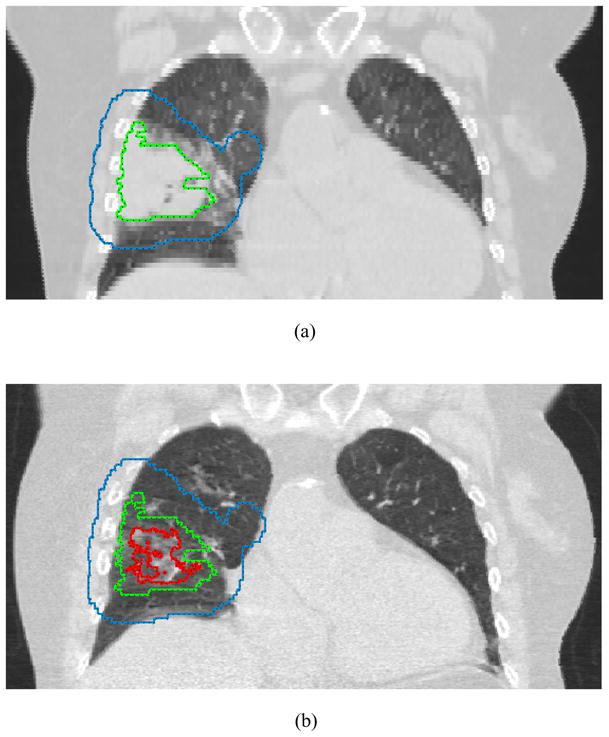
Snapshots taken from our in-house software (CERR). Contours represent planning target volume (blue), initial gross tumor volume (green), and shrinkage of gross tumor volume (red).

3.4. Preprocessing

In general, for Bayesian structure learning and evaluation of Bayesian classifiers, variables are discretized into two or three bins. For the determination of discretization boundaries, researchers have used the mean and standard deviation or the equal width. In both cases, however, it is difficult to find the optimal boundaries. Recently, Kuschner et al (2010) proposed an efficient binning method based on mutual information using a three-bin strategy, where bin boundaries are determined such that the mutual information of each variable given the treatment response class is maximized. As a result, each variable is discretized into three bins: high, medium, and low. For example, in discretizing the expression of a protein, the medium bin provides little or no discrimination between tumor recurrence and tumor control while the high and low bins show a large difference between the two groups. We applied the same approach for discretization to our datasets except for the class variable that is binary.

Mutual information is a measure of the mutual dependence of two random variables (for example, a class label (tumor recurrence or control) and a protein’s abundance). For two discrete random variables X and Y, the mutual information between them is defined mathematically as

$$I(X;Y)=\sum _{x\in X}\sum _{y\in Y}P(x,y)log\frac{P(x,y)}{P(x)P(y)}$$ (2)

where x and y represent all the possible values in X and Y, respectively, and P (x, y) represents the joint probability on the values x and y (Kuschner et al 2010).

3.5. Markov Chain Monte Carlo (MCMC) algorithm

To efficiently search the space of Bayesian network structures, a Markov Chain Monte Carlo (MCMC) method based on the Metropolis-Hastings algorithm was applied using the Bayes Net Toolbox (BNT) for Matlab, which rapidly converges to a locally optimal structure (Murphy 2007). We accumulated the Bayesian structure information of each MCMC run as follows. Let e_ij be the arc from variable X_i to variable X_j. Then, we define a_ijk as

$$a_{\mathit{ijk}}=\{\begin{array}{ll}1\hfill & \text{if}{e}_{ij}\text{is}\text{present}\text{in}\text{the}k\text{th}\text{MCMC}\text{run},\hfill \\ 0\hfill & \text{otherwise}.\hfill \end{array}$$ (3)

The number of occurrences of an arc e_ij over m runs of MCMC is

$$f_{ij}=\sum _{k=1}^m{a}_{\mathit{ijk}}.$$ (4)

Therefore, a matrix M that contains the number of occurrences for all edges can be expressed as

$$M=\left[\begin{array}{cccc}0& f_{12}& \dots & f_{1n}\\ f_{21}& 0& \dots & f_{2n}\\ & & ⋮& \\ f_{n1}& f_{n2}& \dots & 0\end{array}\right].$$ (5)

3.6. Maximum spanning tree

After several runs of MCMC algorithm, a weighted directed graph represented by the matrix M was populated. We applied a directed maximum spanning tree algorithm based on Chu-Liu/Edmonds’s algorithm to the weighted directed graph (Chu and Liu 1965, Edmonds 1967). As a result, a directed graph was obtained, from which we gained a node ordering that can be used as an input to the K2 algorithm. Specifically, from a weighted directed graph G = (V, E) where V is the set of nodes and E is the set of possible edges between pairs of nodes, and there is a weight w(u, v) for each edge (u, v) ∈ E, a directed maximum spanning tree is found such that the total weight of an acyclic subset T ⊆ E that connects all the nodes

$$w(T)=\sum _{(u,v)\in T}w(u,v)$$ (6)

is maximized. Figure 2 illustrates an example of the use of a directed maximum spanning tree algorithm.

Figure 2.

A directed maximum spanning tree that starts from a node s. The bold lines indicate the edges in a directed maximum spanning tree. The total weight of the tree shown is 96: w = w_s1 + w_s2 + w₂₅ + w₅₃ + w₅₄=30+5+4+27+30=96. The node order is [s,1,2,5,3,4].

3.7. K2 algorithm

As mentioned earlier, exhaustive search over the space of the DAGs is computationally impractical. Therefore, greedy searches such as K2 are typically used. The K2 algorithm is one of the most frequently used Bayesian structure learning methods, which dramatically reduces the computational complexity by using a prior ordering on all the nodes (Cooper and Herskovits 1992). Thus, for the successful Bayesian structure learning with K2 algorithm, knowing the node ordering is essential. In this study, we proposed a novel method for finding the node ordering that is used as an input to the K2 algorithm. The overall proposed K2-based Bayesian structure learning (K2BSL) algorithm is presented in Table 1.

Table 1.

K2-based Bayesian structure learning (K2BSL) algorithm.

Step 1. For each variable Xi (i=1, …, n), run the binning algorithm using the mutual information with respect to the class variable c, I(Xi; c)

Initialize a matrix Mn×n = []

Step 2. Repeat the MCMC algorithm m times

Step 2.1. For all nodes

aij=1 if there is an edge from variable Xi to variable Xj, otherwise 0

Step 2.2. M=M+[aij]

Step 3. Run the directed maximum spanning tree algorithm and obtain a DAG

Step 4. Perform topological sort of the DAG and obtain a node order

Step 5. Run the K2 algorithm and obtain a Bayesian network structure

Step 6. Run the Bayesian classifier for test samples using c*=argmaxc p(c|X1, X2, …, Xn)

3.8. Classification

A Bayesian network can also be used for evaluation of classification performance. Suppose that for a test sample, the values of all nodes but the class label node c are known. Then, the Bayesian classifier assigns the test sample to a class with the highest posterior probability that is mathematically determined according to Bayes’ theorem (Pernkopf and O’Leary 2003):

$$c^{\ast }={\text{argmax}}_{c}p(c\mid X_1,X_2,\cdots ,X_n).$$ (7)

As a simple Bayesian classifier, the naive Bayes assumes that each variable is conditionally independent of the remaining variables given the class label so that the conditional probability density function is expressed as follows:

$$P(X_1,X_2,\cdots ,X_n\mid c)=\prod _{i=1}^{n}p(X_i\mid c).$$ (8)

Therefore, using Bayes’ theorem the most probable class label can be found by:

$$c^{\ast }={\text{argmax}}_{c}p(c)\prod _{i=1}^{n}p(X_i\mid c).$$ (9)

To relax the restrictive independence assumption behind the naive Bayes classifier, an extended model called tree augmented naive Bayes or TAN classifier was proposed (Friedman et al 1997). It produces a tree-like structure taking into account additional dependencies among the variables, in which the class node directly points to all nodes and each node can have one additional parent from other nodes.

3.9. High-confidence Bayesian network

For unbiased evaluation of the proposed method, we performed the K2BSL algorithm q times using r-fold cross validation and the results were averaged. As a result, we attained q×r Bayesian network structures. To find a high-confidence Bayesian network, we employed a hierarchical structure learning method proposed by Armañanzas and his colleagues (Armañanzas et al 2008). Similar to Eqs. (3) and (4), we define the following equations:

$$b_{\mathit{ijk}}=\{\begin{array}{ll}1\hfill & \text{if}{e}_{ij}\text{is}\text{present}\text{in}\text{the}k\text{th}-\text{induced}\text{graph},\hfill \\ 0\hfill & \text{otherwise}\hfill \end{array}$$ (10)

and

$$g_{ij}=\sum _{k=1}^{q\times r}{b}_{\mathit{ijk}}.$$ (11)

As the g_ij(≤ q × r) is larger, the relationship between variable X_i and variable X_j is more likely to be reliable. Let t be the confidence threshold and let L_t denote the set of edges that meet the following condition:

$$L_t=\{e_{ij}\mid g_{ij}\ge t\}.$$ (12)

Starting from the maximum confidence threshold, t_max = max{g_ij} for i, j ∈ {1, …, n}, we attempt to build a Bayesian network structure. If the maximum confidence threshold is unique, there exists only a single dependency between the corresponding two nodes in the initial graph. Decreasing the confidence threshold by 1, we keep building the Bayesian network connecting the corresponding edges while avoiding cyclic pitfalls. This process is continued until a predefined confidence threshold is reached. The algorithm for identification of a high-confidence Bayesian network is presented in Table 2.

Table 2.

Algorithm for identification of a high-confidence Bayesian network.

Step 1. Repeat q times

Step 1.1. Perform r-fold cross validation

Step 1.1.1. Run Step 2 through Step 5 in K2BSL algorithm with training samples

Step 1.1.2. Run Step 6 in K2BSL algorithm with testing samples

Step 2. Compute the performance on average

Step 3. Find a high-confidence Bayesian network from the q×r induced models

4. Results

4.1. Analysis of Dataset A

With the Dataset A described in Section 3.2, we tested the proposed method using clinical and dosimetric variables. For evaluation of classification performance we iterated 20 times using 5-fold cross validation and the final results were averaged. As performance evaluation metrics, in addition to the area under the receiver operating characteristic (ROC) curve (AUC) and the Spearman’s rank correlation (rs) coefficient that was used in our previous work (El Naqa et al 2010), we also used accuracy (acc) and Matthew’s correlation coefficient (r) that are respectively calculated as follows:

$$\mathit{acc}=\frac{TP+TN}{TP+FN+TN+FP},$$ (13)

$$r=\frac{TP\times TN-FP\times FN}{\sqrt{(TP+FP)(TP+FN)(TN+FP)(TN+FN)}}$$ (14)

where T P and T N are the number of patients correctly classified in the local failure and control group, and F N and F P are the number of patients falsely classified in the local failure and control group, respectively. r takes a real value in the range of [−1.0, 1.0]. A coefficient of +1 means a perfect classification while −1 represents a perfect inverse prediction.

For comparison, we also carried out naive Bayes and T AN classifiers using the WEKA software package (http://www.cs.waikato.ac.nz/ml/weka/) (Witten and Frank 2005). Figures 3 and 4 show the experimental results for three different Bayesian-based classifiers. The results demonstrate the feasibility of the proposed method with an accuracy of 80.18%, r = 0.5818, and AUC = 0.8201 achieving a better performance over other two methods (naive Bayes with an accuracy of 74.05%, r = 0.4912, and AUC = 0.8326 and TAN with an accuracy of 62.86%, r = 0.3092, and AUC = 0.5410). It is worthy to note that the proposed method (with the smaller error range) is more stable compared to the other two Bayesian-based classifiers. Note that TAN classifier had the worst performance in our experiments despite the more restrictive assumption of naive Bayes classifier. In addition, with the probabilities the Bayesian network predicted and outcomes for test samples, rs of the proposed method was 0.5811.

Figure 3.

Accuracy of Bayesian-based classifiers including the proposed method, naive Bayes (NB), and tree augmented naive Bayes (TAN) with the Dataset A.

Figure 4.

MCC of Bayesian-based classifiers including the proposed method, naive Bayes (NB), and tree augmented naive Bayes (TAN) with the Dataset A.

Figure 5 displays the acceptance ratio (i.e., the frequency of acceptance of proposed samples to the frequency of rejection in the Metropolis-Hastings algorithm) versus the number of the iteration steps in MCMC simulation including the “burn-in” period of 1,000 runs. As can be seen in the figure, roughly after the burn-in period, the acceptance rate somewhat converges. Figure 6 illustrates a Bayesian network structure with high-confidence dependency constructed by the proposed method to predict the local failure in lung cancer. The arrows indicate cause-effect relationships, pointing from cause to effect (Jayasurya et al 2010).

Figure 5.

MCMC simulation with 1,000 burn-in runs using the Dataset A.

Figure 6.

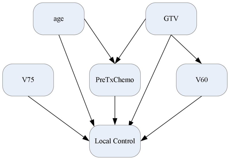
A Bayesian network constructed using the Dataset A.

4.2. Analysis of Dataset B

We also conducted experiments with the Dataset B described in Section 3.3. The Dataset B consists of physical variables and four biomarker proteins. For physical variables we used two variables (V75 and GTV) selected from our top logistic regression analysis in addition to volume regression between pre- and mid-treatment. To test the importance of each type of variables in prediction of local failure, we generated three different sub-datasets each of which consisted of physical variables, biomarker proteins, and physical variables+biomarker proteins. However, the small number of samples (n = 18) in this dataset might lead to biased estimates. As an alternative to overcome this small sample size problem, we applied the following resampling scheme. First, leave-one-out cross-validation (LOO-CV) was performed in which at each iteration, one out of the 18 available samples was reserved for testing, while using resampling with replacement from the remaining 17 samples, 2 × (n − 1) bootstrap samples (b = 34) were randomly generated for training. Note that the testing sample was not included in the new 34 training samples. Then, with these resulting testing and training sets, the same method described in Section 4.1 was repeated. Finally, we iterated this procedure 20 times and averaged the results as previously.

As can be seen in Table 3, when both physical variables and biological proteins were used, a slightly better performance (with a classification accuracy of 87.78%, r = 0.7396, rs = 0.7512, and AUC = 0.9527) was obtained compared to an accuracy of 86.11%, r = 0.7042, rs = 0.7168, and AUC = 0.9497 and an accuracy of 85.00%, r = 0.6933, rs = 0.6946, and AUC = 0.9457 with biomarker proteins and physical variables alone, respectively. From these results, it is implied that the contribution of biomarker proteins in classification of this dataset is considerable. To estimate the importance of each protein, we carried out the same experiments with only three proteins included in the network (excluding one protein at a time). Interestingly, we found that when OPN was removed, the performance was least degraded, suggesting that the contribution of OPN is relatively small compared to inflammatory cytokines in this case.

Table 3.

Performance measurements obtained using the Dataset B with different kinds of variables.

Variables\Measurement	acc	r	rs	AUC
All variables	0.8778 (0.0777)	0.7396	0.7512	0.9527
Biomarker proteins	0.8611 (0.0878)	0.7042	0.7168	0.9497
Physical variables	0.8500 (0.0457)	0.6933	0.6946	0.9457

Figure 7 shows the acceptance rate of MCMC simulation including the burn-in period of 1,000 runs. It is interesting to note that the acceptance rate quickly converged in this case. Figure 8 illustrates a Bayesian network structure with the high-confidence dependency to predict the local failure in lung cancer using heterogeneous variables. From this figure, it is observed that overall the physical variables affect protein expressions as would be expected. Figure 9 displays a Bayesian network structure built using biomarker proteins only. As shown in this figure, ACE points to TGF-β and OPN, which interestingly agrees with the signalling model assumed in the case of radiation-induced lung injury summarized by Fleckenstein et al (2007).

Figure 7.

MCMC simulation with 1,000 burn-in runs using the Dataset B.

Figure 8.

A Bayesian network constructed using combined biomarker proteins and physical variables in Dataset B.

Figure 9.

A Bayesian network constructed using biomarker proteins in Dataset B.

4.3. Evaluation of strategy effects on Bayesian structure learning algorithm

Our Bayesian structure learning algorithm was designed based on MCMC and K2 algorithms, in which the MCMC algorithm is used to obtain a node ordering that is fed as an input into the K2 algorithm. This idea was driven by the fact that the K2 algorithm is well known as a good Bayesian structure learning method in case where the node ordering is given. To test the role of K2 algorithm, we excluded it from the process and results are summarized in Table 4. That is, the table shows the results when Step 5 in Table 1 was not used, where the DAG is obtained by the directed maximum spanning tree algorithm only. For all cases, the performance was degraded considerably (particulary, when biomarker proteins were used) compared to that of the proposed method (an accuracy of 80.18%, r=0.5818, rs=0.5811, and AUC = 0.8201 using Dataset A, and an accuracy of 87.78%, r=0.7396, rs=0.7512, and AUC = 0.9527 using all variables in Dataset B).

Table 4.

Performance measurements obtained without using K2 algorithm.

Dataset\Measurement		acc	r	rc	AUC
	Dataset A	0.7679 (0.0406)	0.5077	0.5033	0.8039
	All variables	0.7778 (0.1171)	0.5409	0.5447	0.8703
Dataset B	Biomarker proteins	0.7222 (0.0980)	0.4524	0.4293	0.8383
	Physical variables	0.8333 (0.0786)	0.6737	0.6650	0.9354

In addition, to evaluate the effect of using the collective information from MCMC simulation, we tested the proposed method using the last model (Bayesian structure) after the completion of MCMC simulation. Table 5 displays the experimental results when Step 3 through 5 in Table 1 were excluded and the last model after MCMC simulation was used. Again, it is observed that the performance in all cases was somewhat degraded against the proposed method, but better than that shown in Table 4. Note that when biomarker proteins were used, the degradation of the performance is negligible. This suggests that the model after MCMC simulation is very reliable, which can be confirmed from Fig. 7 where the acceptance rate converges very quickly. The Bayesian classifier is based on probability to decide the class label of a test sample. To do that, we used Eq. (7), that is, a test sample is assigned to a class label that has probability more than 50% in binary problems. Changing the decision threshold (τ) from 0 to 1 (assigning a test sample to the control group if p(control group|X₁, X₂, ···, X_n) > τ), we generated ROC curves. The ROC curve is a useful tool to measure the discriminative value between two diagnostic groups, plotting the true positive rate (TPR) against false positive rate (FPR). Figure 10 displays ROC curves for the proposed method, the last model after the MCMC simulation, and the method without K2 algorithm using Dataset B.

Table 5.

Performance measurements obtained using the last model after the completion of MCMC simulation.

Dataset\Measurement		acc	r	rc	AUC
	Dataset A	0.7652 (0.0297)	0.4996	0.4967	0.8054
	All variables	0.8389 (0.1184)	0.6693	0.6680	0.9311
Dataset B	Biomarker proteins	0.8556 (0.0836)	0.7106	0.7110	0.9427
	Physical variables	0.8389 (0.0715)	0.6730	0.6684	0.9327

Figure 10.

Comparison of ROC curves for the proposed method, the last model after the MCMC simulation, and the method without K2 algorithm using Dataset B.

4.4. Evaluation of Bayesian structure across different datasets

To analyze dataset effect, we used Dataset B for testing, and evaluated the Bayesian structure learned from Dataset A. It is noticed that when all five variables mentioned in Section 3.2 were used, the following performance was achieved: an accuracy of 61.11%, r = 0.2039, rs = 0.2510, and AUC = 0.6062. However, when only GTV and PreTxChemo variables were selected, much better performance was attained: an accuracy of 77.78%, r = 0.5534, rs = 0.2854, and AUC = 0.6500. These results may suggest that variable selection across different datasets may play a critical role in deciding optimal performance.

5. Discussion

In this work, we investigated a Bayesian network approach for building predictive models of tumor local failure post-radiotherapy in locally advanced NSCLC patients. The proposed methods for Bayesian structure learning and classification of local failure performed relatively well when applied to the larger retrospective and the smaller prospective datasets. Our Bayesian structure learning algorithm was designed based on MCMC and K2 algorithms. We have shown that this combination is important to achieve good structure learning of the Bayesian network. The detailed network in this case with variable ranges and conditional probability tables is given in Fig. 11 for reference. When using one dataset for training and the other one for testing, the role of pre-treatment chemo seems to emerge as a more relevant variable. In our experiments, the Bayesian network based on biomarkers only seemed to provide a better performance than using physical variables only, and a combined model had slight performance improvement overall. Although the datasets we have used were relatively small and insufficient to deduce rigorous clinical or biological cause-effect relations, it is interesting to note that the Bayesian network showed interesting trends that agreed with existing knowledge in several cases. Other conflicting issues would require further analysis to understand the nature of interactions. Nevertheless, we believe that the presented methodology in this paper would be even of greater value once such data is made available.

Figure 11.

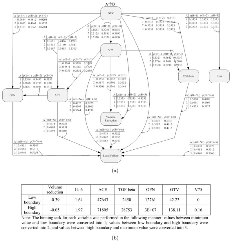
(a) A Bayesian network with probability tables for combined biomarker proteins and physical variables in Dataset B. (b) The binning boundaries for each variable.

6. Conclusions

We proposed a novel Bayesian structure learning method for modeling local failure in NSCLC patients after radiotherapy. The proposed approach was tested with two different datasets. We demonstrated that the proposed method has the potential to improve the prediction power of tumor local failure. We also showed that the Bayesian network can be used as a useful tool for identification of interactions among heterogeneous variables. Our experimental results indicate that the integration of heterogeneous variables can increase the prediction power of tumor response with higher contribution from biomarkers. However, evaluation on larger datasets is necessary to elucidate these observations.

References

- 1.Abramyuk A, Tokalov S, Zöphel K, Koch A, Szluha Lazanyi K, Gillham C, Herrmann T, Abolmaali N. Is pre-therapeutical FDG-PET/CT capable to detect high risk tumor subvolumes responsible for local failure in non-small cell lung cancer? Radiother Oncol. 2009;91:399–404. doi: 10.1016/j.radonc.2009.01.003. [DOI] [PubMed] [Google Scholar]
- 2.American Cancer Society. Cancer Facts and Figures. Atlanta, GA: American Cancer Society; 2008. [Google Scholar]
- 3.Armañanzas R, Inza I, Larrañaga P. Detecting reliable gene interactions by a hierarchy of Bayesian network classifiers. Comput Methods Progr Biomed. 2008;91:110–21. doi: 10.1016/j.cmpb.2008.02.010. [DOI] [PubMed] [Google Scholar]
- 4.Armstrong JG, Zelefsky MJ, Leibel SA, Burman C, Han C, Harrison LB, Kutcher GJ, Fuks ZY. Strategy for dose escalation using 3-dimensional conformal radiation therapy for lung cancer. Ann Oncol. 1995;6:693–7. doi: 10.1093/oxfordjournals.annonc.a059286. [DOI] [PubMed] [Google Scholar]
- 5.Chen X, Anantha G, Wang X. An effective structure learning method for constructing gene networks. Bioinformatics. 2006;22:1367–74. doi: 10.1093/bioinformatics/btl090. [DOI] [PubMed] [Google Scholar]
- 6.Choy H, et al. Phase II multicenter study of induction chemotherapy followed by concurrent efaproxiral (RSR13) and thoracic radiotherapy for patients with locally advanced non-small-cell lung cancer. J Clin Oncol. 2005;23:5918–28. doi: 10.1200/JCO.2005.08.011. [DOI] [PubMed] [Google Scholar]
- 7.Cooper G, Herskovits E. A Bayesian method for the induction of probabilistic networks from data. Mach Learn. 1992;7:309–47. [Google Scholar]
- 8.Chu YJ, Liu TH. On the shortest arborescence of a directed graph. Science Sinica. 1965;14:1396–400. [Google Scholar]
- 9.Deasy JO, Niemierko A, Herbert D, Yan D, Jackson A, Haken RT, Langer M, Sapareto S AAPM/NIH. Methodological issues in radiation dose-volume outcome analyses: summary of a joint aapm/nih workshop. Med Phys. 2002;29:2109–27. doi: 10.1118/1.1501473. [DOI] [PubMed] [Google Scholar]
- 10.Deasy JO, Blanco AH, Clark VH. CERR: a computational environment for radiotherapy research. Med Phys. 2003;30:979–85. doi: 10.1118/1.1568978. [DOI] [PubMed] [Google Scholar]
- 11.Edmonds J. Optimum branchings. J Res Nat Bur Standards. 1967;71B:233–40. [Google Scholar]
- 12.El Naqa I, Bradley J, Blanco A, Lindsay P, Vicic M, Hope A, Deasy JO. Multivariable modeling of radiotherapy outcomes, including dose-volume and clinical factors. Int J Radiat Oncol Biol Phys. 2006a;64:1275–86. doi: 10.1016/j.ijrobp.2005.11.022. [DOI] [PubMed] [Google Scholar]
- 13.El Naqa I, Suneja G, Lindsay P, Hope A, Alaly J, Vicic M, Bradley J, Apte A, Deasy JO. Dose response explorer: an integrated open-source tool for exploring and modelling radiotherapy dose-volume outcome relationships. Phys Med Biol. 2006b;51:5719–35. doi: 10.1088/0031-9155/51/22/001. [DOI] [PubMed] [Google Scholar]
- 14.El Naqa I, Deasy JO, Mu Y, Huang E, Hope AJ, Lindsay PE, Apte A, Alaly J, Bradley JD. Datamining approaches for modeling tumor control probability. Acta Oncol. 2010 doi: 10.3109/02841861003649224. [DOI] [PMC free article] [PubMed] [Google Scholar]
- 15.El Naqa I, Apte A, Yang D, Noel C, Bradley J, Deasy JO. A robust approach for estimating tumor volume change during radiotherapy of lung cancer. Med Phys. 2008;35:2956. [Google Scholar]
- 16.Fleckenstein K, Gauter-Fleckenstein B, Jackson IL, Rabbani Z, Anscher M, Vujaskovic Z. Using biological markers to predict risk of radiation injury. Semin Radiat Oncol. 2007;17:89–98. doi: 10.1016/j.semradonc.2006.11.004. [DOI] [PubMed] [Google Scholar]
- 17.Friedman N, Geiger D, Goldszmidt M. Bayesian network classifiers. Mach Learn. 1997;29:131–64. [Google Scholar]
- 18.Heckerman D, Breese JS. Causal independence for probability assessment and inference using Bayesian networks. IEEE Trans Syst Man Cybern A. 1996;26:826–31. [Google Scholar]
- 19.Jayasurya K, Fung G, Yu S, Dehing-Oberije C, De Ruysscher D, Hope A, De Neve W, Lievens Y, Lambin P, Dekkera ALAJ. Comparison of Bayesian network and support vector machine models for two-year survival prediction in lung cancer patients treated with radiotherapy. Med Phys. 2010;37:1401–7. doi: 10.1118/1.3352709. [DOI] [PubMed] [Google Scholar]
- 20.Kuschner KW, Malyarenko DI, Cooke WE, Cazares LH, Semmes OJ, Tracy ER. A Bayesian network approach to feature selection in mass spectrometry data. BMC Bioinformatics. 2010;11:177. doi: 10.1186/1471-2105-11-177. [DOI] [PMC free article] [PubMed] [Google Scholar]
- 21.Le QT, et al. An evaluation of tumor oxygenation and gene expression in patients with early stage non-small cell lung cancers. Clin Cancer Res. 2006;12:1507–14. doi: 10.1158/1078-0432.CCR-05-2049. [DOI] [PubMed] [Google Scholar]
- 22.Lindsay PE, El Naqa I, Hope AJ, Vicic M, Cui J, Bradley JD, Deasy JO. Retrospective Monte Carlo dose calculations with limited beam weight information. Med Phys. 2007;34:334–46. doi: 10.1118/1.2400826. [DOI] [PubMed] [Google Scholar]
- 23.Lucas PJF. Bayesian network modelling through qualitative pattern. Artif Intell. 2005;163:233–63. [Google Scholar]
- 24.Mu Y, Hope AJ, Lindsay P, El Naqa I, Apte A, Deasy JO, Bradley JD. Statistical modeling of tumor control probability for non-small-cell lung cancer radiotherapy. Int J Radiat Oncol Biol Phys. 2008;72:S448. [Google Scholar]
- 25.Murphy K. Bayesian Network Toolbox (BNT) 2007 http://www.cs.ubc.ca/~murphyk/Software/BNT/bnt.html.
- 26.Oh JH, Apte A, Al-Lozi R, Bradley J, El Naqa I. Towards prediction of radiation pneumonitis arising from lung cancer patients using machine learning approaches. J Radiat Oncol Inform. 2009;1:30–43. [Google Scholar]
- 27.Pernkopf F, O’Leary P. Floating search algorithm for structure learning of Bayesian network classifiers. Pattern Recognit Lett. 2003;24:2839–48. doi: 10.1016/j.patcog.2012.08.007. [DOI] [PMC free article] [PubMed] [Google Scholar]
- 28.Rübe CE, Palm J, Erren M, Fleckenstein J, König J, Remberger K, Rübe C. Cytokine plasma levels: reliable predictors for radiation pneumonitis? PLoS One. 2008;3:e2898. doi: 10.1371/journal.pone.0002898. [DOI] [PMC free article] [PubMed] [Google Scholar]
- 29.Sarkar S, Boyer KL. Integration, inference, and management of spatial information using Bayesian networks: perceptual organization. IEEE Trans Pattern Anal Mach Intell. 1993;15:256–74. [Google Scholar]
- 30.Smith W, Doctor J, Meyer J, Kalet I, Philips M. A decision aid for intensity-modulated radiation-therapy plan selection in prostate cancer based on a prognostic Bayesian network and a Markov model. Artif Intell Med. 2009;46:119–30. doi: 10.1016/j.artmed.2008.12.002. [DOI] [PMC free article] [PubMed] [Google Scholar]
- 31.van Gerven MA, Taal BG, Lucas PJ. Dynamic Bayesian networks as prognostic models for clinical patient management. J Biomed Inform. 2008;41:515–29. doi: 10.1016/j.jbi.2008.01.006. [DOI] [PubMed] [Google Scholar]
- 32.Varela AS, Saez JJBL. Utility of serum activity of angiotensin-converting enzyme as a tumor marker. Oncology. 1993;50:430–5. doi: 10.1159/000227224. [DOI] [PubMed] [Google Scholar]
- 33.Velikova M, Samulski M, Lucas PJF, Karssemeijer N. Improved mammographic CAD performance using multi-view information: a Bayesian network framework. Phys Med Biol. 2009;54:1131–47. doi: 10.1088/0031-9155/54/5/003. [DOI] [PubMed] [Google Scholar]
- 34.Witten I, Frank E. Data Mining: Practical Machine Learning Tools and Techniques. 2. San Francisco: Morgan Kaufmann; 2005. [Google Scholar]