The Developmental Rules of Neural Superposition in Drosophila

Summary

Complicated neuronal circuits can be genetically encoded, but the underlying developmental algorithms remain largely unknown. Here, we describe a developmental algorithm for the specification of synaptic partner cells through axonal sorting in the Drosophila visual map. Our approach combines intravital imaging of growth cone dynamics in developing brains of intact pupae and data-driven computational modeling. These analyses suggest that three simple rules are sufficient to generate the seemingly complex neural superposition wiring of the fly visual map without an elaborate molecular matchmaking code. Our computational model explains robust and precise wiring in a crowded brain region despite extensive growth cone overlaps and provides a framework for matching molecular mechanisms with the rules they execute. Finally, ordered geometric axon terminal arrangements that are not required for neural superposition are a side product of the developmental algorithm, thus elucidating neural circuit connectivity that remained unexplained based on adult structure and function alone.

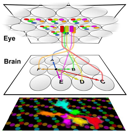
Graphical abstract

Introduction

A central question in neuroscience is how neural circuits self-organize into functional structures during development. The wiring of compound eyes to the brain of flies provides a fascinating model system for studying this question (Agi et al., 2014; Land, 2005; Meinertzhagen, 1976; Nilsson, 1989). In particular, the neural superposition eye, such as found in advanced flies, is characterized by a complicated wiring diagram (Fig. 1): each point in visual space is captured by multiple photoreceptors, each in a different ommatidium, that converge upon the same synaptic unit (cartridge) in the brain (Fig. 1B); different photoreceptors within the same ommatidium view different points in visual space and project to neighboring cartridges (Fig. 1A) (Braitenberg, 1967; Clandinin and Zipursky, 2002; Kirschfeld, 1967; Vigier, 1907a, b). The correct pooling of axon terminals that view the same point in space into a single cartridge increases sensitivity without loss of spatial resolution compared with simpler, ancestral eye types (Agi et al., 2014; Braitenberg, 1967; Kirschfeld, 1967; Nilsson, 1989). The developmental process underlying neural superposition is remarkable, because each individual axon, amongst thousands of neighboring axons in the brain, must be sorted together with those few axons that receive input from the same point in visual space.

Figure 1. The Neural Superposition Sorting Problem.

(A) The six outer photoreceptors R1–R6 from a single unit eye (ommatidium) receive input from six different points in the visual environment and project to six separate synaptic units (cartridges) in the brain. (B) The six R1–R6 photoreceptors from six different ommatidia that receive input from the same point in visual space connect to the same cartridge, in a pattern that is the reciprocal of that in (A). (C) Schematic view of a lamina section from dorsal (left) to ventral (right) across the equator. The color-coded R1–R6 axons from different ommatidia that receive input from points in the environment A–F are shown in their final cartridge arrangement on the left. The circular arrangement of axon terminals in the cartidges shows the precise rotational stereotypic arrangement of R1–R6.

A classic model of neural superposition is found in the Drosophila compound eye, which contains ~800 ommatidia. Each ommatidium projects a bundle of eight photoreceptor (retinula or R cell) axons into the brain. Six of these photoreceptors, R1–R6 (the focus of our current study) form the primary visual map in the lamina (first optic neuropil) of the fly brain (Fig. 1A; R1–R6 are color-labeled consistently throughout the paper: R1, blue; R2, green; R3, red; R4, yellow; R5, magenta, R6, orange). The R1–R6 axons from one bundle that receive input from six different points in visual space are denoted A–F (Fig. 1A–C).

After neural superposition is established, the R cells have a precise organization of the six subtypes around the circumference of cartridges, R1 neighbors R2, which neighbors R3, etc., referred to as “rotational stereotypy” (Fig. 1B, C). The precision of rotational stereotypy is noteworthy, as the six axon terminals in a cartridge carry the same input information and synapse with the same postsynaptic target cells (Braitenberg, 1967; Trujillo-Cenóz, 1965). Hence, rotational stereotypy is not a functional requirement for neural superposition, and increases the demands placed upon the sorting problem from 800 cartridges to 4800 (800 × 6 R1–R6) precise terminal positions. The role, development and evolutionary origin of this wiring precision are unknown.

The neural superposition wiring diagram has a “canonical” pattern of six R-cell axon terminals per cartridge. An equator from anterior to posterior divides the compound eye as well as the wiring pattern in the lamina into dorsal and ventral halves. The wiring patterns in each half of the lamina are mirror-symmetric to one another with respect to the equator axis (blue line in Fig. 1C). As a consequence, six rows of “non-canonical” cartridges exist at the equator that contain stereotypic compositions of seven or eight R1–R6-cell axon terminals (Fig. 1C) (Horridge and Meinertzhagen, 1970; Meinertzhagen and Hanson, 1993). The three different types of equator cartridges also exhibit rotational stereotypy, albeit of three distinct types (Fig. 1C) that remain functionally unexplained (Horridge and Meinertzhagen, 1970). It is unclear what common developmental rules or mechanisms might robustly encode the canonical as well as the three types of equator cartridges (Fig. 1C).

The Drosophila visual system is an example for a genetically encoded neural circuit in which a developmental sorting step precedes and ensures synaptic specificity between input neurons and their targets (Hiesinger et al., 2006). Many aspects of the developmental sorting step have been characterized in detail, including the formation of an initial grid by lamina cells (Hadjieconomou et al., 2011; Meinertzhagen and Hanson, 1993). Previous studies suggested the possibility of simple developmental rules underlying this sorting process (Clandinin and Zipursky, 2000; Meinertzhagen, 1972; Meinertzhagen and Hanson, 1993). Furthermore, work in recent years has revealed molecular mechanistic insight into how differential adhesion of guidance receptors may play a key role in growth cone sorting (Chen and Clandinin, 2008; Schwabe et al., 2013). However, no rule set or algorithm has been formulated that is sufficient to generate precise neural superposition and equator wiring. Two key challenges have been: (1) the inability to monitor the dynamic sorting process live in developing flies; and (2) lack of quantitative, data-driven models to conceptualize or test our understanding of this apparently complicated process.

Here, we report live imaging of R1–R6 growth cone dynamics in intact, developing pupa and the derivation of a model that summarizes our conceptual understanding of the development of neural superposition. We propose that three simple rules are sufficient to provide a solution to the neural superposition sorting problem. Systematic tests of these rules in a computational model reveal that the same rule set leads to precise superposition and the three types of cartridges observed at the equator.

Results

Intravital imaging reveals the morphogenesis of the lamina during brain development

In order to visualize the growth cone movements that establish neural superposition, we made use of multiphoton time-lapse microscopy to image through the eye of intact developing pupae (intravital imaging; Fig. 2A). This approach allowed us to visualize both large-scale tissue movements as well as small-scale growth cone dynamics in the developing pupa. Importantly, our method is non-invasive, and only data from pupae that completed development normally were used throughout this study.

Figure 2. Intravital imaging reveals the morphogenesis of the lamina and photoreceptor growth cones during brain development.

(A) Imaging chamber for 2-photon live imaging through the intact, developing pupal eye. Right panel: side view of all photoreceptors labeled with membrane tagged CD4-tdGFP at 20h APF. (B–D) View of the same specimen as in (A) from inside the brain (B), with the axons viewed from a cut plane between eye and lamina (C) and after 20h hours of further development (D).

(E–G) Side view of the same specimen as in (A–D) in 10h developmental intervals. See also Movie 01.

(H–J) Side views of a specimen at the indicated time points with sparse photoreceptor labeling and individual identified growth cones marked in R1–R6-specific colors as defined in Figure 1.

(K–L) Visualization of individually segmented growth cones from the specimen shown in (H–J) at 25h APF (K) and 40h APF (L).

The lamina plexus is a temporary structure in which R1–R6 growth cones sort in a two-dimensional, dynamically warping plane (Meinertzhagen and Hanson, 1993). Labeling of all photoreceptors with a membrane-tagged CD4-tdGFP (Han et al., 2011) throughout the time period of neural superposition development from 20–40h after puparium formation (APF) allowed the visualization of R1–R6 projections that form the lamina plexus in relation to the deeper projections of R7/8 axons (Fig. 2A–D).

Our intravital imaging technique enabled us to identify two major large-scale tissue movements that were, to our knowledge, previously uncharacterized (Figure 2A, Movie 1). First, we observed a 90° rotation of the entire lamina-medulla complex (Fig. 2B–D). Second, the lamina plexus flattens in a temporal wave of shortening axons underneath the eye (Fig. 2E–G). The 20–40h temporal wave alters the orientation of the lamina from a plane close to perpendicular to one that is parallel with both the eye and the medulla (Fig. 2E–G; red arrows in Fig. 2F). Hence, the relative change of angles between the lamina plexus and medulla known as “medulla rotation” (Meinertzhagen and Hanson, 1993; White and Kankel, 1978) results from the progressive intercalation of the lamina plexus between the eye and medulla. This developmental process ensures a perfect alignment of eye and lamina with minimal axon length for the transmission of graded potentials. Our understanding of lamina plexus movements allowed us to distinguish individual growth cone dynamics from movements of the tissue in which they are embedded.

To visualize individual growth cones in the lamina plexus we utilized a sparse labeling technique (Experimental Procedures, (Rintelen et al., 2001)). At 40h APF, all randomly labeled growth cones fall into one of six distinct classes based on their three-dimensional morphology and orientation. Tracing axons back to their unique cell body positions in the eye unequivocally identified each as an R1–R6 subtype (color-coded as in Figure 1) (Fig. 2H–J). Next, we followed each growth cone through all time points back to 25h APF (Fig. 2K, L; Movie 2). As the warped plane of the lamina plexus unfolds, different parts change their position relative to the fixed light path during intravital imaging. We therefore corrected clusters of 2–12 growth cones for these tissue movements (Experimental Procedures). The resulting data provide complete four-dimensional dynamics of identified R1–R6 growth cones throughout the process of superposition sorting in a two-dimensional plane.

The Scaffolding Rule: bipolar growth cone “heels” generate a stable framework for the sorting process

During the establishment of neural superposition, six times 800 growth cones leave their origination bundles and terminate in surrounding destination cartridges (Fig. 1A). This sorting of axons predicts the repositioning of neighboring growth cones relative to each other. Such rearrangements of individual growth cones were inferred from previous studies on fixed preparations at timed stages (Meinertzhagen and Hanson, 1993; Trujillo-Cenóz and Melamed, 1973) and should be readily apparent in our intravital imaging data.

Surprisingly, we did not observe the expected rearrangements of growth cones between 25–40h APF, despite the emergence of polarized, extended growth cone shapes. Four out of the six subtypes develop distinct bipolar growth cone shapes that were not previously described in fixed preparations. After 30h APF we observed for R1, R3, R4 and R6 distinct ‘heel’ structures anchored at the original arrival points of the axons (arrowheads in Fig. 3A–F) and distinct ‘front’ densities in the direction of polar extension (arrows in Fig. 3D–F). A time-lapse movie of the growth cone heels revealed no rearrangements of their relative positions (Fig. 3A′–F′; Movie 3). In contrast, the growth cone fronts progressively move away from their respective heels with subtype-specific speeds and angles. Distinct filopodial movements are clearly visible at both the heels (arrowheads) and fronts (arrows) (Fig. 3A–F). Importantly, bipolarity gives the two active ends of each growth cone—the stationary heel and the extending front—the potential to execute different functions during growth cone sorting.

Figure 3. The Scaffolding Rule: bipolar growth cones generate a stable framework that facilitates the sorting problem.

(A–F) Movements of a cluster of 12 growth cones between 25h and 40h APF. Arrowheads denote heels, arrows mark growth cone fronts. (A′-F′) show the positions of the heels only. Note that the lower part of this cluster expands due to lamina unfolding between 25–34h APF, yet no heels shift relative to each other. Scale bar: 5μm. See Movies 02 and 03.

(G–I) Cross-section through the lamina plexus at 40h APF for the same specimen as shown in (A–F). (G) Background labeling reveals a rhomboidal 80°/100° grid in the lamina plexus that overlaps all growth cone fronts (ovals). In contrast, all heels (arrows) are located outside the grid defined by R-cell fronts. Scale bar: 5μm. (H) Extrapolation of the position of all heels in the scaffold. (I) Vectors of R1–R6 growth cones at 40h APF based on measurements at 40h APF.

(J) Updated schematic of growth cone sorting in the lamina plexus, viewed from the eye, based on the schematics shown in Figs. 1C,D. Note that the heels have a horseshoe-shaped arrangement within the circular ‘arrival units’ shown in Fig. 1C, whereas the target ovals form a intercalated grid.

(K) Cartridge distances in the lamina plexus between 20h and 40h APF reveal scaffold stability throughout growth cone sorting. Measurements were taken from fixed preparations shown in Fig. S1. Data shown: mean +/− SD (n is ≥67 for each time point).

Fortuitously, our imaging data revealed a background grid-like pattern (Fig. 3G). None of the identified growth cone heels, but all fronts, overlap with this background pattern. Hence, the visible pattern in the live imaging data of sparsely labeled growth cones coincides with the growth cone fronts in the target area, while all growth cone heels are positioned around these regions. Based on these data, we extrapolated the positions of heels and fronts for all R-cells (Fig. 3H). The heels occupy about half of the space in the two-dimensional grid and provide a complementary pattern to the growth cone fronts (Fig. 3H). The heel and target grid frame the starting and ending positions of growth cone sorting in 2D (Fig. 3J)

The Extension Rule: Quantitative analysis of growth cone dynamics reveals synchronized extension programs specific for each R1–R6 subtype

We next analyzed the dynamics of growth cone extension between 25h and 40h APF. For each time point and each of the 58 growth cones, we measured the position of the: (1) heel (solid circle), (2) front (open circle), (3) tip of the longest filopodium extending away from the heel (small solid circle), and (4) tip of the longest filopodium extending away from the front (small open circle) (Fig. 4A; Movie 5). Heel-Front separation became apparent at distinct time points for different R1–R6 subtypes (asterisks in Fig. 4B). The distances between fronts and heels increase steadily during subtype-specific 5–10 hour time windows (black lines in Fig. 4B, see also Fig. 4G–I for traces of individual cells): R3 and R4 extend for more than 10 hours from 25h APF onwards; R1 and R6 extend between 30h and 37h APF; and R2 and R5 show minimal extension between 30h and 35h APF. Thus, polarized growth of a directed collateral, as previously speculated (Trujillo-Cenóz and Melamed, 1973) is not supported from our observations.

Figure 4. The Extension Rule: Quantitative analysis of growth cone dynamics reveals synchronized extension programs specific for each R1–R6 subtype.

(A) Schematic of quantified heel, front and filopodial positions (same specimen as Fig. 3). (B) Heel-Front distance for R1–R6 between 25h–40h APF. Asterisks: denote the subtype-specific initiation of extension and black lines highlight periods of near-linear extension. (C) Heel-Front angles between 25h–40h APF reveals angle constancy for R1–R6 throughout the sorting process. (D) Angles between heel and longest front filopodium reveal average filopodial explorations at closely matching angles. (E–F) Angles of the longest front and heel filopodial exploration. (G–I) Extension dynamics are identical across the A–P axis, indicating synchronous movements across the entire lamina plexus. See also Fig. S2. (B–G) Data shown: mean +/− SD.

All six growth cone subtypes additionally exhibit angular constancy over the entire time period of their extension (Fig. 4C). Next, we analyzed the angles between heels and the tips of the longest front filopodia, which are unequivocal and objective points for each growth cone and time point. The average of the longest front filopodia for all growth cones of one subtype revealed the same angular constancy and the same angles over time as those determined by manual front identification (compare Fig. 4C, D). We noted that filopodia at the heel and front revealed different dynamics with characteristic filopodial exploration angles (Fig. 4E, F) and subtype-specific lengths of exploration (Fig. S2A–C). In contrast to the polarized front filopodia (Fig. 4E), all R1–R6 heel filopodia randomly explored angles around and away from the direction of polarity (Fig. 4F). This observation further supports the notion of different functions of growth cone heels and fronts.

As shown above (Fig. 2B–G), the entire lamina plexus undergoes a progressive alignment in an anterior to posterior temporal wave of shortening axons that occurs between 20–40h APF, which is concurrent with growth cone sorting in the lamina plexus. We sought to determine whether growth cone dynamics follow this temporal wave by analyzing growth cones in different positions along the anterior to posterior axis (i.e. in different parts of the unfolding two-dimensional array, and consequently for axon bundles of different ages). We found that growth cones of the same subtypes at different positions along the anterior to posterior axis exhibit no significant differences, neither in their start time nor their extension behavior (Fig. 4G–I). These measurements are consistent with previous observations in fixed preparations that suggested growth cones of distinct subtypes exhibit no morphological gradient (Hiesinger et al., 2006; Schwabe et al., 2013). We conclude that the tissue movements of the lamina between 20–40h APF are unlikely to play an instructive role in the synchronous sorting of growth cones.

A previous study on fixed preparations proposed that the development of polarity as early as 20h APF precedes and predicts the direction of a separate extension phase after 32h APF (Schwabe et al., 2013). However, our live imaging did not reveal separate polarization and extension phases at least for time points after 25h APF, but rather showed one continuous extension process. The angles and speeds specific to each R1–R6 subtype ensure that all R-cell growth cone fronts ‘meet’ in the correct target areas for neural superposition as defined by the corresponding heel scaffold. A key aspect of this ‘extension rule’ is that all growth cones of each of the six R-cell subtypes exhibit identical extension behavior across the entire lamina, including the equator region (see below).

The Stop Rule - Part 1: Growth cone fronts overlap with multiple targets in the scaffold

How does growth cone extension stop? We systematically considered extension stop rules ranging from stop rules that require no interactions with surrounding cells, to stop rules that integrate multiple intercellular interactions. We envision that ‘no interaction’ stop rules would be either: (1) ‘programmed’ into cell-autonomous extension, or (2) triggered by an exogenous stop signal that functions synchronously across the entire lamina plexus. In both cases the targeting accuracy depends fully on the precision of the scaffold and the extension angles. Our imaging data show that the scaffold within the unfolding lamina exhibits minor warped or bent areas (Fig. S1) and that the measured extension angles have standard deviations of around 10° (Fig. 4C). A lack of feedback from the target area for either of the ‘no interaction’ stop rules would thereby lead to inaccuracies in arrival points of growth cone fronts. This would likely lead to high error rates for wiring and especially rotational stereotypy, which has not been observed (see discussion in section Validation at the Equator below). We therefore consider ‘no interaction’ stop rules unlikely, though they remain theoretical possibilities. In the following, we focus on interaction-based stop rules, but return to a test of both types of rules in the last section.

Arguably the simplest interaction-based stop rule would be the recognition of a target cell. Can a target cell be robustly recognized amongst incorrect alternatives in the densely packed lamina plexus? The main cells in the putative target region are the lamina neurons, or L-cells, which also are R1–R6’s prospective synaptic targets (Fig. S1). Throughout the establishment of neural superposition the L-cells are positioned in the correct target areas and surrounded by R heels (Fig. 5A; Fig. S1). However, the extent and arrangement of L-cell processes between 20h–35h APF also pose a potential problem for L-cells to provide restricted target cues. At 28h APF, L-cell processes form a filopodial mesh that covers most of the lamina plexus (Fig. 5A). This network of L-cell processes overlaps to a large extent with the R1–R6 growth cones. For example, R3 growth cones overlap to different degrees with three to six L-cell clusters in potential target areas. Importantly, the closest target areas to the R3 growth cones are incorrect (Fig. 5B, black asterisks).

Figure 5. The Stop Rule - Part 1: How good a target is the target?

(A) Single frame at 28h APF from a 20h time-lapse movie of all target L-cells. Arrow: single representative heel bundle (arrival unit). The boxed area marks the heel scaffold and the blue line marks the equator. Scale bar: 5μm. (B) Enlarged region within the box in (A) with one heel bundle shown. The shape of a representative R3 originating from this heel bundle reveals overlap with at least two incorrect targets (black asterisks) in addition to the correct target (white asterisk). (C) Reference schematic for quantifications and the computational model; see text for details. (D–F) Analysis of target recognition with different sensing radii for an R-cell front in a schematic (D), a single representative R3 growth cone (E), and an overlay of all R3 growth cones analyzed for this study. (G–L) Overlap with any target throughout the simulated move of three R-cell sensing fronts of differing radii. Arrows indicate partial overlap, arrowheads indicate premature final stops. See also Fig. S3.

To analyze quantitatively the conditions under which L-cells could serve as targets, we developed a computational model. The scaffolding rule was implemented using the measured heel grid (Fig. 3J). The extension rule was implemented using synchronous movements of R front sensing areas (Fig. 4). We defined the distance between centers of adjacent target areas as D=1 (5.5 μm; Fig. 5C; Fig. S3). However, the shape and area of R-cell growth cone fronts that sense potential targets are not easily determined from the biological data. Here, we approximated sensing regions of R cell fronts as discs. (Such a sensing region can be viewed as isotropic or anisotropic depending on whether the sensing disc is conceptualized as being centered at—or extended ahead of—the growth cone front.) Our data suggests a range of sensing radii (SRs) between 0.22 and 0.5: an area defined by SR=0.22 is contained in >90% of the imaged R front areas; SR=0.36 is contained in 60–90% of R front areas; and SR=0.5 (a circle with a full cartridge diameter) is contained in >30% of imaged R front areas.

If minimal overlap of an R-cell front with a single target region were sufficient to stop growth cone extension, even a relatively small sensing radius would lead to incorrect targeting (black arrow in Fig. 5D). However, R3 fronts experience partial overlap in passing with even relatively small incorrect targets (Fig. 5D–F, gray circles with SR = 0.22) (Fig. 5D). (This would also be true for an elliptic R-cell front shape—either centered at or extended ahead of the growth cone front—that has a much larger SR in the direction of polarity; see blue shapes at 30h and 35h time points in Fig. 5D). Partial overlap is apparent in the case of a single representative growth cone over time (Fig. 5E) and especially for outlines of all imaged R3 growth cones (Fig. 5F). This observation suggests that partial overlap must be permissible to avoid stopping the R3 fronts prematurely. Therefore, in our model we allowed R fronts to ignore partial overlaps with targets, up to the distance SR, during extension. For example, the partial overlaps highlighted by the black arrow in Figs. 5D, G, J are not sufficient to arrest R3 growth cone extension, because the distance between the overlapping circumferences is less than SR=0.22. Hence, the model allowed us to systematically explore stop rules based on varying R-cell front sizes and overlaps with targets.

We first simulated the extension of R-cell growth cone fronts away from the heels in the scaffold with measured angles (see Suppl. Exp. Proc.). Our simulation shows that correct sorting is possible for R-cell fronts and target sensing areas as small as SR=0.22. The total overlap with any target for each R-cell front with SR=0.22 (moving at measured angles) reveals overlap of R3 with an incorrect target (arrows in Fig. 5D, G), although the overlap is below threshold for stopping. Note that this threshold is not an arbitrarily fixed value, because testing different SRs includes tests for different permissible amounts of overlap (Fig. 5L). For an R3 front with SR=0.36 this overlap reaches SR and causes an early, incorrect stop (arrowhead in Fig. 5H); R fronts with SR=0.5 exhibit so much target overlap with surrounding targets that none of them move far (Fig. 5I).

Finally, we tested whether possible measurement inaccuracies caused this lack of robustness, by simulating targeting with ideal (mathematically computed) angles from heel to target regions (Fig. 5D, J, K). Remarkably, the ideal model yielded almost identical results to measured data, including a failure to establish neural superposition wiring with growth cone front SRs of 0.36 and above (arrowhead in Fig. 5K).

Our analyses of a ‘target only’ stop rule indicate that L-cells—or any other cue at the target area—can function as a stop signal only within substantial constraints. Specifically, our model shows that the premature arrest of growth cone extension can be averted only if R-cell fronts use a sensing area that is either insensitive to or much smaller than the apparent morphological area covered by the growth cone front and its filopodia when it passes the incorrect targets.

The Stop Rule - Part 2: Overlaps between R1–R6 growth cone fronts can increase the robustness of the stop rule

In addition to overlaps of R1–R6 fronts with multiple target areas, overlaps amongst the R1–R6 fronts themselves in the correct target region are already apparent around 25h APF (Fig. 6A–C). This overlap increases substantially until 35h APF (Fig. 6D–F). At the end of growth cone sorting, each R1–R6 front covers ~50% or more of its target area, which is shared with the five other growth cone fronts needed to establish correct neural superposition (Fig. 6G; arrow shows overlap of all six ‘incoming’ R-cell fronts needed to establish the correct pattern of sorting). We therefore incorporated increasing overlaps between R1–R6 fronts into the model.

Figure 6. The Stop Rule - Part 2: R1–R6 growth cone front overlaps can increase the robustness of the stop rule.

(A–F) R1–R6 outlines from intravital imaging data for 25h APF (A–C) and 35h APF (D–F). The outlines are shown in subtype pairs for R1+R3 (A, D), R2+R5 (B, E) and R4+R6) (C, F) to highlight the amount and increase in overlap in the target area (dark ovals) during these 10 hours of growth cone extension. (G) Representative growth cones at 40h APF. Shown are the ‘outgoing’ growth cones from one bundle, the ‘incoming’ growth cones to one target (arrow) and a pair or R1+R3 to highlight covering and overlap in the target area.

(H) Computer simulations with a stop rule using coincidence detection of the target plus all other R fronts and the sensing radii 0.36 and 0.5. (I) R1–R6 front overlaps with other R-cell fronts or targets with the noted sensing radii. (J) Systematic parameter scan of all combinatorial stop rules and sensing areas from SR=0.2–0.5. (K–M) Systematic scans for sensing radii 0–0.5, sensing start time 20–40h and +/−10° randomly varied extension angles are shown for the ‘target only’ rule and two combinatorial stop rules without (L) and with target (M). Each data point was simulated 100 times for angles that were randomly offset +/−10° (Fig. S4).

We first simulated a ‘combinatorial overlap + target’ stop rule, in which an R-cell growth cone front stops only if it encounters a target area plus five other R-cell fronts (defined by overlap of a given SR). In order to allow the R-cell fronts to move out of their originating bundles, the stop rule was required to begin shortly after extension starts (Experimental Procedures). A simulation with SR=0.36, which failed using the ‘target only’ stop rule (Fig. 5D, H), reveals correct establishment of neural superposition wiring in the model (Fig. 6H, top row) (Movie 6 shows a ‘combinatorial overlap’ simulation without requiring a target, which behaves identically to the ‘combinatorial overlap + target’ stop rule, see below). Remarkably, even an extraordinarily large sensing area, with a diameter of the entire inter-cartridge distance (using SR=0.5), can correctly establish neural superposition (Movie 6; Fig. 6H bottom row). This is surprising because larger sensing radii have a higher chance to cause a premature stop due to overlap. However, R fronts exhibit a collective, sharp increase of total area overlap with other R fronts and target areas only once they reach the correct target area (Fig. 6I).

Next, we systematically compared the precision of wiring for ‘combinatorial overlap + target’ stop rules for different numbers k (k = 0 to 5) of other R-cell fronts. We additionally performed this test while scanning SR from 0.2 to 0.5. Our results show that all combinatorial stop rules for overlap with k ≥ 3 other R cells perform more robustly with larger sensing areas than the ‘target only’ (k = 0) rule (Fig. 6J). Stop rules that combine target recognition with the sensing of 4 or 5 other R-cell fronts function robustly over the wide range of scanned sensing radii. Hence, these findings suggest that R fronts of large sizes and substantial overlap can target correctly if the target is defined by coincidence detection of the target plus other R-cell fronts, independent of their subtype.

Surprisingly, a ‘combinatorial overlap’ stop rule, based on R-cell front sensing when the target area itself does not contribute to the combinatorial stop rule, functions robustly (Movie 6). Specifically, recognition of k ≥ 4 other R-cell fronts without the target area itself is nearly as robust as when the target area is included (Fig. 6J). This finding reveals the theoretical possibility that target recognition during growth cone sorting may be an intrinsic property of the R-cell growth cone array, and does not require the recognition of the actual target itself (e.g. L-cells) as part of the stop rule. In addition, our results show that even in an unconstrained model where all R cells sense all other R cells, the geometry of the scaffold ensures that only the “right” R cell fronts stop each other in the right place (Movie 6).

Next, we quantitatively assessed the robustness of the ‘target only’ and ‘combinatorial overlap’ models with respect to perturbations in extension angle. We computed the probability of accurate neural superposition patterning in the case when the extension direction of each R1–R6 subtype was randomly varied up to +/−10 degrees around its idealized direction (Fig. S4, n = 100 simulations per condition). We created phase plane diagrams of accuracy as a function of the sensing radii of R-cell fronts, sensing start time and stop rules (Fig. 6K–M). The simulations of the ‘target only’ model reveal that correct neural superposition wiring is only robust for small sensing radii (SR<0.25) if the overlap is sensed throughout sorting (sensing start time earlier than 30h APF, Fig. 6K). However, larger sensing radii can function robustly in the ‘target only’ model only if overlap sensing is turned on at 35h APF or later, i.e. at the very end of extension, after R-cell fronts have already passed incorrect targets. Such a late overlap sensing start would be facilitated by the synchronous nature of growth cone sorting. However, the ‘target only’ model lacks robustness for sensing radii that match the morphological appearance of the imaged R fronts (Fig, 5D–F; Fig. 6A–G; Fig. S4A) and overlap sensing prior to 32h APF. In contrast, ‘combinatorial overlap’ stop rules based on R-cell front sensing (with or without the target) exhibit robustness for larger sensing radii that have extensive R-cell overlap throughout sorting. Consistent with the biologically relevant parameters of SR>0.2 and the time for actual sorting to fall between 20h and 40h APF (red boxes in Fig. 6K–M), these combinatorial stop rules exhibit a high probability of perfect wiring (yellow) for SR>0.3 despite the random angle variation (Fig. S4B, C). In summary, our model indicates that ‘combinatorial overlap’ stop rules that utilize R-cell front overlaps, as observed in the imaging data, greatly improve robustness of the stop rule. The model further predicts optimal sensing radii between 0.3 and 0.4, which closely resembles the observed size of growth cone fronts (compare Fig. 5E and Fig. 6A–G). However, our modelling results alone only reveal the ‘combinatorial overlap’ stop rule as a robust solution, but do not yet exclude the ‘target only’ or ‘no interaction’ stop rules.

Validation at the Equator: The three neural superposition rules provide an explanation for reduced equator wiring robustness and all four types of rotational stereotypy within cartridges observed in wild type

A test of the growth cone extension and stop rules in perturbation experiments by ablating R- or L-cells is not easily possible, because loss of any of the involved cell types disrupts the scaffold. However, the wiring pattern around the equator provides an important natural experiment that tests the model: six rows of cartridges have varying composition and represent three different degrees of disruption of the canonical wiring pattern (Fig. 1C; Fig. 7A). Specifically, cartridges of the three rows near the equator differ from the canonical cartridge patterning by containing: an extra R3 (wiring-type ‘7R’; Fig. 7A), an extra R3 and an extra R4 (‘8R type 1’; Fig. 7A) and extra R2, R3, R4 and R5 with missing R1 and R6 cells (wiring-type ‘8R type 2’; Fig. 7A) respectively. Each of these three equator cartridge types exhibit a distinct pattern of rotational stereotypy (Fig. 1C; Fig. 7A) (Horridge and Meinertzhagen, 1970; Meinertzhagen, 1972). This enigmatic and ‘overly precise’ wiring specificity has remained unexplained.

Figure 7. The equator and rotational stereotypy validate the developmental algorithm and indicate a role for R1–R6 overlap sensing as part of the stop rule, but not the extension rule.

(A–B) Schematic of all types of main and equator-type cartridges, their composition (top), the stereotypy of the arrangement of the varying types of R cells (A) and the result of a simulation of the developmental algorithm using the computational model (B). Simulation with SR=0.22 and a stop rule of ‘target+4R’

(C–G) Comparative analyses of R3 and R4 growth cone dynamics in the main lamina and across the equator.

(H–M) Systematic parameter scans for the labeled stop rules and all sensing radii 0.2–0.5 across the main lamina and equator. The red bar indicates at what sensing radius correct superposition sorting fails. Note that all stop rules that include R front sensing exhibit reduced equator robustness at larger sensing radii. See also Figs. S5–6.

The computational model based on a combinatorial stop rule generates precise equator wiring and all precise patterns of rotational stereotypy in the placement of R-cell terminals in cartridge profiles (Fig. 7B; Movie 7). This observation suggests that the apparent precision of the wiring pattern is a side effect of the developmental algorithm presented here. The observed four types of R-terminal rotational stereotypy also provide support for the idea that R-cell front interactions are part of the stop rule. The measured vectors (Fig. 3J) and R front overlap (Fig. 6) alone do not obviously lead to rotational stereotypy. However, recognition and ‘sandwiching’ between direct neighbors provide an elegant mechanism that preserves the rotational stereotypy, whereas it is more difficult to envision how R-cell fronts would retain the exact same two R cell subtypes as neighbors without sensing each other.

To test more directly the role of interactions between R-cell fronts during growth cone targeting, we analyzed the growth cone dynamics and robustness underlying extension and stop rules in the equator vs. main lamina. The longest growth cones (R3s) need to navigate seven different environments near the equator (red vectors in Fig. 7A). We hypothesized that if R-cell front interactions instruct either the growth cone’s extension angle or its speed, then the altered equator environments should cause altered growth cone behavior. To test this hypothesis, we compared growth cones at the equator with those in the main lamina. As shown in Fig. 7C, outlines of equator and non-equator R3s and R4s appear indistinguishable for all measured parameters and time points. Specifically, we measured Heel-Front length (Fig. 7D), Heel-Front Filopodia length (Fig. 7E), Heel-Front angle (Fig. 7F), Heel-Front Filopodia angle (Fig. 7G) as well as the lengths and angles of Heel-Heel Filopodia and Front-Front Filopodia (Fig. S5A). These measurements support the idea that R growth cones extend according to the same guiding principle in both equatorial and non-equatorial regions. However, it is difficult to envision a molecular mechanism for interactions between the R-cell fronts for the seven different environments that would lead to identical dynamics. We conclude that these measurements do not support a mechanism whereby R front-R front interactions (for R-cells originating in different bundles) instruct extension angle or speed.

Next, we asked whether R-cell front interactions might play a role as part of the stop rule, as suggested by our robustness analyses in the main lamina (Fig. 6K–M) and the observation of rotational stereotypy in all parts of the lamina (Figs. 1C, 7B). The equator region provides a decisive test, as our model predicts reduced robustness at the equator for any stop rule that involves R-cell front interactions, but not for ‘target only’ or ‘no interaction’ stop rules (comp. Fig. S5B–D and Fig. 6K–M). The ‘target only’ stop rule has the same robustness at and away from the equator, with wiring succeeding or failing at the same sensing radii (red vertical line in Fig. 7H) because the target grid is isotropic across the entire lamina (e.g. Fig. 5A).

Similarly, all ‘no interaction’ stop rules have the same robustness at or away from the equator (data not shown), because the stopping condition is independent of the R-cell environment. In contrast, all stop rules based on R front sensing exhibit reduced equator robustness compared with neural superposition wiring in the main lamina (broken red lines in Fig. 7I–M). This is consistent with the prediction that increased numbers of R-cell fronts at the equator more easily lead to a premature stop that results from an R-cell front meeting head on with other R-cell fronts. Hence, we hypothesize that if R front sensing is part of the stop rule, the wild-type equator should exhibit reduced robustness, which would be apparent as an increased wild-type error rate.

A test of this hypothesis is available in the form of two seminal single-axon tracing studies in the neural superposition eye of the blow fly Calliphora (Horridge and Meinertzhagen, 1970; Meinertzhagen, 1972). Of a combined ~1200 individually traced axons, none terminated in an incorrect neural superposition cartridge of the main lamina. In contrast, Meinertzhagen (1972) identified 17 targeting errors at a wild-type equator. All of these targeting errors represent premature stops in the correct direction, as predicted by our model. Finally, rotational stereotypy errors are more commonly observed, but again almost exclusively observed at the equator (Horridge and Meinertzhagen, 1970; Meinertzhagen, 1972). Hence, the observation of wiring errors at the wild-type equator, in conjunction with the observations that R-cell front interactions are not required during extension, supports the hypothesis that R-cell front interactions are part of the stop rule and argues against both the ‘no interaction’ and ‘target only’ stop rules. Similar to the equator, our model generates edge cartridges at the borders of the lamina that match and explain experimental observations (Meinertzhagen and Hanson, 1993) (Supplemental Materials and Fig. S6).

Discussion

Here, we describe a developmental algorithm for the axonal sorting of ~4800 presynaptic cells in the primary visual map of Drosophila. Our work suggests that the neural superposition wiring diagram found in adult fly brains can be established through simple, local pattern formation principles without the need for an elaborate molecular matchmaking code. Our codification of the developmental algorithm reveals quantitative constraints and provides a conceptual framework for molecular mechanisms that execute these rules.

Three Rules to Ring them All

Our findings, together with previous studies, support the following developmental algorithm:

Rule 1: The Scaffolding Rule

Incoming rows of axon bundles from individual ommatidia are organized in a repeating pattern of evenly spaced semi-circles. This pattern and spacing of original axon arrival points provides a scaffold that remains stable during the entire process of growth cone sorting and is required for neural superposition. The future target areas are encircled by the anchored heels and thus already defined prior to growth cone movements. How the precision of the scaffold pattern develops is unknown. The scaffold is likely to instruct the extension angle through non-autonomous R-cell interactions within a bundle (Chen and Clandinin, 2008). Such intra-bundle interactions have been proposed to play a more prominent role than interactions across bundles (Schwabe et al., 2013). To what extent the geometric arrangement of heels observed in the scaffold is influenced by their axonal arrangements within the bundles or by other cells within the target area is unclear.

Rule 2: The Extension Rule

All R1–R6 growth cones extend synchronously with speeds and angles specific to their R-cell subtype during the 5–10 hours of extension. The extension is unaffected by highly varying environments at the equator and thus unlikely to depend on R-cell front interactions. However, precise extension dynamics may require permissive R-cell heel interactions and recognition of other cells that are equally distributed across the equator as instructive guides. It is unlikely that R-cell growth cones simply extend towards attractive cues at the target regions because the growth cones can overlap with several target regions throughout their sorting (including the target regions closest to the heels). Based on these observations, we consider that the extension process of the bipolar R-cell growth cones differs from the classic view of growth cone movements towards attractive targets (Caudy and Bentley, 1986; Mason and Erskine, 2000).

Rule 3: The Stop Rule

The target regions defined by the scaffold (and the L-cells therein) provide possible, but poor targets for R-cell fronts to stop extending, because those R-cell fronts overlap with multiple targets simultaneously and throughout their extension. In addition, all R-cell fronts increasingly overlap with other R-cell fronts throughout their extension. The computational model reveals that stop rules based on R-cell front overlap function even without any target-derived cues, and are more robust than a ‘target only’ model under the same conditions. A target model using coincidence detection of overlap with other R-fronts as well as target L-cells performs best. R-cell front interaction is predicted to be part of the stop rule because of reduced robustness at the equator and because of the rotational stereotypy of R-cell terminal positions within cartridges. These two observations also argue against ‘no interaction’ stop rules. However, our results do not rule out the existence of a synchronously applied stop signal that could act as part of a combinatorial stop rule. The precise nature and molecular correlate of the stop rule remain unknown.

Previous work has revealed important insights into further constraints of these rules. Most importantly, Clandinin and Zipursky (2000) have shown that the 180° rotation of a single bundle results in 180° rotated extension angles. Th is finding is consistent with our model. In addition, Clandinin and Zipursky (2000) unraveled differential subtype dependencies where R1,R2,R5 and R6 targeting depend on R3 and R4, but not the other way round. Whether this dependency arises from the scaffolding, extension or stop rule remains to be determined. It is not yet known whether reconciliation of our model with these observations arises from constraining existing rules or requires new ones.

After growth cone sorting is complete, a process of centripetal growth commences synchronously from all R-cell fronts and these then generate R-cell terminal columns orthogonal to the lamina plexus (Movie 4). This columnar extension preserves and freezes the relative positions of R-cell fronts in the lamina plexus; the resulting columns of R-cell terminals then define the adult lamina.

On Developmental Rules and Molecular Mechanisms

Complicated wiring diagrams can originate through the iterative execution of simple rules (Chan et al., 2011; Langen et al., 2013; Rivera-Alba et al., 2011). Early brain development is associated with genetically encoded pattern formation rules, while later phases of synapse specification often depend on neuronal activity (Shatz, 1996). It is unclear what level of synaptic partner specification can be achieved through simple, genetically encoded developmental rules. In this study we focused on the identification of such rules and their quantitative constraints using the genetically hard-wired Drosophila visual map as a model (Clandinin and Zipursky, 2002; Hiesinger et al., 2006).

Much previous elegant work has focused on searching for molecular codes underlying synaptic partner specification. Such codes may either be characterized by many molecular cues (e.g. olfactory systems) or fewer molecular cues that are dynamically localized (e.g. the fly’s visual system: (Clandinin and Zipursky, 2002; Yogev and Shen, 2014; Zipursky and Sanes, 2010). Our work on identifying an underlying developmental algorithm provides a framework for matching these molecular mechanisms with the rules they execute. For example, recent studies on guidance receptors of the Cadherin family have provided strong evidence for a role of differential adhesion in R-cell growth cone sorting (Schwabe et al., 2014; Schwabe et al., 2013). Specifically, R-cell growth cones interact through differential adhesion of the protocadherin Flamingo both within the same bundle (Chen and Clandinin, 2008) as well as across bundles (Schwabe et al., 2013). Our data are consistent with the idea that Flamingo-dependent differential adhesion between R-cell heels prior to extension determines the extension angle (thus exercising a role in the Scaffolding Rule). In contrast, interactions between moving R-cell fronts are unlikely to instruct extension itself (no role in Extension Rule). However, studies on the guidance receptor N-Cadherin suggest a role for the interaction of R-cell growth cones with L-cells in the target cartridge (Prakash et al., 2005). These findings are consistent with a role of N-Cadherin-mediated R-cell–front—L-cell interaction as part of the stop rule and thereby indicate that L-cell interactions contribute to the stop rule. These interpretations of roles of Flamingo in the R-cell heel (as part of the Scaffolding Rule) and N-Cadherin in the R-cell front (as part of the Stop Rule) are further supported by their subcellular localization within the growth cone (Schwabe et al., 2013).

Finally, our model supports R-cell front interactions as part of the stop rule. It is unclear to what degree this interaction is based on differential adhesion. How molecular signal integration is implemented to utilize the substantial increasing overlap of R-cell fronts as a stop signal remains to be discovered.

Wiring Specificity as a Product of the Developmental Algorithm

Both the equator and the rotational stereotypy of R-cell terminals have received little recent attention in the study of growth cone sorting and neural superposition, perhaps because they appear to be complications of an already complicated wiring problem. In particular, the findings of four types of rotational stereotypy within cartridges across the entire lamina have to our knowledge not been addressed in the literature since their discovery more than 40 years ago (Horridge and Meinertzhagen, 1970; Meinertzhagen, 1972). The stereotypic arrangement of R1–R6 terminals in cartridges that encode precise neural superposition increases the apparent number of target slots six-fold; yet, this arrangement is not required for neural superposition, given that all six carry the same information and synapse with the same output neurons. Here we show that evolutionary selection of the developmental algorithm that ensures precise axon sorting required for neural superposition wiring is sufficient to establish rotational stereotypy. While it is possible that rotational stereotypy may serve a function independent of neural superposition, selection for such a putative unknown function is not required to explain its occurrence. Hence, the fly’s visual map provides an example for a neuronal circuit whose connectivity map can only be understood through its developmental context. Knowledge of a circuit’s developmental algorithm may more generally help to explain aspects of neuronal circuits that cannot be derived from the study of the adult wiring diagrams alone.

Experimental Procedures

Fly Stocks

Flies with the following genotypes were used to visualize photoreceptor growth cones and lamina cells:

To label all photoreceptors: +;GMR-Gal; UAS-CD4-td GFP; for sparse random photoreceptor labeling: hsFlp/+; GMR-FRT-w+-FRT-Gal4/+; Uas-CD4-td-GFP/+; for labeling of only R1 and R6: GMRFlp/+;GMR-Gal4/+; Uas-CD4-td-GFP, FRT80B/tubulin-Gal80, FRT80B; for L-cells: GH146Gal4/+; Uas-CD4-td-GFP/+.

To induce sparse labeling we heat-shocked hsFlp/+; GMR-FRT-w+-FRT-Gal4/+; Uas-CD4-td-GFP/+ larvae for 12–15 minutes at 37°C two to four days after egg laying (AEL).

Immunohistochemistry and fixed imaging

Pupal brains were dissected and prepared for confocal microscopy. The tissues were fixed in phosphate buffered saline (PBS) with 3.7% formaldehyde for 20 min and washed in PBS with 0.4% Triton X-100. The following antibodies were used: Chaoptin (1:50; (Krantz and Zipursky, 1990) ). For secondary antibodies we used Cy3 (3:500, Jackson ImmmunoResearch Laboratories Inc., West Grove, PAT). For fixed images we used a Leica SP5 Confocal Microscope with HyD detectors.

Intravital Imaging, 4D Data Analysis and Computational Modeling

See Supplemental Experimental Procedures.

In Brief.

Neural Superposition describes a complicated connectivity map in the fly visual system that has fascinated natural scientists since many decades. This study reveals three simple rules that are sufficient to generate the wiring pattern based on intravital imaging and data-driven computational modeling.

Highlights.

• Intravital imaging reveals growth cone dynamics during an entire wiring process

• Three simple rules are sufficient to generate the seemingly complex neural circuit

• A computational model suggests a method for robust targeting in a dense brain region

• Aspects of adult circuitry can only be understood in light of developmental algorithm

References

- Agi E, Langen M, Altschuler S, Wu L, Zimmermann T, Hiesinger PR. The Evolution and Development of Neural Superposition. Journal of neurogenetics. 2014:1–44. doi: 10.3109/01677063.2014.922557. [DOI] [PMC free article] [PubMed] [Google Scholar]
- Braitenberg V. Patterns of projection in the visual system of the fly. I. Retina-lamina projections. Exp Brain Res. 1967;3:271–298. doi: 10.1007/BF00235589. [DOI] [PubMed] [Google Scholar]
- Caudy M, Bentley D. Pioneer growth cone steering along a series of neuronal and nonneuronal cues of different affinities. The Journal of neuroscience : the official journal of the Society for Neuroscience. 1986;6:1781–1795. doi: 10.1523/JNEUROSCI.06-06-01781.1986. [DOI] [PMC free article] [PubMed] [Google Scholar]
- Chan CC, Epstein D, Hiesinger PR. Intracellular trafficking in Drosophila visual system development: a basis for pattern formation through simple mechanisms. Developmental neurobiology. 2011;71:1227–1245. doi: 10.1002/dneu.20940. [DOI] [PMC free article] [PubMed] [Google Scholar]
- Chen PL, Clandinin TR. The cadherin Flamingo mediates level-dependent interactions that guide photoreceptor target choice in Drosophila. Neuron. 2008;58:26–33. doi: 10.1016/j.neuron.2008.01.007. [DOI] [PMC free article] [PubMed] [Google Scholar]
- Clandinin TR, Zipursky SL. Afferent growth cone interactions control synaptic specificity in the Drosophila visual system. Neuron. 2000;28:427–436. doi: 10.1016/s0896-6273(00)00122-7. [DOI] [PubMed] [Google Scholar]
- Clandinin TR, Zipursky SL. Making connections in the fly visual system. Neuron. 2002;35:827–841. doi: 10.1016/s0896-6273(02)00876-0. [DOI] [PubMed] [Google Scholar]
- Hadjieconomou D, Timofeev K, Salecker I. A step-by-step guide to visual circuit assembly in Drosophila. Current opinion in neurobiology. 2011;21:76–84. doi: 10.1016/j.conb.2010.07.012. [DOI] [PubMed] [Google Scholar]
- Han C, Jan LY, Jan YN. Enhancer-driven membrane markers for analysis of nonautonomous mechanisms reveal neuron-glia interactions in Drosophila. Proc Natl Acad Sci U S A. 2011;108:9673–9678. doi: 10.1073/pnas.1106386108. [DOI] [PMC free article] [PubMed] [Google Scholar]
- Hiesinger PR, Zhai RG, Zhou Y, Koh TW, Mehta SQ, Schulze KL, Cao Y, Verstreken P, Clandinin TR, Fischbach KF, et al. Activity-independent prespecification of synaptic partners in the visual map of Drosophila. Current biology : CB. 2006;16:1835–1843. doi: 10.1016/j.cub.2006.07.047. [DOI] [PMC free article] [PubMed] [Google Scholar]
- Horridge GA, Meinertzhagen IA. The accuracy of the patterns of connexions of the firstand second-order neurons of the visual system of Calliphora. Proceedings of the Royal Society of London Series B, Containing papers of a Biological character Royal Society. 1970;175:69–82. doi: 10.1098/rspb.1970.0012. [DOI] [PubMed] [Google Scholar]
- Kirschfeld K. The projection of the optical environment on the screen of the rhabdomere in the compound eye of the Musca. Exp Brain Res. 1967;3:248–270. doi: 10.1007/BF00235588. [DOI] [PubMed] [Google Scholar]
- Krantz DE, Zipursky SL. Drosophila chaoptin, a member of the leucine-rich repeat family, is a photoreceptor cell-specific adhesion molecule. The EMBO journal. 1990;9:1969–1977. doi: 10.1002/j.1460-2075.1990.tb08325.x. [DOI] [PMC free article] [PubMed] [Google Scholar]
- Land MF. The optical structures of animal eyes. Current biology : CB. 2005;15:R319–323. doi: 10.1016/j.cub.2005.04.041. [DOI] [PubMed] [Google Scholar]
- Langen M, Koch M, Yan J, De Geest N, Erfurth ML, Pfeiffer BD, Schmucker D, Moreau Y, Hassan BA. Mutual inhibition among postmitotic neurons regulates robustness of brain wiring in Drosophila. eLife. 2013;2:e00337. doi: 10.7554/eLife.00337. [DOI] [PMC free article] [PubMed] [Google Scholar]
- Mason C, Erskine L. Growth cone form, behavior, and interactions in vivo: retinal axon pathfinding as a model. Journal of neurobiology. 2000;44:260–270. doi: 10.1002/1097-4695(200008)44:2<260::aid-neu14>3.0.co;2-h. [DOI] [PubMed] [Google Scholar]
- Meinertzhagen IA. Erroneous projection of retinula axons beneath a dislocation in the retinal equator of Calliphora. Brain research. 1972;41:39–49. doi: 10.1016/0006-8993(72)90615-4. [DOI] [PubMed] [Google Scholar]
- Meinertzhagen IA. The organization of perpendicular fibre pathways in the insect optic lobe. Philosophical transactions of the Royal Society of London Series B, Biological sciences. 1976;274:555–594. doi: 10.1098/rstb.1976.0064. [DOI] [PubMed] [Google Scholar]
- Meinertzhagen IA, Hanson T. The development of the optic lobe. In: Bate M, editor. The Development of Drosophila melanogaster. Cold Spring Harbor: Cold Spring Harbor Laboratory Press; 1993. pp. 1363–1491. [Google Scholar]
- Nilsson DE. Optics and evolution of the compound eye. In: Stavenga DG, Hardie RC, editors. Facets of vision. Berlin: Springer; 1989. pp. 30–73. [Google Scholar]
- Prakash S, Caldwell JC, Eberl DF, Clandinin TR. Drosophila N-cadherin mediates an attractive interaction between photoreceptor axons and their targets. Nature neuroscience. 2005;8:443–450. doi: 10.1038/nn1415. [DOI] [PMC free article] [PubMed] [Google Scholar]
- Rintelen F, Stocker H, Thomas G, Hafen E. PDK1 regulates growth through Akt and S6K in Drosophila. Proceedings of the National Academy of Sciences of the United States of America. 2001;98:15020–15025. doi: 10.1073/pnas.011318098. [DOI] [PMC free article] [PubMed] [Google Scholar]
- Rivera-Alba M, Vitaladevuni SN, Mishchenko Y, Lu Z, Takemura SY, Scheffer L, Meinertzhagen IA, Chklovskii DB, de Polavieja GG. Wiring economy and volume exclusion determine neuronal placement in the Drosophila brain. Current biology : CB. 2011;21:2000–2005. doi: 10.1016/j.cub.2011.10.022. [DOI] [PMC free article] [PubMed] [Google Scholar]
- Schwabe T, Borycz JA, Meinertzhagen IA, Clandinin TR. Differential adhesion determines the organization of synaptic fascicles in the Drosophila visual system. Current biology : CB. 2014;24:1304–1313. doi: 10.1016/j.cub.2014.04.047. [DOI] [PMC free article] [PubMed] [Google Scholar]
- Schwabe T, Neuert H, Clandinin TR. A network of cadherin-mediated interactions polarizes growth cones to determine targeting specificity. Cell. 2013;154:351–364. doi: 10.1016/j.cell.2013.06.011. [DOI] [PMC free article] [PubMed] [Google Scholar]
- Shatz CJ. Emergence of order in visual system development. Proceedings of the National Academy of Sciences of the United States of America. 1996;93:602–608. doi: 10.1073/pnas.93.2.602. [DOI] [PMC free article] [PubMed] [Google Scholar]
- Trujillo-Cenóz O. Some aspects of the structural organization of the intermediate retina of dipterans. Journal of ultrastructure research. 1965;13:1–33. doi: 10.1016/s0022-5320(65)80086-7. [DOI] [PubMed] [Google Scholar]
- Trujillo-Cenóz O, Melamed J. The development of the retina-lamina complex in muscoid flies. J Ultrastruct Res. 1973;42:554–581. doi: 10.1016/s0022-5320(73)80027-9. [DOI] [PubMed] [Google Scholar]
- Vigier P. Sur la reception de l’exitant lumineux dans le yeux composes des Insectes, en prticulier chez les Muscides. C R Acad Sci (Paris) 1907a;63:633–636. [Google Scholar]
- Vigier P. Sur les terminations photoreceptrices dans les yeux composes des Muscides. C R Acad Sci (Paris) 1907b;63:532–536. [Google Scholar]
- White K, Kankel DR. Patterns of cell division and cell movement in the formation of the imaginal nervous system in Drosophila melanogaster. Developmental biology. 1978;65:296–321. doi: 10.1016/0012-1606(78)90029-5. [DOI] [PubMed] [Google Scholar]
- Yogev S, Shen K. Cellular and Molecular Mechanisms of Synaptic Specificity. Annual review of cell and developmental biology. 2014 doi: 10.1146/annurev-cellbio-100913-012953. [DOI] [PubMed] [Google Scholar]
- Zipursky SL, Sanes JR. Chemoaffinity revisited: dscams, protocadherins, and neural circuit assembly. Cell. 2010;143:343–353. doi: 10.1016/j.cell.2010.10.009. [DOI] [PubMed] [Google Scholar]
Associated Data
This section collects any data citations, data availability statements, or supplementary materials included in this article.