Interaction Networks in Protein Folding via Atomic-Resolution Experiments and Long-Time-Scale Molecular Dynamics Simulations

Abstract

The integration of atomic-resolution experimental and computational methods offers the potential for elucidating key aspects of protein folding that are not revealed by either approach alone. Here, we combine equilibrium NMR measurements of thermal unfolding and long molecular dynamics simulations to investigate the folding of gpW, a protein with two-state-like, fast folding dynamics and cooperative equilibrium unfolding behavior. Experiments and simulations expose a remarkably complex pattern of structural changes that occur at the atomic level and from which the detailed network of residue–residue couplings associated with cooperative folding emerges. Such thermodynamic residue–residue couplings appear to be linked to the order of mechanistically significant events that take place during the folding process. Our results on gpW indicate that the methods employed in this study are likely to prove broadly applicable to the fine analysis of folding mechanisms in fast folding proteins.

Introduction

Proteins fold into their biologically functional 3D structures by forming cooperative networks of weak interactions that compete against the entropy of the flexible polypeptide chain.¹ These complex interaction networks hold the key to folding mechanisms² and the rational design of new protein folds.³ Folding interaction networks are, however, extremely elusive. This is because proteins reside in their native or unfolded states for long periods of time (up to days),⁴ but the transitions between these two states, and thus the formation and disassembly of the interaction network, seem to occur almost instantaneously.⁵⁻⁷ Indeed, advanced analysis of single-molecule experiments has recently shown that at least some folding transitions take place over periods on the order of a few microseconds,^8,9 a time scale that is also equivalent to previous empirical estimates of the folding speed limit.¹⁰ A comprehensive understanding of folding interaction networks would thus entail the characterization of rare events in individual protein molecules at an atomistic level of detail, and with sub-microsecond resolution.

Both experiments and simulations have led to significant advances in our understanding of the protein folding process,¹¹ and their respective capabilities and limitations are such that a combination of the two may lead to insights and cross-validation that could not be obtained using either paradigm alone. Experimental methods can reach atomic-level resolution when investigating the millisecond time scale,¹² but can access sub-microsecond time scales only using coarse-grained spectroscopic probes.¹³⁻¹⁵ Molecular dynamics (MD) simulations, on the other hand, can generate continuous, atomistically detailed folding and unfolding trajectories,^16,17 but are computationally demanding, and rely on physical approximations whose range of applicability has not yet been fully ascertained.

Here we use a combination of nuclear magnetic resonance (NMR) experiments and long-time-scale MD simulations to elucidate key elements of the folding process of the single-domain protein gpW. GpW is a 62-residue entire gene product that folds into an antiparallel α+β topology in microseconds.¹⁸ Its ultrafast folding–unfolding relaxation rate places gpW in the fast exchange NMR regime over the relevant temperature range, and makes it an attractive target for long MD simulations. A combination of thermodynamic and kinetic criteria suggests this moderate-sized domain folds over a low free energy barrier.¹⁸ Moreover, gpW exhibits distinctly sigmoidal equilibrium thermal unfolding with well-resolved pre- and post-transition baselines¹⁸ that should facilitate the accurate analysis of its unfolding thermodynamics at the atomic level.¹⁹ In experimental studies of the atom-by-atom thermal unfolding behavior of gpW, we observe a multilayered process in which the large-scale structural changes characterizing the global, two-state-like unfolding transition are superimposed on a more intricate set of atomic- and residue-level structural changes. We observe a similar level of underlying complexity in coordinated computational studies of the equilibrium unfolding of gpW. The simulations thus support our experimental results and are also consistent with previous computational studies performed on other proteins.^20,21 Moreover, from our combined experimental and computational analysis, we infer that the complex structural changes that we observe at the residue level with both methods are intimately connected to the protein interaction network that ultimately determines the folding mechanism.

Results and Discussion

Experimental Analysis of Protein Unfolding Atom by Atom

NMR is a powerful tool for investigating protein conformational changes with atomic resolution. NMR relaxation dispersion methods, for example, render high-resolution structural information on transient, low-populated folding intermediate states (i.e., “invisible states”).^22,23 In principle, time resolution limits the application of these methods to proteins with a somewhat slow folding rate (<3000 s^–1).²⁴ Recently, this limit has been successfully pushed forward to investigate unfolding fluctuations of native gpW at very low temperature (273 K), taking advantage of the slow down in gpW folding rate at this temperature.²⁵ An alternative approach comes from work on the one-state downhill folding scenario.²⁶ One-state downhill folders are single-domain proteins that fold–unfold in microseconds by diffusing down a barrier-less free energy surface at all experimental conditions.²⁷ In thermodynamic terms, these domains unfold through a gradual, minimally cooperative unfolding process^28,29 that results in a broad distribution of structure-specific equilibrium denaturation behaviors.³⁰ Such remarkable thermodynamic features have been exploited to infer key aspects of the folding interaction network from the cross-correlations among hundreds of atomic unfolding curves obtained by NMR in equilibrium denaturation experiments.³¹ However, one-state downhill folding domains are not widespread, and, in principle, their folding mechanisms could be different from those of other proteins. The important question is whether the same NMR approach can be extended to the more general case of folding over free energy barriers in which the equilibrium unfolding process is also distinctly more cooperative. This is an important fundamental question because it has been generally assumed that folding of small proteins follows a two-state mechanism,³² in which case all probes that effectively report on the integrity of the native structure exhibit the same unfolding behavior and there is no net gain in probing the process with atomic resolution.²⁸ In fact, the two-state assumption has been used as justification for interpreting any deviations from the global unfolding behavior that might be observable by NMR as arising from processes unrelated to folding.³²⁻³⁵ Therefore, observing unfolding heterogeneity by NMR that is systematically larger than experimental uncertainty, yet fully consistent with the global unfolding process, would provide important experimental evidence that protein folding cooperativity is, in general terms, finite and limited, as predicted by theory³⁶ and often observed in simulations.³⁷

In the current study, we performed the NMR analysis of gpW thermal unfolding at pH 3.5 to slow proton amide exchange and thus ensure obtaining full chemical shift (CS) assignments when the protein is unfolded at high temperature. At pH 3.5 the thermal denaturation of gpW measured by far-UV circular dichroism (CD), a low-resolution backbone-sensitive technique, is sigmoidal and exhibits a rather sharp transition. Analysis with the simplest two-state model (ignoring changes in heat capacity, which are small for gpW¹⁸ and do not result in any signs of cold denaturation at this pH) produces a T_m = 329 K and ΔH = 135 kJ/mol. Relative to neutral pH, the mildly acidic conditions used here decrease the denaturation midpoint of gpW by about 11° but keep the unfolding enthalpy essentially unchanged (Figure S1).¹⁸ The slightly lower stability is convenient because it centers the unfolding process within the experimental range (273–373 K) and makes the determination of baselines more accurate.¹⁹ To check whether the mildly acidic conditions induce structural changes in the gpW native state, we determined the 3D structure at pH 3.5 (PDB: 2L6R) and compared it with that obtained previously at neutral pH.³⁸ The comparison between the lowest energy structures for both conditions renders a backbone RMSD of 0.7 Å (Figure 1A), which is comparable to the variability between pairs of structures within the pH 3.5 ensemble (Table S1). Therefore, the structural changes induced by pH are minimal. In addition, the slight destabilization observed by CD seems to arise from an overall increase in net positive charge at this pH, rather than from changes in specific interactions. This assertion is supported by several observations. First, overall screening of the electrostatic repulsions at pH 3.5 by addition of ∼1 M salt results in complete recovery of the unfolding behavior observed at neutral pH (Figure S1). Second, the aliphatic carbon CS values for the side-chains of the 11 basic residues in gpW (7 R and 4 K) are essentially identical at both pHs. The CS insensitivity of the R and K side chains to the protonation status of their acidic counterparts suggests the absence of specific electrostatic interactions in the gpW native structure. Third, we determined the pK_a values for all the carboxylic residues in gpW and the lone histidine using NMR (Figure S2). The titration shows that all these residues have pK_a values (4.5 ± 0.14 for the five E in the sequence, 3.66 ± 0.15 for the three D, and 6.7 for H) that are very close to the standard values of the reference amino acids in unstructured peptides. The lack of significant pK_a shifts indicates that there is no significant coupling between the charge status of those residues and the folding process of gpW.

Figure 1.

Experimental NMR analysis of the equilibrium thermal unfolding of gpW at atomic resolution. (A) Superposition of the lowest-energy structure from the NMR ensembles obtained at pH 3.5 (blue) and previously determined at pH 6.5 (cyan). (B) The global NMR thermal unfolding behavior represented by the second component from the singular value decomposition (SVD) of the 180 CS (blue, left scale) is compared to the unfolding curve measured at low resolution by circular dichroism (green, right scale). The inset shows the derivative of the curves. (C) The 15 different types of atomic unfolding behaviors obtained for gpW from cluster analysis. Clusters 1–8 have a single transition (2SL), clusters 9–13 have two apparent transitions (3SL), and clusters 14 and 15 include curves with more complex patterns (CP). Each panel shows a representative experimental CS curve as example (colored circles), the number of cluster elements, and the expected global behavior for reference (black curve). The latter was calculated fixing the thermodynamic parameters to those of the two-state fit to the blue curve in panel B (T_m = 329 K and ΔH = 133 kJ/mol) and fitting the “native” and “unfolded” baselines for each probe.

For the NMR analysis of thermal unfolding we used the ¹⁵N amide, ¹³Cα and ¹³Cβ CS for the 62 residues in the protein (a total of 180 atomic unfolding curves). Relative to protons, the CS for these atoms offer far superior performance for the high-resolution analysis of protein unfolding because they are easier to interpret in structural terms, exhibit minimal temperature dependence,³⁹ and ring-current effects are less significant. The NMR spectra recorded around the denaturation midpoint (where changes in populations are maximal) did not show significant line broadening, consistent with gpW being in the fast NMR exchange regime. Interestingly, the CS denaturation profiles proved to be very heterogeneous (all CS versus T data are given in Table S2). A large set of the curves (102) was two-state-like (2SL), thus showing single transitions, 35 showed two apparent transitions (three-state-like, 3SL), and others showed even more complex patterns (CP). Fitting the 2SL curves to a two-state model rendered high variability in T_m and ΔH that goes well beyond experimental uncertainty (σ(ΔH) = 62 kJ/mol and σ(T_m) = 9.3 K relative to the 17 kJ/mol and 1.6 K that are the respective median fitting errors at 68% confidence). The variability in thermodynamic parameters observed for the 2SL curves results in a distribution of native probabilities that exhibits maximal heterogeneity at the denaturation midpoint. This observation is qualitatively similar to what was originally reported for the one-state downhill folder BBL.³¹ For gpW the distribution of probabilities is comparatively much sharper, in line with its distinctly sigmoidal global unfolding process. This result confirms that the atomic heterogeneity is proportional to the overall unfolding broadness of the protein, as has been proposed before,³¹ and not an artifact from poorly defined high or low temperature baselines. Three-state fits of the 3SL curves also produced high variability (the parameters for all two-state and three-state fits are shown in Tables S3 and S4). However, the global unfolding obtained as the signal-weighted average of all the CS data is a simple sigmoidal curve that overlaps perfectly with the denaturation profile obtained by a low-resolution backbone-sensitive technique such as CD (Figure 1B). This important control demonstrates that the observed variability in CS represents the true gpW thermal unfolding, which is simple in global terms but inherently complex at the atomistic level.

Interestingly, the distribution of atomic unfolding behaviors throughout the protein is seemingly random. For example, grouping the 102 simplest curves (2SL) by atom type only reveals weak trends: backbone-reporting probes (¹⁵N and ¹³Cα) unfold on average more cooperatively (higher ΔH) than side-chain-sensitive ¹³Cβ, which tend to exhibit less cooperative curves and also slightly higher T_m (Table S5). A more detailed analysis using data-clustering tools⁴⁰ produced 15 different clusters (Figure 1C), each with its own distinctive properties (Tables S6–S8). All these clusters contribute to the overall gpW unfolding signal as they all contain significant numbers of curves (three or more) and display comparable changes in CS upon unfolding. The most characteristic one is cluster 5, which is largest in size and reproduces the global unfolding behavior closely. In fact, considered alone, cluster 5 could be construed as solid evidence of two-state equilibrium unfolding behavior. However, such an argument implies discarding ∼80% of the curves and ∼71% of the total ΔCS signal. The elements of the different clusters are spread around the gpW sequence without revealing any obvious structural or topology-based pattern (Figure 2). For example, elements from cluster 5 are found in both α-helices, the β-hairpin, and the short loops connecting them. What Figure 2 reveals, however, is that CS curves from the same residue are often classified in the same or a similar cluster, indicating that multiple atomic probes provide consistent information on unfolding at the residue level. Another general feature that emerges from Figure 2 is the large concentration of CP curves on both tails, which is consistent with looser coupling of the tails to the rest of the protein. Overall, the entire CS data set provides a close look at atomistic complexities of the gpW equilibrium unfolding process that are difficult to obtain using other currently available experimental methods, and which demonstrate that NMR can expose a great deal of structural detail behind the rather sharp equilibrium unfolding process of a barrier-crossing fast-folding protein. We thus conclude that the atom-by-atom NMR approach is extensible from the one-state downhill folding regime to a more general scenario, confirming experimentally what had been proposed before by theory³⁷ and providing an excellent opportunity to compare experiments and simulations at the atomic level.

Figure 2.

Distribution of experimental unfolding patterns on gpW. The elements of the 15 clusters obtained from the analysis of the 180 NMR CS curves are overlaid on a schematic representation of the gpW native structure. The color code identifying each cluster is the same as in Figure 1. The elements included in each cluster are shown in the bottom table.

Long-Time-Scale MD Simulations of gpW Folding and Unfolding

MD simulations offer the potential for direct examination of folding and unfolding trajectories at an atomic level of detail.⁴¹ Until recently, however, even the longest such simulations did not reach the time scale on which protein folding takes place. In recent years, the development of fast kinetic experiments⁴² has led to the discovery of many proteins that approach the μs folding speed limit,²⁶ while special-purpose hardware has extended the reach of continuous, all-atom, explicit-solvent MD simulations to the millisecond time scale.⁴³ These advances have allowed the execution of single equilibrium simulations encompassing the repeated folding and unfolding of a number of small proteins,^{16,17,44−46} shedding light on various aspects of the folding process. Such simulations, however, are based on imperfect physical models (force fields) of the interatomic interactions that underlie the dynamics of real biomolecular systems. The ability to compare the results of gpW simulations with corresponding experimental measurements is thus useful not only for developing a deeper understanding of the process of protein folding, but for assessing and improving the accuracy of current force fields.⁴⁷ GpW is indeed a particularly suitable protein model for such purposes, as it has been recently demonstrated by comparing, at the chemical shift level, the properties of a partially unfolded species detected by NMR relaxation dispersion²⁵ and predicted by coarse-grained simulations.⁴⁸

In the work reported here, we performed a number of MD simulations in parallel with the experiments described above. Using Anton, a special-purpose supercomputer designed for MD simulations,⁴³ we performed (i) a 250 μs simulation of the reversible (un)folding of gpW at 340 K (the approximate T_m in the force field) to characterize the folding kinetics and (ii) four independent ∼200 μs simulated tempering (ST) simulations to calculate temperature-dependent properties equivalent to those investigated experimentally by NMR. From the comparison between the five runs, we could assess the simulation convergence and the statistical errors of the calculated quantities. All simulations were started from an extended conformation, and transitions from disordered conformations to an ensemble of structures consistent with the native state (Cα-RMSD below 1 Å from the NMR structure) were observed multiple times in each simulation. Visual inspection of the Cα-RMSD time series for the 340 K simulation (Figure 3A) reveals a high degree of structural heterogeneity, strongly suggesting that gpW samples several metastable states in addition to the native and unfolded states. A kinetic-clustering analysis¹⁶ is indeed consistent with the presence of several metastable states that interconvert on the microsecond time scale (Figure 3B). Near the denaturation midpoint, the native state appears to be in fast equilibrium with a folding intermediate (I2) in which the two helices and the native hydrophobic core are well formed, but where the β-hairpin is largely unstructured.

Figure 3.

gpW folding kinetics and thermodynamics from MD simulations. (A) Time series of the Cα-RMSD from the first structure of PDB entry 2L6Q obtained from a 250 μs equilibrium MD simulation at 340 K started from an extended conformation. (B) Markov model of the folding free-energy surface obtained from a kinetic-cluster analysis of all the simulation trajectories combined. Helix 1 is shown in red and helix 2 in blue. The rates of interconversion between clusters, estimated from the equilibrium MD simulation at 340 K, are also reported. (C) Population of the metastable states identified in the cluster analysis as a function of temperature. Statistical errors for the cluster populations are estimated from comparison of the two independent ST simulations. The cluster populations observed in the equilibrium MD simulation at 340 K are reported as circles.

I2 is in slightly slower kinetic exchange with a more unstructured state in which only helix 1 is formed (I1). The cluster analysis identifies two additional, partly folded ensembles that are stable on the microsecond time scale: one in which the β-hairpin is formed but the helices are disorganized (M1), and another in which helix 1 is formed and interacts in non-native fashion with a partially formed helix 2 (M2). M1 and M2 can be considered misfolded kinetic traps, and have populations of ∼15% at 340 K. This model is consistent with a folding mechanism in which helix 1 is formed early on the folding pathway, while the β-hairpin is the last structural motif to consolidate.

From the ST simulations, we calculated the changes in population of each metastable state as a function of temperature (Figure 3C). The populations at 340 K extracted from ST and the constant-temperature MD simulation (circles in Figure 3C) agree to within 10%, with the exception of the unfolded state, which is less populated in the latter. Given the larger amount of data collected, the better convergence properties of ST over MD simulations, and the good agreement between the different ST simulations, this discrepancy (∼1 RT error in relative free energy) is likely to reflect a larger statistical error in the constant-temperature MD simulation. As expected, the population of the fully disordered unfolded state (U) increases steadily with temperature, and dominates at the highest temperature. At low temperature, I2 and the native ensemble are the most populated states, but there is some structural heterogeneity with a substantial population of M2. I1 and M1 reach maximal population near the denaturation midpoint. The relative thermal stability of the different structural clusters reflects their relative order of appearance along the folding pathway, similarly to what has been previously observed for other fast-folding proteins,^16,17,49 thus indicating that useful mechanistic information can in this case be obtained from thermal denaturation data.

Comparing Simulations and Experiments on a Global and Local Scale

The structural ensemble obtained from the MD simulations at 300 K conforms with the NOEs measured experimentally at the same temperature (average violation 0.02 Å; only 2 NOE restraints are violated by more than 1.5 Å). The native conformations in the simulations are thus very similar to the experimental NMR structure (Figure 4A). Another common test for simulations is to compare folding rates.⁵⁰ We thus measured the folding-unfolding kinetics of gpW at pH 3.5 using nanosecond infrared T-jump experiments. The folding relaxation of gpW could be well fit to a single exponential decay for all temperatures. At the same temperature of the standard MD simulation (340 K) the relaxation rate measured experimentally is ∼1/(8.8 μs) (blue in Figure 4B), which is essentially identical to the relaxation rate previously measured at neutral pH.¹⁸ For the simulations, we used the number of helical residues as a proxy for the IR signal and calculated its autocorrelation function over the 250 μs equilibrium MD simulation (red in Figure 4B). The obtained decay could not be properly fitted to a single exponential decay, but could be well fitted to a double-exponential function with rates of 1/(0.5 μs) and 1/(4.6 μs). The fast phase corresponds to helix-melting and -forming events that seem to occur within metastable states in the simulation, and it is thus not associated with folding. The slow process, which accounts for most of the amplitude and corresponds to the overall folding process in the simulations, is in good agreement with the experimental midpoint relaxation rate measured here at pH 3.5 (Figure 4B) and in a previous work at pH 6.¹⁸ The agreement further improves if we consider the low water viscosity of the TIP3P model, which typically results in roughly a 2-fold speedup of the folding kinetics.⁵¹ From a coarse-grained viewpoint, the MD simulations thus appear to provide an excellent description of the global features of gpW folding.

Figure 4.

Comparing long-time-scale simulations of gpW folding with experiments. (A) Structural comparison showing the superposition of one representative conformation of the gpW folded state from ST simulations (red) and the lowest-energy structure from the NMR ensemble at pH 3.5 (blue). (B) Folding kinetics. The experimental IR relaxation kinetics to a final T = 340 K is shown in blue, and its fit to a single exponential function in cyan. The simulation kinetics is shown in red, its fit to a double exponential function in yellow, and the resulting amplitudes of the fast and slow phases in gray. (C) Global equilibrium thermal unfolding. The average atomic unfolding signal is obtained from the singular value decomposition of the 180 CS experimental or simulation curves, and then normalized by fitting to a two-state model. The red circles show the simulation curve and the blue line the NMR experimental curve of Figure 1B. The temperature scale for the simulation (top) is compressed by a factor of 2.97 and shifted by 7 degrees relative to the experimental scale (bottom). (D) Experimental thermal unfolding by protein segment. The upper bar shows the color-coded specific segments in gpW and the vertical lines the segment T_m. The inset is a blow up of the 328–331 K region. (E) Simulation thermal unfolding by protein segment. The experimental temperature scale is shown on top for reference.

In addition to customary comparisons of native structure and global quantities like folding rate and melting temperature, the combination of the NMR experiments (Figure 1) and the ST simulations offer the opportunity for a more detailed comparison between simulation and experiment with regard to the thermodynamic and structural properties of gpW as a function of temperature. To achieve this, we calculated the average ¹⁵N NH, ¹³Cα, and ¹³Cβ CS for all the conformations observed in the ST simulations at each temperature using both CamShift⁵² and SPARTA+.⁵³ Such average computed chemical shifts are equivalent to the experimental values, which for a protein in the fast NMR exchange regime are also population averages. The first important observation is that individual computed CS curves are also very heterogeneous. The cluster analysis classified the data in 13 clusters with more than three curves, which display significant differences in cooperativity and denaturation midpoint (Figure S3). In general, the computed data recapitulates the heterogeneity observed experimentally with the exception of the most complex behaviors (CP curves). Figure S3 also shows that the ensemble variability in CS for each temperature is small (although it increases somewhat at the lowest temperatures due to poorer sampling) relative to the overall changes resulting from unfolding. As observed before for the NMR experiments, the average unfolding behavior is a simple sigmoidal (Figure 4C). However, direct comparison reveals that the simulated unfolding is about 3 times broader than its experimental counterpart, whereas the agreement in denaturation temperature is good (within 7 K). The much broader melting reflects a substantial underestimation of the unfolding enthalpy in simulations—a phenomenon that appears to be a general (though not yet completely characterized) feature of current biomolecular force fields.⁵⁴ When the simulated temperature scale is compressed accordingly, however, the average CS curves overlay almost perfectly (Figure 4C). The agreement with experiment is essentially identical for data calculated with either CamShift or SPARTA+.

The computed CS curves cannot be fitted to two- or three-state models as accurately as the experiments because they have higher data point fluctuations and a more poorly defined low temperature baseline. As a way to surmount this limitation, we classified the computed and experimental CS curves by protein segments to compare the average unfolding properties of the various secondary structure elements in gpW. In this analysis the experimental data shows that the second β-strand, which has no tertiary contacts beyond the hairpin,³⁸ is intrinsically less stable (midpoint ∼5 K below the global T_m). All other segments have T_m values closer to the global process, with the first β-strand exhibiting the lowest T_m among them and the beginning of helix 2 the highest one (Figure 4D). At this level, most of the atomic heterogeneity is thus averaged out, indicating that the various secondary structure elements unfold almost concertedly, with the exception of strand 2. The simulations draw a slightly different picture in which there is more variability among protein segments (Figure 4E). The simulations do pick up the low stability of the second strand, but extend it to the whole hairpin region (β1-β2 and L2). Moreover, in the simulation helix 1 is more stable than helix 2.

Mapping the Folding Interaction Network of gpW

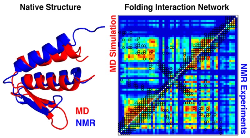
To investigate the unfolding of gpW in more depth, we turned to the analysis of residue–residue thermodynamic couplings. This method was originally devised for inferring the interaction network of one-state (global) downhill folding proteins from equilibrium NMR unfolding experiments.³¹ The degree of coupling between every pair of residues is thus obtained from the similarities among the unfolding patterns of all the possible CS-curve pairs (see the Methods section for details). A strong coupling between two residues is interpreted as indicative of concerted unfolding, whereas a weaker coupling implies uncorrelated unfolding events (e.g., residues with very different T_m).³¹ Primary couplings are between residues interacting in the native structure, and secondary couplings occur when the two residues are indirectly connected through mutual interactions with others. The approach is directly extensible to the NMR data of gpW because it is atomistically complex (Figure 1, Table S2), and is also transferable to the simulations, since we have computed CS thermal unfolding curves for all the relevant atoms. Figure 5 shows the thermodynamic coupling matrices resulting from the NMR experiments (left) and simulations (right). Both the experimental and simulation-based matrices exhibit a complex pattern of high (red), intermediate (yellow), and low (blue) couplings, indicating that at the residue level there still is significant variation in unfolding behaviors.

Figure 5.

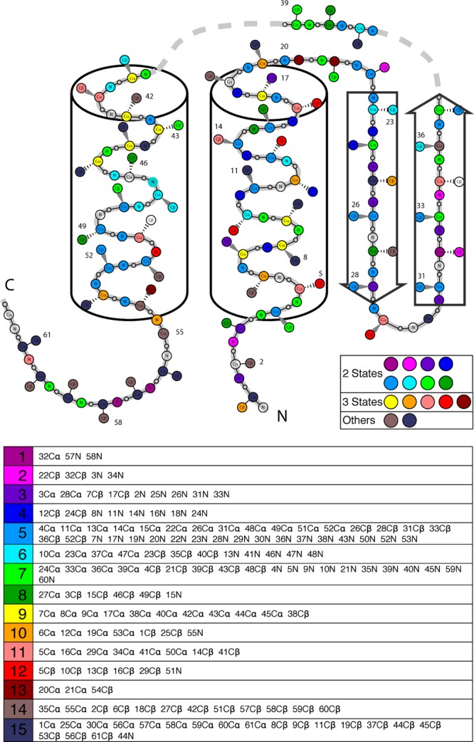
Mapping the folding interaction network of gpW from the residue–residue thermodynamic coupling matrix. Upper panels show the experimental (left column) and simulation-based (right column) residue–residue thermodynamic coupling matrix (highest coupling in red, lowest in dark blue), with native contacts identified using hollow black circles. The bottom right triangle shows the entire coupling matrix, while the upper left triangle shows only primary couplings (interacting residues). The structural and sequence distribution of the overall degree of coupling (defined as the sum of the couplings of a given residue to all other residues) is shown in the intermediate and bottom panels. Residues were classified in six levels of coupling (from low to high: dark blue, light blue, cyan, yellow, orange, red) using data clustering tools.

As first step in this analysis, we take advantage of the MD simulation results to better understand and test the mechanistic connection between the thermodynamic coupling matrix and the underlying folding interaction network. This is an important issue that could not be examined before because the NMR experimental data does not provide the structural information about the folding mechanism that is readily obtained from the simulated trajectories. Along these lines, we find that the thermodynamic information encoded in the simulated coupling matrix (Figure 5, right) agrees with the mechanistic information obtained from the kinetic clustering of the simulations (Figure 3B). Kinetic clustering shows that the β-hairpin is flexible in the native state, and unstructured in all other clusters (the only exception is M1, in which the hairpin is the only formed structure). Consistently, the hairpin is virtually uncoupled to everything else (Figure 5, right) and has the lowest melting temperature (Figure 4E). Thus, the structural element with lowest thermodynamic stability in the simulations forms last during folding and is also the least coupled to other protein regions in the matrix.

The two helices can be either formed or frayed in various clusters, but when they are formed, they tend to be formed for their full length (see I1, I2, and M2 in Figure 3), in agreement with their strong local coupling (Figure 5, right). Helix 1, which is better defined structurally than helix 2 in all clusters, exhibits stronger secondary couplings. The presence of interactions between the end of helix 1 and beginning of helix 2 in multiple clusters (Native, I2, and to a lesser extent, I1) is consistent with the strong interhelix coupling in the matrix, while the very transient interactions between the protein ends are consistent with their weak coupling observed in the matrix. Overall, the simulation results provide compelling support for the utility of residue–residue coupling matrices as an analytical tool for probing protein folding interaction networks. Moreover, the computed coupling matrix provides a picture of the folding process in simulation, in which individual helices can form independently of global folding, that is consistent with the simulated IR relaxation profiles (Figure 4B) and the kinetic clustering analysis (Figure 3B). This consistency further supports the use of equilibrium denaturation CS measurements as a way to obtain residue–residue coupling information and infer details of folding mechanisms.

As second step, we examine the similarities and differences between the experimental and simulated coupling matrices. This exercise is highly instructive from the viewpoint of evaluating and enhancing force field accuracy. Figure 5 shows that the simulated and experimental matrices do indeed share their main features. As in the simulation-based coupling matrix, for example, the experimental matrix identifies strong coupling between the end of helix 1 and the loop and the beginning of helix 2, as well as marginal coupling between the protein ends and between the β-hairpin and the rest of the protein. Moreover, high local coupling is found in the helical regions. At the residue level the similarities are notable to the extent that the simulations correctly capture the polarized distribution of strongly and weakly coupled residues along the length of the two helices and the hairpin (see the color patterns plotted on the gpW structure; Figure 5 middle). Such similarities indicate that the simulations reproduce the major structural and mechanistic aspects of gpW (un)folding.

Certain differences between the experimental and simulation-based coupling matrices emerge, however, when inspected in more depth. In the experiment, the residues with high overall coupling are more scattered throughout the sequence (Figure 5, bottom) whereas in the simulation, coupling tends to concentrate in the two helices (Figure , bottom), consistent with the observation of a less cooperative unfolding process (Figure 4D,E). In particular, the simulations do not capture a critical structural node that includes the hinge connecting the hairpin with helix 2 (L2, residues 35–41) and the middle of helix 1 (H1M, residues 7–15). This node appears to be key for the cooperative unfolding seen experimentally. For instance, L2 and H1M couple with the other hinge (residues 19–24) and the beginning of helix 2 (residues 41–48) through primary contacts. Strong secondary couplings (red-orange squares with no contacts) then link both segments to the remainder of both helices and to some residues in the first half of the hairpin, thus expanding the network over most of the protein.

In summary, while the simulations and the NMR experiments give consistent results with regard to the main aspects of the folding process, with early formation of helices and late formation of the hairpin, the simulated thermal unfolding process is more decoupled at the level of secondary structure elements than that demonstrated experimentally, providing a structural basis for the decreased cooperativity observed in simulations (Figures 3 and 4). We speculate that the higher stability of isolated secondary structure elements in simulation may result in a free energy surface containing more metastable states than observed experimentally. A possible reason for this discrepancy is that current force fields and water models tend to produce unfolded states that are too collapsed,^54,55 and this collapse may lead to overstabilization of individual secondary structure elements,^56,57 making the folding transition less cooperative.

Conclusions

Theory and simulations have suggested that complex folding mechanisms may still result in global two-state kinetics,^20,21,58,59 but obtaining experimental evidence for this type of conjecture has been challenging, since it requires the use of a method that provides a level of structural detail comparable to that of atomistic simulations. The NMR experiments reported here constitute a step in that direction, revealing that the apparently simple and cooperative global unfolding behavior of the protein gpW, which is in many ways consistent with two-state folding (and thus in principle an all-or-none process), hides a far richer process at the atomic level. The combination of experiments and simulations demonstrates that analysis of such atomistic details obtained from NMR data in terms of residue–residue coupling matrices, a technique that was originally developed for the investigation of one-state downhill folding mechanisms,³¹ provides important information related to the folding interaction network and mechanism of gpW. Moreover, the inherent features of gpW folding indicate that the experimental determination of residue–residue coupling matrices by NMR should be broadly applicable to fast folding proteins, even if they fold by crossing a free energy barrier. Practically, the reach of the method will be determined by the interplay between two interrelated parameters. First, the folding rate of the protein must be considerably faster than the chemical shift time scale (i.e., rates higher than ∼1/(200 μs)) to ensure fast-exchange NMR conditions. The second parameter is the intrinsic degree of folding cooperativity, because above a certain threshold the atomic heterogeneity might be indistinguishable from experimental uncertainty.⁶⁰ As the rate slows down, folding cooperativity will concomitantly increase, and thus the NMR analysis of sharper, more challenging unfolding transitions will also encounter decreased resolution due to line broadening. Nevertheless, there is nowadays an ample collection of single-domain proteins that have been experimentally identified to fold in microseconds and which contains examples from all major structural classes. This NMR experimental procedure thus emerges as a new approach to the characterization of folding interaction networks and as a complement to MD simulations in addressing the longstanding challenge of characterizing the folding and unfolding of proteins with atomic resolution.

Methods

Protein Production

A sequence containing residues 1–62 of the original gpW gene described by Davidson and co-workers⁶¹ was subcloned into the expression vector pBAT. Both unlabeled and uniformly ¹⁵N- and ¹³C-labeled gpW protein were produced using the same procedures previously described.³⁸

Circular Dichroism Spectroscopy

thermal unfolding experiments monitored by far-UV circular dichroism were performed on a Jasco J-815 spectropolarimeter equipped with Peltier thermal control using a 1 mm path-length cuvette. The samples were prepared at a protein concentration of 30 μM in 20 mM citrate buffer adjusted to pH 3.5.

NMR analysis and structure determination

NMR samples of ¹³C,¹⁵N-labeled gpW were prepared in a Shigemi tube at 1 mM concentration in 20 mM glycine buffer, 0.1 mM NaN₃, pH 3.5, 5% D₂O/H₂O and 100% D₂O. Under these conditions our gpW construct remained soluble and monomeric according to NMR line width values. NMR experiments were acquired at 294 K in a Bruker Avance III 600 MHz spectrometer equipped with a triple resonance z-axial-gradient probe. Sequence backbone chemical shift assignments were obtained from the following experiments: [¹H–¹⁵N] HSQC, HNCO, HNCACB, and CBCA(CO)NH. Side chain ¹H, ¹⁵N, and ¹³C assignments were obtained from HBHA(CO)NH, H(CCO)NH, C(CO)NH, and HCCH-TOCSY. NOE data were obtained from 3D ¹⁵N-HSQC-NOESY and 4D ¹³C-HMQC-NOESY using a mixing time of 110 ms. All experiments were processed with NMRPipe⁶² and analyzed with PIPP.⁶³ For the structure determination of gpW, experimental restraints derived from NOE cross-peaks, hydrogen bond distances, and dihedral angles were obtained. Only unambiguous interproton distance restraints were used, and errors of 25% of the distances were applied to obtain lower and upper distance limits. Hydrogen bond distance restraints (r_NH–O = 1.9–2.5 Å, r_N–O = 2.8–3.4 Å) were defined according to the experimentally determined secondary structure of the protein. The program TALOS+ was used to obtain 94 ϕ and ψ backbone torsion angle constraints for those residues with statistically significant predictions.⁶⁴ Structure calculations were performed with the program X-PLOR-NIH 2.16.0 by minimizing a target function that includes an harmonic potential for experimental distance restraints, a quadratic van der Waals repulsion term for the nonbonded contacts, and a square potential for torsion angles.⁶⁵ Starting structures were calculated and heated to 3000 K and cooled in 30 000 steps of 0.002 ps during simulated annealing. The final ensemble of 20 NMR structures was selected based on lowest energy and no restraint-violation criteria. These conformers had no distance restraint violations and no dihedral angle violations greater than 0.3 Å and 5°, respectively. Structures were validated using PROCHECK-NMR and MolProbity,^66,67 which show that the family of 20 structures are of considerable high quality in terms of geometry (92.6% of the residues populating the most favored regions of the Ramachandran plot for the whole ensemble) and side chain packing. Structures were analyzed with PyMOL(DeLano Scientific, San Carlos, CA). Coordinates were deposited in the Protein Data Bank with accession code 2L6R and chemical shifts were deposited in the Biological Magnetic Resonance Bank (BMRB code 17322).

NMR pH Titration

We obtained the chemical shift values of the side chain CO carbons of all Asp and Glu residues in gpW by analyzing a series of H(CA)CO spectra, a 2D version of the HCACO experiment.⁶⁸ The ¹Hε1 chemical shifts of the His15 were determined from a series of [¹H–¹³C] HSQC spectra.⁶⁹ All the spectra were recorded on an ∼1 mM ¹³C,¹⁵N-double labeled gpW sample, 0.1 mM DSS in D₂O at different pHs ranging from 1.5 to 8.1 (8.11, 7.16, 6.01, 5.09, 4.08, 3.57, 3.02, 1.98 and 1.53) and 294 K. NMR spectra were analyzed with SPARKY.^ref70 The pK_a values were obtained by a nonlinear least-squares fit of the experimental pH titration curves to the following equation:

where δ₁ and δ₂ are the chemical shift values at the lowest and highest pH, respectively. Data fitting was done with Origin Pro 8.0 (OriginLab).

Equilibrium Thermal Unfolding of gpW by NMR

As a first step, the reversibility of gpW thermal unfolding at the protein concentrations required for multidimensional NMR experiments was assessed using a NMR sample consisting of 1 mM ¹⁵N-labeled gpW in 20 mM glycine buffer, 0.1 mM NaN₃, pH 3.5, 5% D₂O/H₂O. This sample was heated up to 100 °C for a period of 2 h and then cooled back down. The perfect cross-peaks superimposition of the two [¹H–¹⁵N] HSQC spectra recorded before and after heating, indicated full reversibility in the relevant conditions. Equilibrium thermal unfolding was investigated using multidimensional NMR experiments to monitor the changes in ¹H, ¹⁵N, and ¹³C chemical shifts in the 273–371 K temperature range. For this purpose we used a Bruker 5 mm TXI-probe with z-axis gradient able to stand up to 423 K and a BTO temperature control unit. Accurate temperature calibration was carried out monitoring the ethylene glycol CS at every experimental temperature using a sample of ethylene glycol prepared in a regular 5 mm diameter NMR tube and using an air flow-rate of 535 L/h and following the procedure described by Amman et al.⁷⁰ Briefly, the neat ethylene glycol sample was equilibrated for 30 min at each temperature before acquiring the spectrum. Standard one-pulse 1D ¹H NMR experiments were used to monitor the changes in proton frequency of −CH₂– and −OH with temperature. These changes were converted to temperature using equation: T(K) = 466.5 – 102.00 Δδ. For the thermal unfolding experiments we employed a NMR sample at 1 mM concentration of ¹³C,¹⁵N-labeled gpW in 20 mM glycine buffer, 0.1 mM NaN₃, 0.01 DSS, pH 3.5, 5% D₂O/H₂O. In these experiments the water resonance was used as spectral reference since the observation of the standard DSS signal is precluded in multidimensional NMR experiments because of isotope filtering. Thus, before recording the set of multidimensional experiments, a 1D ¹H NMR experiment was recorded and employed to calibrate the position of the water signal relative to DSS at each temperature. Pressurizable tubes manufactured by New Era Enterprises (U.S.) with 0.77 mm thick glass were used to minimize evaporation of the sample. We measured the pH of NMR samples at the different experimental temperatures using a thermal block and a pH-meter recalibrated at each temperature. We observed that the pH of the samples was held constant at a value of 3.5 ± 0.1 over the whole temperature range. Protein backbone amide ¹⁵N, ¹H^N, ¹³Cα, and ¹³Cβ chemical shifts were assigned with the following set of experiments: [¹H–¹⁵N] HSQC, CBCA(CO)NH, and HNCACB. GpW folds in fast exchange regime relative to the NMR chemical shift time scale, and thus, each atom produces a single chemical shift corresponding to the dynamically averaged conformational ensemble at every condition. The ensemble average chemical shifts for all relevant atoms were fully assigned in the 273–371 K temperature range at fixed intervals of 5 K. At temperature conditions within the unfolding transition region (slightly below and above the T_m) the temperature interval for NMR experiments was reduced to 3 K to increase the data density in the region of largest change in CS. All experiments were processed with NMRPipe and analyzed with PIPP to obtain accurate chemical shift determinations using a multilevel contour averaging procedure. At pH 3.5 and high temperatures gpW experienced slow proteolysis at specific positions in the primary sequence involving glutamine residues. We thus monitored protein integrity by comparing [¹H–¹⁵N] HSQC spectra recorded before and after every set of triple-resonance NMR experiments. At temperatures higher than 345 K the gpW proteolysis rate was higher than 1/(5 days) so we used a freshly prepared sample for recording the suite of triple resonance NMR experiments at each temperature above 345 K.

Fast-Folding Kinetics by Nanosecond Laser-Induced T-Jump

folding-unfolding relaxation kinetics of gpW was measured using a nanosecond laser-induced T-jump apparatus equipped with infrared detection. Samples were prepared at 4 mg/mL concentration in 20 mM deuterated glycine buffer, after multiple cycles of liophilization and dilution in D2O to achieve complete deuteration of the exchangeable amide protons. The buffer and sample were adjusted to pD = 3.5, correcting for the isotope effect on the glass electrode readout. The relaxation kinetics of gpW after a jump of ∼10 K to a final temperature of 328 K were recorded on a custom-built infrared laser-induced temperature apparatus described previously.¹⁸ Briefly, the fundamental wavelength of a Nd:YAG laser (Continuum Surelite I) operating at a repetition rate of 4 Hz is shifted, by passing through a 1m path Raman cell (Lightage inc.) filled with a high pressure mixture of H₂ and Ar, to 1907 nm, resonant with the infrared absorption of D₂O. In this way pulses <10 ns with energy of up to 30 mJ were obtained, that induced a local temperature jump of about 10–12° when focused onto the sample. The folding-unfolding relaxation kinetics of gpW was observed using a quantum cascade laser (Daylight Solutions) tuned to 1632 cm^–1 to match the absorption of the α helix signal within the gpW amide I band. The light transmitted from the sample was recorded using a fast MCT detector (Kolmar Technologies) coupled with an oscilloscope (Tektronix DPO4032). Samples were held in a cell formed by two MgF₂ windows separated by a 50 μm Teflon spacer and thermostated at the proper base temperature using two Peltier thermoelectric coolers (TE Technology Inc.) in a custom-built sample holder. The transmission of D₂O was used as an internal thermometer to measure the amplitude of the temperature jump.

MD Simulations

Molecular dynamics (MD) simulations of gpW were initiated in an extended conformation. The 62-amino acids sequence MVRQEELAAARAALHDLMTGKRVATVQKDGRRVEFTATSVSDLKKYIAELEVQTGMTQRRRG was solvated in a cubic 60 × 60 × 60 ų box, containing 6345 water molecules and 15 mM NaCl. Asp, Glu, Arg, Lys, and His residues were treated as charged. The CHARMM-h force field^71,72 (see SOM) was used to represent the system. The system was initially equilibrated at 340 K and 1 bar in the NPT ensemble. Production runs were performed with the Anton specialized hardware⁴³ using a 2.5 fs time step. Bonds involving hydrogen atoms were restrained to their equilibrium lengths using the M-SHAKE algorithm.⁷³ Nonbonded interactions were truncated at 10 Å, and an Ewald method was used to describe the long-range electrostatic interactions.⁷⁴ Four simulated tempering⁷⁵ simulations of 200 μs each, were performed in the NPT ensemble.⁷⁶⁻⁷⁸ Two simulations used 18 temperature intervals between 278 and 398 K, and two used 21 temperature intervals between 278 and 438 K. Exchanges between temperatures were attempted every 20 ps of simulation. To gain additional kinetic information, we also performed a 258 μs equilibrium MD simulation at 340 K in the NVT ensemble. A kinetic clustering analysis was used to identify the most relevant metastable states on the free-energy surface through a fit of the autocorrelation functions of 400 Cα–Cα contacts on time scales ranging from 0.5 to 50 μs.^16,45 In order to obtain consistent clustering, this analysis was simultaneously performed on the five trajectories combined. Chemical shift predictions were performed using the CamShift⁵² and SPARTA+⁵³ programs. Helical residues for the analysis of the autocorrelation function were identified according to the STRIDE definition,⁷⁹ as implemented in VMD.

Analysis of Experimental CS Curves

as a first step, all obtained experimental CS curves were classified in three groups according to the unfolding behavior: (1) 102 curves were classified as 2-state-like (2SL) curves because they had a distinctly sigmoidal trend characterized by a single transition and a single peak in their derivative; (2) 35 curves were classified as 3-state-like (3SL) because they exhibited two apparent transitions and thus a bisigmoidal shape and two peaks in their derivative; and (3) 43 curves did not fit any of the other two categories (whether because they exhibited multiple transitions or no obvious transition), and were thus included in the complex-pattern (CP) group. The CS curves classified as 2SL and 3SL were fitted to a thermodynamic two-state or a three-state unfolding model equation, respectively, using the procedures described previously.⁴⁰

Cluster Analysis of CS Curves

The data set containing all of the experimental CS curves was analyzed globally using data clustering methods. CS curves belonging to the 2SL and 3SL groups were clustered according to both the thermodynamic parameters obtained in their fits (T_m and ΔH for 2SL and T_m1, T_m2, ΔH₁, and ΔH₂ for 3SL) or according to the probability of the native state as a function of temperature obtained from the two and three fits. Both methods rendered equivalent results. CS curves included in the CP group were clusterized according to their similarity after normalization of the signal using the Z-score procedure.⁴⁰ All clustering routines were performed with the kmeans algorithm by running 10 000 trials to guarantee convergence and selecting the solution with minimum residuals. The 102 2SL curves were clustered into 12 clusters, out of which 8 clusters had at least 3 elements, whereas the other 4 clusters had only 1 or 2 elements. Clustering of the 35 3SL curves produced 5 clusters with at least 3 elements. CP curves were grouped in 10 clusters by kmeans according to their zscored shape, out of which only 2 clusters had 3 elements or more. Using these procedures, a total of 15 characteristic clusters were identified with at least three elements containing in total 132 atomic unfolding curves. The main cluster properties are summarized in Tables S6–S8.

Residue–Residue Thermodynamic Coupling Matrices from Experiment and Simulations

The thermodynamic coupling index (TCI) for each pair of residues in a protein is calculated from the pairwise comparison between all the CS curves of the first residue in the pair with all the curves of the second residue. The thermodynamic coupling index of residues x and y is then calculated by summing all the possible pairwise comparisons of atomic folding curves as reported in the following equation:

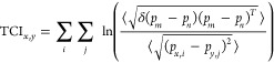where p_m and p_n are row vectors from a matrix including all the zscored CS curves in the protein. The numerator thus corresponds to the mean RMSD for all CS curves in the data set. P_x,i and p_y,j are the vectors from the same matrix that correspond to the CS curves of residues x and y, respectively (i runs over all curves of residue x and j over all curves of residue y). The TCI for residues x and y is positive when the average Euclidean distance between all their cross-pairs is smaller than the mean RMSD for all CS curves in the protein and negative otherwise. The TCI matrix is constructed by repeating the same procedure over all possible residue pairs. This procedure was applied to both the experimental CS curves measured by NMR and the synthetic CS curves computed with either CamShift⁵² or SPARTA+⁵³ from all the conformations observed at each temperature in the ST simulations.

Supporting Information Available

Figures S1–S5 and Tables S1–S9. The Supporting Information is available free of charge on the ACS Publications website at DOI: 10.1021/jacs.5b02324.

Author Present Address

^⊥ L.S.: Biozentrum, University of Basel, Switzerland

Author Present Address

^# A.V.: Steinbuch Centre for Computing, Karlsruhe Institute of Technology, Karlsruhe, Germany

Author Present Address

^⊗ K.L.-L.: Structural Biology and NMR Laboratory (SBiNLab), Department of Biology, University of Copenhagen, DK-2200 Copenhagen, Denmark

The authors declare no competing financial interest.

References

- Wolynes P. G.; Onuchic J. N.; Thirumalai D. Science 1995, 267, 1619. [DOI] [PubMed] [Google Scholar]
- Best R. B.; Hummer G.; Eaton W. A. Proc. Natl. Acad. Sci. U.S.A. 2013, 110, 17874. [DOI] [PMC free article] [PubMed] [Google Scholar]
- Koga N.; Tatsumi R.; Liu G.; Xiao R.; Acton T. B.; Montelione G. T.; Baker D. Nature 2012, 491, 222. [DOI] [PMC free article] [PubMed] [Google Scholar]
- Jackson S. E. Folding Des. 1998, 3, R81. [DOI] [PubMed] [Google Scholar]
- Rhoades E.; Cohen M.; Schuler B.; Haran G. J. Am. Chem. Soc. 2004, 126, 14686. [DOI] [PubMed] [Google Scholar]
- Stigler J.; Ziegler F.; Gieseke A.; Gebhardt J. C. M.; Rief M. Science 2011, 334, 512. [DOI] [PubMed] [Google Scholar]
- Elms P. J.; Chodera J. D.; Bustamante C.; Marqusee S. Proc. Natl. Acad. Sci. U.S.A. 2012, 109, 3796. [DOI] [PMC free article] [PubMed] [Google Scholar]
- Chung H. S.; McHale K.; Louis J. M.; Eaton W. A. Science 2012, 335, 981. [DOI] [PMC free article] [PubMed] [Google Scholar]
- Chung H. S.; Eaton W. A. Nature 2013, 502, 685. [DOI] [PMC free article] [PubMed] [Google Scholar]
- Yang W. Y.; Gruebele M. Nature 2003, 423, 193. [DOI] [PubMed] [Google Scholar]
- Prigozhin M. B.; Gruebele M. Phys. Chem. Chem. Phys. 2013, 15, 3372. [DOI] [PMC free article] [PubMed] [Google Scholar]
- Hu W.; Walters B. T.; Kan Z.-Y.; Mayne L.; Rosen L. E.; Marqusee S.; Englander S. W. Proc. Natl. Acad. Sci. U.S.A. 2013, 110, 7684. [DOI] [PMC free article] [PubMed] [Google Scholar]
- Eaton W. A.; Muñoz V.; Hagen S. J.; Jas G. S.; Lapidus L. J.; Henry E. R.; Hofrichter J. Annu. Rev. Biophys. Biomol. Struct. 2000, 29, 327. [DOI] [PMC free article] [PubMed] [Google Scholar]
- Serrano A. L.; Waegele M. M.; Gai F. Protein Sci. 2012, 21, 157. [DOI] [PMC free article] [PubMed] [Google Scholar]
- Schuler B.; Hofmann H. Curr. Opin. Struct. Biol. 2013, 23, 36. [DOI] [PubMed] [Google Scholar]
- Shaw D. E.; Maragakis P.; Lindorff-Larsen K.; Piana S.; Dror R. O.; Eastwood M. P.; Bank J. A.; Jumper J. M.; Salmon J. K.; Shan Y.; Wriggers W. Science 2010, 330, 341. [DOI] [PubMed] [Google Scholar]
- Piana S.; Lindorff-Larsen K.; Shaw D. E. Science 2011, 334, 517. [DOI] [PubMed] [Google Scholar]
- Fung A.; Li P.; Godoy-Ruiz R.; Sanchez-Ruiz J. M.; Muñoz V. J. Am. Chem. Soc. 2008, 130, 7489. [DOI] [PubMed] [Google Scholar]
- Naganathan A. N.; Muñoz V. Biochemistry 2008, 47, 6752. [DOI] [PubMed] [Google Scholar]
- Voelz V. A.; Bowman G. R.; Beauchamp K.; Pande V. S. J. Am. Chem. Soc. 2010, 132, 1526. [DOI] [PMC free article] [PubMed] [Google Scholar]
- Beauchamp K. A.; R M.; Y.-S L.; Pande V. S. Proc. Natl. Acad. Sci. U.S.A. 2012, 109, 17807. [DOI] [PMC free article] [PubMed] [Google Scholar]
- Korzhnev D. M.; Religa T. L.; Banachewicz W.; Fersht A. R.; Kay L. E. Science 2010, 329, 1312. [DOI] [PubMed] [Google Scholar]
- Bouvignies G.; Vallurupalli P.; Hansen D. F.; Correia B. E.; Lange O.; Bah A.; Vernon R. M.; Dahlquist F. W.; Baker D.; Kay L. E. Nature 2011, 477, 111. [DOI] [PMC free article] [PubMed] [Google Scholar]
- Hansen D. F.; Vallurupalli P.; Lundstrom P.; Neudecker P.; Kay L. E. J. Am. Chem. Soc. 2008, 130, 2667. [DOI] [PubMed] [Google Scholar]
- Sanchez-Medina C.; Sekhar A.; Vallurupalli P.; Cerminara M.; Muñoz V.; Kay L. E. J. Am. Chem. Soc. 2014, 136, 7444. [DOI] [PubMed] [Google Scholar]
- Muñoz V. Annu. Rev. Biophys. Biomol. Struct. 2007, 36, 395. [DOI] [PubMed] [Google Scholar]
- Li P.; Oliva F. Y.; Naganathan A. N.; Muñoz V. Proc. Natl. Acad. Sci. U.S.A. 2009, 106, 103. [DOI] [PMC free article] [PubMed] [Google Scholar]
- Muñoz V. Int. J. Quantum Chem. 2002, 90, 1522. [Google Scholar]
- Naganathan A. N.; Perez-Jimenez R.; Sanchez-Ruiz J. M.; Muñoz V. Biochemistry 2005, 44, 7435. [DOI] [PubMed] [Google Scholar]
- Garcia-Mira M. M.; Sadqi M.; Fischer N.; Sanchez-Ruiz J. M.; Muñoz V. Science 2002, 298, 2191. [DOI] [PubMed] [Google Scholar]
- Sadqi M.; Fushman D.; Muñoz V. Nature 2006, 442, 317. [DOI] [PubMed] [Google Scholar]
- Ferguson N.; Sharpe T. D.; Schartau P. J.; Sato S.; Allen M. D.; Johnson C. M.; Rutherford T. J.; Fersht A. R. J. Mol. Biol. 2005, 353, 427. [DOI] [PubMed] [Google Scholar]
- Mayor U.; Grossmann J. G.; Foster N. W.; Freund S. M.; Fersht A. R. J. Mol. Biol. 2003, 333, 977. [DOI] [PubMed] [Google Scholar]
- Ferguson N.; Sharpe T. D.; Johnson C. M.; Schartau P. J.; Fersht A. R. Nature 2007, 445, E14. [DOI] [PubMed] [Google Scholar]
- Zhou Z.; Bai Y. Nature 2007, 445, E16. [DOI] [PubMed] [Google Scholar]
- Onuchic J. N.; Wolynes P. G. Curr. Opin. Struct. Biol. 2004, 14, 70. [DOI] [PubMed] [Google Scholar]
- Klimov D. K.; Thirumalai D. J. Comput. Chem. 2002, 23, 161. [DOI] [PubMed] [Google Scholar]
- Sborgi L.; Verma A.; Muñoz V.; de Alba E. PLoS One 2011, 6, e26409. [DOI] [PMC free article] [PubMed] [Google Scholar]
- Wishart D. S.; Nip A. M. Biochem. Cell Biol. 1998, 76, 156. [DOI] [PubMed] [Google Scholar]
- Sborgi L.; Verma A.; Sadqi M.; de Alba E.; Muñoz V. Methods Mol. Biol. 2013, 932, 205. [DOI] [PubMed] [Google Scholar]
- Best R. B. Curr. Opin. Struct. Biol. 2012, 22, 52. [DOI] [PubMed] [Google Scholar]
- Gruebele M. In Protein Folding, Misfolding and Aggregation. Classical Themes and Novel Approaches; Muñoz V., Ed.; RSC: Cambridge, 2008. [Google Scholar]
- Shaw D. E.; Dror R. O.; Salmon J. K.; Grossman J. P.; Mackenzie K. M.; Bank J. A.; Young C.; Deneroff M. M.; Batson B.; Bowers K. J.; Chow E.; Eastwood M. P.; Ierardi D. J.; Klepeis J. L.; Kuskin J. S.; Larson R. H.; Lindorff-Larsen K.; Maragakis P.; Moraes M. A.; Piana S.; Shan Y.; Towles B.. Conference on High Performance Computing, Networking, Storage and Analysis (SC09); ACM: New York, NY, 2009. [Google Scholar]
- Piana S.; Lindorff-Larsen K.; Shaw D. E. Proc. Natl. Acad. Sci. U.S.A. 2012, 109, 17845. [DOI] [PMC free article] [PubMed] [Google Scholar]
- Piana S.; Lindorff-Larsen K.; Shaw D. E. Proc. Natl. Acad. Sci. U.S.A. 2013, 110, 5915. [DOI] [PMC free article] [PubMed] [Google Scholar]
- Piana S.; Lindorff-Larsen K.; Shaw D. E. J. Phys. Chem. B 2013, 117, 12935. [DOI] [PubMed] [Google Scholar]
- Lindorff-Larsen K.; Maragakis P.; Piana S.; Eastwood M. P.; Dror R. O.; Shaw D. E. PLoS One 2013, 7, e32131. [DOI] [PMC free article] [PubMed] [Google Scholar]
- Frank A. T.; Law S. M.; Ahlstrom L. S.; Brooks C. L. J. Chem. Theory Comput. 2014, 11, 325. [DOI] [PMC free article] [PubMed] [Google Scholar]
- Nauli S.; Kuhlman B.; Baker D. Nat. Struct. Biol. 2001, 8, 602. [DOI] [PubMed] [Google Scholar]
- Snow C. D.; Nguyen H.; Pande V. S.; Gruebele M. Nature 2002, 420, 102. [DOI] [PubMed] [Google Scholar]
- Mark P.; Nilsson L. J. Phys. Chem. A 2001, 105, 9954. [Google Scholar]
- Kohlhoff K. J.; Robustelli P.; Cavalli A.; Salvatella X.; Vendruscolo M. J. Am. Chem. Soc. 2009, 131, 13894. [DOI] [PubMed] [Google Scholar]
- Shen Y.; Bax A. J. Biomol. NMR 2010, 48, 13. [DOI] [PMC free article] [PubMed] [Google Scholar]
- Piana S.; Klepeis J. L.; Shaw D. E. Curr. Opin. Struct. Biol. 2014, 24, 98. [DOI] [PubMed] [Google Scholar]
- Best R. B.; Zheng W.; Mittal J. J. Theory Comput. 2014, 10, 5113. [DOI] [PMC free article] [PubMed] [Google Scholar]
- Chen T.; Chan H. S. Phys. Chem. Chem. Phys. 2014, 16, 6460. [DOI] [PubMed] [Google Scholar]
- Piana S.; Lindorff-Larsen K.; Dirks R. M.; Salmon J. K.; Dror R. O.; Shaw D. E. PLoS One 2012, 7, e39918. [DOI] [PMC free article] [PubMed] [Google Scholar]
- Krivov S. V.; Karplus M. Proc. Natl. Acad. Sci. U.S.A. 2004, 101, 14766. [DOI] [PMC free article] [PubMed] [Google Scholar]
- Krivov S. V.; Muff S.; Caflisch A.; Karplus M. J. Phys. Chem. B 2008, 112, 8701. [DOI] [PMC free article] [PubMed] [Google Scholar]
- Maxwell K. L.; Davidson A. R.; Murialdo H.; Gold M. J. Biol. Chem. 2000, 275, 18879. [DOI] [PubMed] [Google Scholar]
- Delaglio F.; Grzesiek S.; Vuister G. W.; Zhu G.; Pfeifer J.; Bax A. J. Biomol. NMR 1995, 6, 277. [DOI] [PubMed] [Google Scholar]
- Garrett D. S.; A.M G.; G.M C. J. Magn. Reson. 1991, 95, 214. [Google Scholar]
- Shen Y.; Delaglio F.; Cornilescu G.; Bax A. J. Biomol. NMR 2009, 44, 213. [DOI] [PMC free article] [PubMed] [Google Scholar]
- Schwieters C. D.; Kuszewski J. J.; Tjandra N.; Clore G. M. J. Magn. Reson. 2003, 160, 65. [DOI] [PubMed] [Google Scholar]
- Davis I. W.; Leaver-Fay A.; Chen V. B.; Block J. N.; Kapral G. J.; Wang X.; Murray L. W.; Arendall W. B. III; Snoeyink J.; Richardson J. S.; Richardson D. C. Nucleic Acids Res. 2007, 35, W375. [DOI] [PMC free article] [PubMed] [Google Scholar]
- Laskowski R. A.; Rullmannn J. A.; MacArthur M. W.; Kaptein R.; Thornton J. M. J. Biomol. NMR 1996, 8, 477. [DOI] [PubMed] [Google Scholar]
- Kay L. E.; Ikura M.; Tschudin R.; Bax A. J. Magn. Reson. 1990, 89, 496. [DOI] [PubMed] [Google Scholar]
- Bax A.; Ikura M.; Kay L. E.; Torchia D. A.; Tschudin R. J. Magn. Reson. 1990, 86, 304. [DOI] [PubMed] [Google Scholar]
- Goddard T. D.; Kneller D. G.. SPARKY 3; University of California, San Francisco, 2008.
- Amman C.; Meier P.; Merbach A. E. J. Magn. Reson. 1982, 46, 319. [Google Scholar]
- MacKerell A. D. Jr.; Bashford D.; Bellott M.; Dunbrack R. L. Jr.; Evanseck J. D.; Field M. J.; Fischer S.; Gao J.; Guo H.; Ha S.; Joseph-McCarthy D.; Kuchnir L.; Kuczera K.; Lau F. T. K.; Mattos C.; Michnick S.; Ngo T.; Nguyen D. T.; Prodhom B.; Reiher W. E. III; Roux B.; Schlenkrich M.; Smith J. C.; Stote R.; Straub J.; Watanabe M.; Wiórkiewicz-Kuczera J.; Yin D.; Karplus M. J. Phys. Chem. B 1998, 102, 3586. [DOI] [PubMed] [Google Scholar]
- MacKerell A. D. Jr.; Feig M.; Brooks C. L. J. Comput. Chem. 2004, 25, 1400. [DOI] [PubMed] [Google Scholar]
- Krautler V.; van Gunsteren W. F.; Hunenberger P. H. J. Comput. Chem. 2001, 22, 501. [Google Scholar]
- Shan Y.; Klepeis J. L.; Eastwood M. P.; Dror R. O.; Shaw D. E. J. Chem. Phys. 2005, 122, 54101. [DOI] [PubMed] [Google Scholar]
- Marinari E.; Parisi G. Europhys. Lett. 1992, 19, 451. [Google Scholar]
- Nosé S. J. Chem. Phys. 1984, 81, 511. [Google Scholar]
- Hoover W. G. Phys. Rev. A 1985, 31, 1695. [DOI] [PubMed] [Google Scholar]
- Martyna G. J.; Tobias D. J.; LKlein M. L. J. Chem. Phys. 1994, 101, 4177. [Google Scholar]
- Frishman D.; Argos P. Proteins. Struct., Funct., Gen. 1995, 23, 566. [DOI] [PubMed] [Google Scholar]
Associated Data
This section collects any data citations, data availability statements, or supplementary materials included in this article.