Impermanence of dendritic spines in live adult CA1 hippocampus

Abstract

Mammalian hippocampus is crucial for episodic memory formation¹ and transiently retains information for ~3–4 weeks in adult mice and longer in humans². Although neuroscientists widely believe neural synapses are elemental sites of information storage³, there has been no direct evidence hippocampal synapses persist for time intervals commensurate with the duration of hippocampal-dependent memory. Here we tested the prediction that the lifetimes of hippocampal synapses match the longevity of hippocampal memory. By using time-lapse two-photon microendoscopy⁴ in the CA1 hippocampal area of live mice, we monitored the turnover dynamics of pyramidal neurons’ basal dendritic spines, post-synaptic structures whose turnover dynamics are thought to reflect those of excitatory synaptic connections^5,6. Strikingly, CA1 spine turnover dynamics differed sharply from that seen previously in neocortex^7–9. Mathematical modeling revealed that the data best matched kinetic models with a single population of spines of mean lifetime ~1–2 weeks. This implies ~100% turnover in ~2–3 times this interval, a near full erasure of the synaptic connectivity pattern. Although NMDA receptor blockade stabilizes spines in neocortex^10,11, in CA1 it transiently increased the rate of spine loss and thus lowered spine density. These results reveal that adult neocortical and hippocampal pyramidal neurons have divergent patterns of spine regulation and quantitatively support the idea that the transience of hippocampal-dependent memory directly reflects the turnover dynamics of hippocampal synapses.

The hypothesis that synaptic connectivity patterns encode information has profoundly shaped research on long-term memory. In hippocampus, synapses in basal CA1 mainly receive inputs from hippocampal area CA3, and the CA3 → CA1 projection has been widely studied regarding its plasticity and key role in memory. As in neocortex, dendritic spines in hippocampus are good proxies for excitatory synapses¹², motivating time-lapse imaging of spines as a means of monitoring synaptic turnover^7–10.

Prior work has illustrated in vivo imaging of CA1 spines in acute and recently also in chronic preparations^13–15. We tracked spines for up to ~14 weeks by combining microendoscopes of diffraction-limited resolution¹⁴ (0.85 NA), a chronic mouse preparation for time-lapse imaging in deep brain areas⁴, and Thy1-GFP mice that express green fluorescent protein (GFP) in a sparse subset of CA1 pyramidal neurons (Fig. 1, Extended Fig. 1). Histological analyses confirmed this approach induced minimal activation of glia (Extended Fig. 2), as shown previously^4,16.

Fig. 1. Dendritic spines are dynamic in CA1 hippocampus of the adult mouse.

(a) A sealed, glass guide tube implanted dorsal to CA1 allows time-lapse in vivo imaging of dendritic spines.

(b) A doublet microendoscope projects the laser scanning pattern onto the specimen plane in tissue. Inset: Red lines indicate optical ray trajectories.

(c) CA1 dendritic spines in a live Thy1-GFP mouse.

(d) Time-lapse image sequences. Arrowheads indicate spines that either persist across the sequence (white arrowheads), disappear midway (red), arise midway and then persist (green), arise midway and then later disappear (yellow), or disappear and then later appear at an indistinguishable location (cyan).

A major concern was that one cannot distinguish two or more spines spaced within two-photon microscopy’s resolution limit. This issue is critical for studies of hippocampal spines, which are more densely packed than neocortical spines¹⁷. To gauge how commonly spines’ appearances merged together, we examined tissue slices from Thy1-GFP mice, using both two-photon microendoscopy and stimulated-emission depletion (STED) microscopy. The latter offered super-resolution (~70 nm FWHM lateral resolution), nearly nine times finer than that of the former¹⁴ (~610 nm), permitting tests comparing pairs of images of the same CA1 dendrites (Fig. 2a, Extended Fig. 3).

Fig. 2. A simple kinetic model sufficed to describe CA1 pyramidal cell spine dynamics.

(a) Two-photon microendoscopy and stimulated emission depletion (STED) imaging of the same dendrites in vitro. (Top row) two-photon images depict spines closer than the resolution limit as merged entities. (Bottom) Asterisks mark example, visually scored spines, showing cases in which nearby spines do (right) or do not (left) merge.

(b) Fraction of spines (N = 151 total) seen by two-photon imaging, that were one, two or three spines as determined by STED imaging. Error bars: s.d.

(c) Separations between adjacent unmerged spines and pairs of spines that appeared merged by two-photon imaging. Open grey circles mark individual results from each of N = 150 spines. Black bars: mean ± s.d.

(d) Example, computer-simulated, time-lapse image sequence, used to quantify how resolution limits impact measured spine densities and dynamics.

(e) Computational modeling predicts the underestimation of spine density due to the finite optical resolution. Blue diagonal line: perfect detection of all spines. Black horizontal dashed lines: typical ranges of spine densities on pyramidal cells in neocortex and hippocampus. Red data: results from visually scoring simulated images of dendrites of varying spine densities. Black curve: prediction from the scoring model using 600 nm as the minimum separation between two spines correctly distinguished.

(f) Modeling predicts the overestimation of spine stability due to merging of adjacent spines in resolution-limited images. Blue data: Survival fraction values (mean ± s.e.m.) for actual spine turnover in computer simulations (spine density:2.56 μm⁻¹). Red data: Apparent turnover for these same simulated dendrites, as scored from simulated two-photon images. Black curves: Theoretical predictions for spine survival based on the scoring model.

As expected, we saw nearby spines in STED images that appeared merged in the two-photon images (Fig. 2a). 23 ± 3.6% (s.e.m.) of spines that appeared unitary in the two-photon images were actually two spines (Fig. 2b). 6.0 ± 1.6% were actually three spines. Distances between merged spines in the two-photon images (0.51 ± 0.14 μm; mean ± s.d.) were below the (0.61 μm) resolution limit¹⁴ (Fig. 2c). Plainly, merging can induce illusory spine stability, since two or more real spines must vanish for a merged spine to disappear.

To treat merging effects quantitatively, we developed a mathematical framework permitting systematic examination of turnover dynamics across different kinetic models and how merging of spines’ appearances alters the manifestations of these dynamics in two-photon imaging data (Supplementary Text; Extended Figs. 4–7). We used computer simulations to study how the density and apparent kinetics of merged spines vary with geometric variations of individual spines, spine density, resolution, and spine kinetics (Supplementary Text; Extended Fig. 8). We also checked experimentally if fluctuations in spine angle and length, and the radius of the dendrite near the spine might impact measures of spine turnover (Extended Figs. 6,9). By simulating time-lapse image series, we scored and analyzed synthetic data across a broad range of optical conditions, spine densities, geometries, and turnover kinetics (Fig. 2d; Extended Figs. 4,5).

The simulations and mathematical modeling confirmed that naïve analyses of two-photon data are inappropriate at the spine densities in CA1, due to merging and the resulting illusion of increased stability (Supplementary Text; Extended Fig. 4). For stability analyses, we followed prior studies^7–9 in our use of the survival fraction curve, S(t), the fraction of spines appearing in both the initial image acquired at t=0 and that at time t. The shape and asymptotic value of S(t) provide powerful constraints on kinetic models of turnover and the fraction of spines that are permanent (i.e. a rate constant of zero for spine loss)^7–9 (Supplementary Text). Strikingly, visual scoring of simulated images (Fig. 2d; Extended Fig. 5) yielded underestimates of spine density (Fig. 2e) and patent overestimates of spines’ lifetimes (Fig. 2f). But crucially, our treatment accurately predicted the relationship between the actual density and the visually determined underestimate, and properly explained the apparent turnover dynamics, S(t), in terms of the actual kinetics (Fig. 2f, Extended Figs. 5c and 7). Overall, the simulations showed face-value interpretations of two-photon images from CA1 are untrustworthy, but one can make quantitatively correct inferences about spine kinetics provided one properly accounts for the optical resolution. Using the same framework, we next analyzed real data.

Initial analyses focused on four mice in which we acquired image stacks of CA1 pyramidal cells and tracked spines every three days for 21 days [60 dendrites total; 50 ± 7 (mean ± s.d.) per session] (Fig. 3a). Whenever individual spines appeared at indistinguishable locations on two or more successive sessions, we identified these as observations of the same spine. Overall, we made 4903 spine observations [613 ± 71 (mean ± s.d.) per day]. Spine densities were invariant over time (Fig. 3b) (Wilcoxon signed-rank test; n = 16–50 dendrites per comparison of a pair of days; significance threshold = 0.0018 after Dunn-Šidák correction for 28 comparisons; P > 0.047 for all comparisons), as were spine volumes (P = 0.87; Kruskal-Wallis ANOVA) (Extended Fig. 10), and the turnover ratio, the fraction of spines arising or vanishing since the last session⁷ (Fig. 3b) (Wilcoxon signed-rank test; 14–40 dendrites; significance threshold = 0.0025 after correction for 20 comparisons; P > 0.31 for all comparisons). Under 50% of spines (46 ± 2%; mean ± s.e.m.; n = 4 mice) were seen throughout the experiment (Extended Fig. 1d,e), although our simulations had shown this naïve observation overestimated spine stability.

Fig. 3. NMDA receptor blockade, but not environmental enrichment, altered spine turnover dynamics.

(a) Schedule of baseline imaging sessions.

(b) Neither measured spine densities (upper) nor turnover ratios (lower) varied for mice in their home cages. Horizontal lines: Mean spine density and turnover ratio

(c) Spine survival (upper) and newborn spine survival (lower).

(d) Schedule for study on environmental enrichment.

(e, f) No significant differences existed between baseline (black points) and enriched conditions (red) regarding spine density, (e, upper), turnover, (e, lower), survival, (f, upper), or newborn spine survival, (f, lower).

(g) Schedule for the study on NMDA receptor blockade..

(h) MK801 caused a significant decline in spine density. Data are from mice imaged four times before (black) and six times during (green) MK801 administration. Black and green horizontal lines respectively indicate mean densities during baseline the last four days of MK801 treatment. The density decrease was highly significant (Wilcoxon signed-rank test; n = 29 dendrites; P = 0.0007).

(i) The decline in spine density early in MK801 treatment arose from a transient, highly significant difference between the rates at which spines were lost (darker bars) and gained (lighter bars) (Wilcoxon signed-rank test; n = 29 dendrites; P = 0.0008). Grayscale and green shaded bars represent percentages of spines gained and lost for sessions prior to and during MK801 dosage.

All error bars are s.e.m.

The time-invariance of spine densities and turnover ratios implied that via our mathematical framework we could determine the underlying kinetic parameters governing turnover. S(t) curves for the total and newborn spine populations ostensibly resembled those reported for neocortex^7–9 (Fig. 3c). However, unlike in neocortex, the 46% of spines seen in all sessions differed notably from the odds that a spine was observed twice in the same location across two distant time points, as quantified by the asymptotic value of S(t) (73 ± 3%). This discrepancy suggested that, as our modeling had indicated, many CA1 spines might vanish and re-appear in an ongoing way at indistinguishable locations.

We next tested if a prolonged environmental enrichment would alter spine turnover. Prior data from rats suggest basal CA1 spine density can rise ~10% after environmental enrichment¹⁸. Data from mice are limited to CA1 apical dendrites and have yielded contradictory results^19,20 (Supplementary Discussion). In three mice we imaged a total of 55 basal dendrites [39 ± 14 (s.d.) per day] across 16 sessions, three days apart (Fig. 3d). After session eight we moved the mice to an enriched environment, where they stayed through sessions 9–16. We scored 8727 spines in total [545 ± 216 (s.d.) per day].

Comparisons of baseline and enriched conditions revealed no differences in spine density or turnover (Fig. 3e) [n = 10–53 dendrites; P > 0.10, 8 paired comparisons of density; P > 0.039, 7 paired comparisons of turnover ratio; Wilcoxon signed-rank tests with significance thresholds of 0.006 and 0.007, respectively, after corrections for multiple comparisons]. Nor were there differences in spine survival (P > 0.057; 7 time points; n = 10–49 dendrites; Wilcoxon signed-rank test; significance threshold of 0.007 after Dunn-Šidák correction), nor in newborn spine survival (P > 0.29; 6 time points; n = 5–35 dendrites; significance threshold of 0.008; Fig. 3f). Thus in mice, continuous enrichment does not substantially alter spine dynamics on CA1 basal dendrites. Nevertheless, mean volumes of stable spines underwent a slight [7 ± 3% (s.e.m.)] but significant decline upon enrichment (Wilcoxon signed rank test; P = 0.007; 60 spines tracked for 16 sessions) (Extended Fig. 10d). Data on structural effects of long-term potentiation (LTP) suggest an explanation of these findings; CA1 spine densities rise transiently after LTP induction but return to baseline values 2 h later²¹, implying continual enrichment would cause no net change in spine densities (Supplementary Discussion).

We next examined whether blockade of NMDA glutamate receptors impacts spine turnover. These receptors are involved in multiple forms of neural plasticity, including in the CA1 area²². In neocortex, NMDA receptor blockade stabilizes spines by slowing their elimination while keeping their formation rate unchanged¹⁰. We tracked CA1 spines across 10 sessions at three-day intervals in mice receiving the NMDA receptor blocker MK801 after session four and onward (Fig. 3g). We examined 26 dendrites [25 ± 1.4 (s.d.) per session], made 5020 spine observations [502 ± 32 (s.d.) per day], and found MK801 induced a significant decline [12 ± 3% (s.e.m.)] in spine density (Wilcoxon signed-rank test; 25 dendrites; P = 0.0007) (Fig. 3h). This stemmed from a transient disparity in the rates of spine loss versus gain [loss rate was 215 ± 42% (s.e.m.) of the rate of gain; Wilcoxon signed-rank test; 25 dendrites; P = 0.0008] (Fig. 3i). These results indicate the survival odds of CA1 spines depend on NMDA receptor function, illustrate our ability to detect changes in spine dynamics, and show CA1 and neocortical spines have divergent responses to NMDA receptor blockade.

To ascertain the underlying time-constants governing spine turnover, we compared S(t) curves of visually scored spines to predictions from a wide range of candidate kinetic models (Fig 4a). In each model there was a subset (0–100%) of permanent spines; the remaining spines were impermanent, with a characteristic lifetime, τ. Since environmental enrichment left the observed spine dynamics unchanged, we pooled the baseline and enriched datasets to extend analyses to longer time-scales (Fig. 4b). By varying the actual spine density, fraction of stable spines, and characteristic lifetime for the unstable fraction, we identified the model that best fit the S(t) curves, using a maximum likelihood criterion (Supplementary Text). This model had 100% impermanent spines, with an actual density of 2.6 μm⁻¹ and τ ~10 days (Fig. 4a,b). This is twice the ~5-day lifetime reported for the transient subset of neocortical spines^7–9. There were also models with both permanent and impermanent spines that gave reasonable, albeit poorer fits to the CA1 data (Fig. 4a,b). Crucially, our analysis identified all models whose fits were significantly worse than the best model (white regions in Fig. 4a, P < 0.05; Likelihood-ratio test); we regarded these as unsatisfactory in accounting for the CA1 data (Supplementary Text).

Fig. 4. CA1 and neocortical spines exhibit distinct turnover kinetics.

(a) Multiple kinetic models are consistent with data on spine survival. Each model considered had two sub-populations: permanent and impermanent spines. Abscissa: mean lifetime for impermanent spines Ordinate: fraction of spines that are permanent. Each datum is for an individual model; color denotes the level of statistical significance at which the model could be rejected. Red points denote models that best fit the data. No results shown results for models incompatible with the data (P < 0.05). Models that best fit data from CA1 have ~100% impermanent spines, with a ~10 d lifetime (green arrowhead). There are also models with permanent sub-populations that cannot be statistically rejected (e.g. red arrowhead). Models that best fit patterns of neocortical spine turnover (black arrowhead), from mice age- and gender-matched⁷ to those used here, have ~50–60% permanent spines and a shorter lifetime (~5 days) for impermanent spines than in CA1. Models lacking permanent spines poorly fit the neocortical data gray arrowhead marks the model for the gray curve in d. The four arrowheads indicate the models that generated the color-corresponding curve fits in b, d.

(b) Empirically determined survival curve for CA1 spines (black data: mean ± s.e.m.; dataset of Fig. 3e,f) over 46 days, compared to predictions (solid curves) from two of the models in a (green and red arrowheads in a). Green curve: best-fitting model, which has no permanent spines. Red curve: an example model with both stable and unstable spines.

(c) Due to the higher density of spines in CA1 than in neocortex (Inset), optical merging of is far more common in CA1. Given what appears to be one spine, vertical bars represent the probability as determined from the computational model the observation is actually of 1–5 spines. Probabilities were calculated using spine density values of the inset, 0.75 μm as the minimum separation needed to distinguish adjacent spines. Error bars: range of results for L within 0.5–1.0 μm.

(d) Empirically determined survival curves for neocortical spines (dataset from Ref. 7) over 28 d, compared to predictions (solid curves) from two different models for spine turnover in a (gray and black arrowheads in a). Black curve: best fit attained with a stable sub-population of spines. Gray curve: a model lacking permanent spines, poorly fitting the data.

(e) Spines in CA1 and neocortex differ substantially in proportions of permanent vs. impermanent spines, spine lifetimes, effects of NMDA receptor blockade, and learning or novel experience.

Our results pointing to a single population of unstable spines in CA1 contrast markedly with findings in adult neocortex, where >50% of spines seem permanent^7–9. To make even-handed comparisons, we used our framework to re-analyze published data from neocortex that had supported this conclusion⁷. Due to the lower density of neocortical spines, merging is far less a concern (Fig. 4c), and our modeling confirmed ~60% of neocortical spines are stable over very long time-scales, supporting past conclusions⁷.

Nevertheless, we found very significant differences between CA1 and neocortical spine turnover dynamics (Fig. 4a; P = 0.01; Likelihood ratio test). Models with only impermanent spines, which well described CA1, were insufficient (P < 10⁻⁶²; Likelihood ratio test) for neocortex (Fig. 4a,d). The discrepant lifetimes of impermanent spines in the two areas [~10 d (CA1) vs. ~5 d (neocortex)] posed further incompatibility (Figs. 4a,e). Conversely, models that explained neocortical spine turnover were incompatible with the CA1 data (P = 0.01; Likelihood ratio test). Modeling alone cannot eliminate the possibility CA1 basal dendrites have some permanent spines, but if any such spines exist they compose a far smaller fraction than in neocortex. Hence, CA1 and neocortical have distinct spine dynamics, percentages of impermanent spines, and turnover time-constants.

Further distinguishing CA1 and neocortex are the contrary roles of NMDA receptor blockade (Figs. 3h,i and 4e). In neocortex, MK801 promotes stability by decreasing spine loss¹⁰ and blocking spine addition¹¹; conversely, NMDA receptor activation may speed turnover via addition of new spines and removal of pre-existing neocortical spines supporting older memories. In CA1, MK801 speeds turnover and promotes instability (Figs. 3h,i), suggesting NMDA receptor activation may transiently slow turnover and stabilize spines. Indeed, LTP induction in CA1 is associated with stabilization of existing spines and growth of new spines^5,23,24.

A natural interpretation is that spine dynamics may be specialized by brain area to suit the duration of information retention. Neocortex, a more permanent repository, might need long-lasting spines for permanent information storage and shorter-lasting ones ready to be stabilized if needed^8,9. Hippocampus, an apparent transient repository of information, might only require transient spines. The ~1–2 week mean lifetime for the ~100% impermanent CA1 spines implies a near full erasure of synaptic connectivity patterns in ~3–6 weeks, matching the durations spatial and episodic memories are hippocampal-dependent in rodents^1,2. (But see also Ref. 25). CA1 neurons’ ensemble place codes also refresh in ~1 month¹⁶, which could arise from turnover of the cells’ synaptic inputs. Since 75–80% of CA3 → CA1 inputs are monosynaptic²⁶, CA1 spine impermanence likely implies a continuous re-patterning of CA3 → CA1 connectivity throughout adulthood, which due to the shear number of synapses and sparse connections are unlikely to assume the same configuration twice.

Supporting these interpretations, artificial neural networks often show a correspondence between synapse lifetime and memory longevity²⁷, although in some models spine turnover and memory erasure can be dissociated^28,29. Computational studies also show elimination of old synapses can enhance memory capacity^29,30. More broadly, networks that can alter synaptic lifetimes, not just connection strengths, can more stably store long-term memories while rapidly encoding new ones²⁷.

The data here are consistent with a single class of CA1 spines, but future studies should examine both the finer kinetic features and cellular or network mechanisms of turnover²³. By using fluorescence tags to mark spines undergoing plastic changes, in vivo imaging might help relate connection strengths, spine lifetimes and memory performance. Finally, researchers should investigate spine turnover in animals as they learn to perform a hippocampal-dependent behavior, to build on the results here by looking for direct relationships between CA1 spine stability and learning.

Methods

Animals and surgical preparation

Stanford APLAC approved all procedures. We imaged neurons in mice expressing green fluorescent protein driven by the Thy1-promoter³¹ (heterozygous males 10–12 weeks old, GFP-M lines on a C57Bl6 × F1 background). We did not perform any randomization in animal’s groups. We performed surgeries as previously published⁴ but with a few modifications. We anesthetized mice using isoflurane (1.5–3% in O₂) and implanted a stainless steel screw into the cranium above the brain’s right hemisphere. We performed a craniotomy in the left hemisphere (2.0 ± 0.3 mm posterior to bregma, 2.0 ± 0.3 mm lateral to midline) using a 1.8-mm-diameter trephine and implanted the optical guide tube with its window just dorsal to, but not within, area CA1, preserving the alveus.

Guide tubes and microlenses

Guide tubes were glass capillaries (1.5-mm-ID, 1.8-mm-OD or 2-mm-ID, 2.4-mm-OD; 2–3 mm in length). We attached a circular cover slip, matched in diameter to that of the capillary’s outer edge, to one end of the guide tube, by using optical epoxy (Norland Optical Adhesive 81). We used 1.0-mm-diameter micro-optical probes of diffraction-limited resolution (0.8 NA, 250 μm working distance in water) that were encased in a 1.4-mm-diameter sheath¹⁴.

In vivo two-photon imaging

We used a modified commercial two-photon microscope (Prairie Technologies) equipped with a tunable Ti:Sapphire laser (Chameleon, Coherent). We tuned the laser emission to 920 nm and adjusted the average illumination power at the sample (~5–25 mW) for consistency in signal strength across imaging sessions in each mouse. For microendoscopy we used a 20× 0.8 NA objective (Zeiss, Plan-Apochromat) to deliver illumination into the microlenses. In some cases we imaged directly through the glass cannula using a Olympus LUMPlan Fl/IR 0.8 NA 40× water immersion objective lens and confirmed that the optical resolution in all three spatial axes was identical between the two approaches. Beginning at 15–18 days post-surgery, we imaged mice every three days under isoflurane anesthesia (1.5% in O₂) for a total of 8–16 sessions each lasting 60–90 min. We imaged some mice at irregular intervals up to 80 days.

MK801 treatment

In mice subject to the protocol of Fig. 2d, after the fourth imaging session we administered MK801 (Tocris Bioscence; 0.25 mg · g⁻¹ body weight; dissolved in saline) in two intraperitoneal injections each day (8–10 h apart) as in prior work¹⁰.

Enriched environment

Animals given an enriched environment had a larger cage [42(l) × 21.5(w) × 21.5(h) cm³] that contained a running wheel, objects of various colors, textures and shapes, plastic tunnels, and food with different flavors. We changed the objects, as well as their placements within the cage, every 3–4 days to encourage exploration and maintain novelty. We provided food and water ad libitum.

Histology

At the end of in vivo experimentation, we deeply anesthetized mice with ketamine (100 mg/kg) and xylazine (20 mg/kg). We then perfused phosphate buffered saline (PBS) (pH 7.4) into the heart, followed by 4% paraformaldehyde in PBS. We fixed brains overnight at 4°C and prepared floating sections (50 mm) on a vibrating microtome (VT1000S, Leica). Prior to in vitro imaging of GFP fluorescence, we washed the fluorescent sections with PBS buffer several times and quenched them by incubation in 150mM Glycine in PBS for 15 min. After three washes in PBS, we mounted sections with Fluoromout-G (Southern Biotech). We inspected the sections using either two-photon fluorescence imaging or a stimulated emission depletion (STED) microscope (Leica TCS STED CW, equipped with a Leica HCX PL APO 100× 1.40 NA oil-immersion objective.).

For immunostaining sections were washed with PBS buffer several times before quenching and permeabilization (15 minutes incubation in 01% triton-X in PBS). Sections were incubated in blocking solution (1% Triton X-100, 2% BSA, 2% goat serum in PBS) for 4 hours. Primary antibodies (rat anti CD68, FA11-ab5344, Abcam, 1:100 dilution; mouse anti GFAP, MAB3402, Millipore, 1:500 dilution;) were diluted in blocking solution and sections were incubated overnight in this solution. The following day sections were washed with PBS and incubated in diluted secondary antibody (Cy5-conjugated goat anti-mouse IgG, A10524 and Cy5-conjugated goat anti-rat IgG, A10525; both Molecular Probes; both 1:1000 dilution) in blocking solution for 3 hours. All staining procedures were done at room temperature. After three washes in PBS, sections were mounted with Fluoromout-G (Southern Biotech). Histological specimens were inspected on a confocal fluorescence microscope (Leica SP2 AOBS).

Imaging sessions

We mounted the isoflurane-anesthetized mice on a stereotactic frame. To perform microendoscopy we fully inserted the microendoscope probe into the guide tube such that the probe rested on the guide tube’s glass window. To attain precise and reliable three-dimensional alignments across all imaging sessions of the brain tissue undergoing imaging, we used a laser-based alignment method. We positioned a laser beam such that when the mouse’s head was properly aligned, the beam reflected off the back surface of the microendoscope and hit a designated target. This ensured that at each imaging session the long axis of the microendoscope was perpendicular to the optical table to within ~1 angular degree. Otherwise we inserted a drop of water in the cannula and imaged using the water immersion objective. As previously¹⁴, we experimentally confirmed that the resolution limits of the two approaches were essentially identical.

Image acquisition

During the first imaging session, we selected several regions of brain tissue for longitudinal monitoring across the duration of the time-lapse experiment. Each of these regions contained between one and seven dendritic segments visibly expressing GFP. In each imaging session, we acquired 6–8 image stacks of each selected regions using a voxel size of 0.0725 × 0.0725 × 0.628 μm³.

Image pre-processing

To improve the visual saliency of fine details within each image stack, initial pre-processing of the image stacks involved a blind deconvolution based on an expectation-maximization routine (Autodeblur from Autoquant). We then aligned all individual images acquired at the same depth in tissue using the TurboReg plug-in routine for ImageJ. Finally, we averaged pixel intensities across the aligned stacks, yielding a single stack that we used in subsequent analyses.

Scoring of dendritic spines

We scored spines using a custom MATLAB interface that supported manual labeling of spines using the computer mouse, measurements of dendrite length and spine position, and alignments of time-lapse sets of image stacks. For each region of tissue monitored, we loaded all the image stacks acquired across time, such that the temporal sequence of the stacks was preserved but the experimenter was blind to their dates of image acquisition during spine scoring. We excluded from scoring images whose quality was not sufficient to score spines.

We scored spines similarly to prior work³² but with a few modifications. We labeled protrusions as dendritic spines only if they extended laterally from the dendritic shaft by >0.4 μm (Extended Fig. 6a, b). We did not include protrusions of <0.4 μm in the analysis (Extended Fig. 6c, d). When a spine first appeared in the time-lapse image data we assigned it a unique identity. We preserved the spine’s identity across consecutive time points if the distances between the spine in question and two or three of its neighboring spines were stable. In ambiguous cases, which were hardly the norm, we required stability to <2 μm.

The surviving fraction, S(t), at time t was defined as the fraction of spines present on the first imaging day that were also present a time t later. For the deliberate purpose of attaining conservative estimates of (e.g. lower bounds on) the proportion of impermanent spines, in the calculation of S(t) we handled the 18% of spines in the recurrent-location category (Fig. 1d and Extended Fig. 1d,e) in the following way. When checking pairs of images acquired an interval t apart, we deliberately did not distinguish between whether the second image contained the original spine or its replacement spine at the same location. This approach thereby underestimated spine turnover as inferred from analyses of S(t), implying that our conclusion of CA1 spine impermanence is not only mathematically conservative but also robust to any scoring errors in which we might have erroneously missed a spine that had in fact persisted to subsequent imaging sessions.

Turnover ratio was defined as the sum of spines gained and lost between two consecutive time points normalized by the total number of spines present at these time points. Spines lost or gained were defined as the number of spines lost or gained between two consecutive time points, respectively, normalized by the total number of spines present at these time points.

To make coarse estimates of spine volumes, for stable spines we determined each spine’s fluorescence within a manually drawn region of interest (ROI) in the axial section in which the spine head appeared at its biggest diameter. We normalized this value by the fluorescence value attained by moving the ROI to within the nearby dendritic shaft (as in Ref. 7).

Statistical Analysis

To test for differences in spine densities, turnover ratios and surviving fractions either over time or between different groups, we used non-parametric two-sided statistical testing (Wilcoxon signed-rank and Kruskall-Wallis ANOVA tests) to avoid assumptions of normality and Dunn-Šidák correction for multiple comparisons Sample size was chosen to match published work^7–9.

To compare experimentally measured spine survival to the theoretical predictions from kinetic modeling, we assessed the goodness-of-fit for each model by using both the reduced chi-squared statistic and the log-likelihood function (Supplementary Text, §VI). Both the mean and covariance of the surviving fraction depended on the model parameters and influenced the goodness-of-fit (Supplementary Materials, Appendix IV). We also required that the parameter describing the minimal separation needed to resolve two spines was 0.5–1 μm mm (other values for this minimal separation are implausible) (Supplementary Text, §VI).

Simulated datasets

We modeled the microscope’s optics based on prior measurements¹⁴ and tuned the kinetics of spine turnover, spine geometries, and dendrite geometries to produce simulated image sequences that the data analyst judged to be similar to the actual data (Supplementary Text, §II and Extended Fig. 5). In some datasets, we matched the simulated spine kinetics to those inferred from our in vivo measurements.

Extended Data

Extended Fig. 1. In vivo imaging of CA1 spine dynamics over extended time intervals.

(a) In vivo, 80-day-long time-lapse image dataset sampled at variable intervals. Each image shown is the maximum projection of 4–8 images acquired at adjacent z-planes. Scale bar is 2 μm.

(b, c) Direct empirical determinations of spine density (b), and spine survival (c), across the 80 days. Data points are mean ± s.e.m.

(d) In vivo, 22-day-long time-lapse image dataset sampled every three days. Over 50% of the spines underwent visually noticeable dynamic changes. Pie chart shows the proportions of spines that were persistent or exhibited different patterns of turnover (N = 1075 total spines from 4 mice). Color-coding is the same as in Fig. 1d. Error bars are s.e.m.

(e) Histograms show the distributions, for each class of spines, of the fraction of imaging sessions in which each spine was observed within the same 22-day dataset of panel d. Color-coding is the same as in Fig. 1d. Error bars represent s.d. estimated as counting errors.

Extended Fig. 2. The chronic CA1 preparation induces a minimal, 5-μm-thick layer of glial activation and does not affect spine density.

In two groups of mice, each comprising two Thy1-GFP transgenic animals (8–10 weeks old), we implanted the imaging guide tube just dorsal to hippocampal area CA1 following established procedures^4,16,33. We sacrificed, sliced and stained the first group after two further weeks (a), and the second group after five further weeks (b). Confocal fluorescence images of the stained tissue slices revealed activated microglia (CD68 staining, upper panels, red), astrocytes (GFAP staining, lower panels, red), GFP-expression pyramidal neurons (green), and permitted quantifications of spine density in CA1 regions both ipsilateral and contralateral to the implant.

(a) Two weeks after implantation, confocal photomicrographs (maximum intensity projection of 4 separate z-planes, axially spaced 0.2 μm apart) revealed a limited presence of activated microglia (red arrowheads indicate single cells) on the implanted hemisphere (right upper panel) but were virtually nonexistent in the contralateral control CA1 from the same mice (left upper panel). Staining for astrocytes on the implanted hemisphere (right lower panel) was almost indistinguishable from the control hemisphere (left lower panel), except for a 5–10 μm thick layer of astrocyte label abutting the optical surface of the imaging guide tube.

(b) Five weeks after implantation, confocal photomicrographs (maximum intensity projection of 4 separate z-planes, axially spaced 0.2 μm apart) revealed an almost undetectable presence of activated microglia on the implanted hemisphere (right upper panel), comparable to the contralateral control hemisphere (left upper panel). Staining for astrocytes in the implanted hemisphere (right lower panel) was almost indistinguishable from the control hemisphere (left lower panel), except for a 5–10 μm thick layer of astrocyte label abutting the optical surface of the imaging guide tube.

(c) Mean density of spines on pyramidal cell basal dendrites in the implanted CA1 (white columns) was statistically indistinguishable from the contralateral control CA1 (black columns), at two weeks (P = 0.21; Mann Whitney U test) and at five weeks (P = 0.98; Mann Whitney U test) after implantation. Error bars are s.d.

Extended Fig. 3. Two-photon and stimulated emission depletion (STED) imaging of the same CA1 spines in fixed tissue reveals that nearby spines can merge in two-photon images.

(a–c) Example two-photon microendoscopy (a), STED (b), and overlay (c), images of the same CA1 basal dendrite, acquired in a fixed brain slice from a Thy1-GFP mouse. Nearby spines that are clearly distinguishable in the STED image (green arrowheads) but within the diffraction-resolution limit of two-photon microendoscopy (0.85 NA) appear as single, merged entities within the two-photon image (red arrowheads). The two-photon image shown is the maximum intensity projection of 3 optical sections axially spaced 0.6 μm apart. The STED image is the maximum intensity projection of 6 optical sections spaced 0.3 μm apart. Scale bar is 2 μm.

(d, e) To attain an approximate measure of spine volume, we quantified each spine’s fluorescence in manually drawn regions-of-interest (ROIs) and normalized it by the fluorescence value in the nearby dendritic shaft, within an ROI of identical shape and size within a single axial section of the two-photon image stack. To ascertain whether each of the spines scored in the two-photon images was actually a merged spine or not, we consulted the STED images of the same dendrite. Plotted are the normalized fluorescence values, (d), for unitary spines as well as doublet and triplet merged spines (black lines: mean values ± s.e.m.; colored points: data from individual spines), and the cumulative distributions of these measurements, (e). The distributions of normalized fluorescence were statistically indistinguishable (P > 0.06; Kruskal-Wallis ANOVA; N = 100, 30, and 7, respectively, for unitary, doublet and triplet spines), likely reflecting the substantial range of CA1 spine geometries (Extended Fig. 9).

Extended Fig. 4. The asymptotic value of the surviving fraction of spines exceeds the fraction of permanent spines.

(a) Surviving fraction curves for models in which the fraction of permanently stable spines is γ = 0 (red curve) and γ = 0.3 (purple curve) (Supplementary Methods, §I). The time scale of spine survival was τ = 1, and the filling fraction value was f = 0.2. The surviving fraction asymptotes to a value, S^∞, that encodes the fraction of stable spines. (Supplementary Information has a list of all mathematical variables used in this work, and their definitions).

(b) The time asymptotic value of the surviving fraction (green curve) exceeds the fraction of stable spines (dashed blue line). Colored circles correspond to the surviving fraction curves plotted in (a).

Extended Fig. 5. Examples of simulated imaging datasets and their scoring.

(a) Example simulated images (Supplementary Methods, §II) of dendrites for which the spine density was 0.6 μm⁻¹ (top), 1.5 μm⁻¹ (middle), and 2.4 μm⁻¹ (bottom).

(b) Ground truth and manual scoring of a simulated dendrite for which the spine density was 1.5 μm⁻¹. Green arrowheads indicate counting errors originating from the optical merging of spines (Supplementary Methods, §III). Blue arrowheads indicate counting errors that occur when the spine’s projection into the optical plane is too short (Supplementary Methods, §IV). Scale bar is 2 μm.

(c) The visually scored surviving fraction (red circles) differed from the true spine surviving fraction (blue triangles), but the departures were well predicted by the kinetic model (solid black curve) (Supplementary Methods, §V, VI).

(d) We simulated and scored a long-term lapse imaging dataset with kinetic parameters that matched the best-fit model of Fig. 4b (Supplementary Methods, §II). Even though the dataset lacked stable spines, many simulated spines appeared to persist for long time intervals. Scale bar is 2 μm.

(e) Although the spine density in the simulated data was 2.56 μm⁻¹, visual scoring yielded a lower spine density. We used the measured and true spine densities to estimate the extent of merging and the counting resolution (Supplementary Methods, §VI). Data points are mean ± s.e.m.

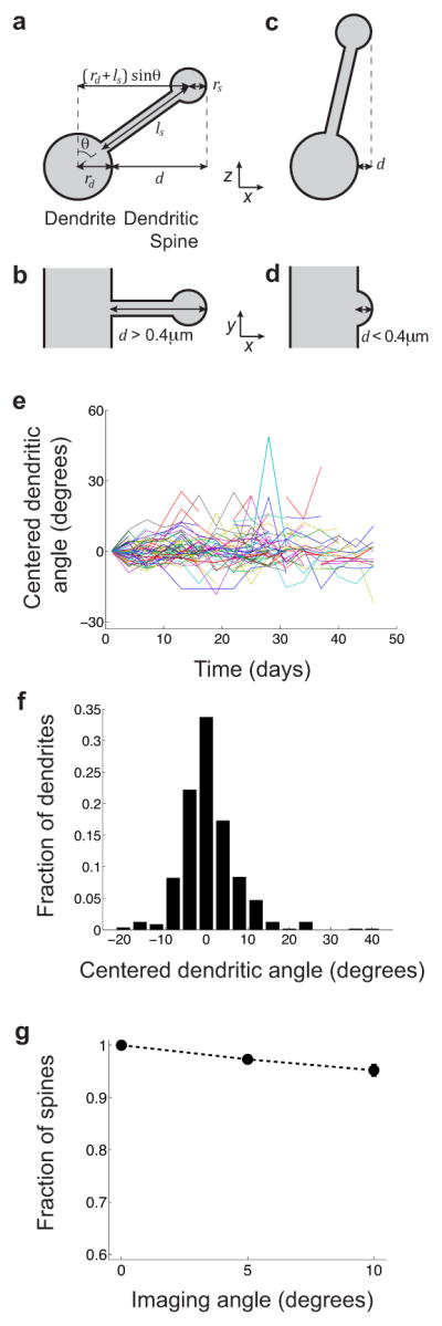
Extended Fig. 6. Variability of imaging angles has virtually no impact on determinations of spine turnover.

We examined empirically whether variations in dendritic angle across different imaging sessions might impact determinations of spine turnover. However, the variations in dendritic angle that were actually present in our datasets were insufficient to cause illusory turnover.

(a, b) Dendritic spines can be detected when the angle (θ) between a spine and the normal vector is large (Supplementary Methods, §IV). View of a dendrite and spine in the (x, z), (a), and optical (x, y), (b), planes.

(c, d) Dendritic spines cannot be detected when the angle between a spine and the normal vector (θ) is small (Supplementary Methods, §IV). View of a dendrite and spine in the (x, z), (c), and optical (x, y), (d), planes.

(e) For every dendrite and time point, we estimated the dendrite’s angle with respect to the optical plane, using the 3D coordinates of two manually labeled points on the dendrite chosen to flank the region of dendrite containing the scored spines. Over time, individual dendrites varied about their initial angle (n = 55 dendrites tracked over 16 sessions; dataset of Fig. 3d).

(f) Distribution of the fluctuations in angle, pooled across the 55 dendrites, relative to the initial angle as seen in the first imaging session. The average magnitude of an angular fluctuation was 4.5°, and 90% of angular fluctuations were <10° in magnitude. Thus, a 5° fluctuation was typical in our dataset, whereas a 10° fluctuation was atypically large.

(g) To determine if variability in the imaging angle might impact determinations of spine turnover, we imaged 18 dendrites in fixed slices while deliberately tilting the imaging plane by 0°, 5° and 10°. We made a total of 989 spine observations. Over 95% of spines scored in the 0°-condition were also correctly scored when the specimen as tilted by 5° or 10°. Overall, the level of angular fluctuations in the in vivo imaging data has virtually no impact on turnover scores.

Extended Fig. 7. Kinetic modeling well describes how optical merging affects spine turnover dynamics as monitored with finite optical resolution.

(a) Diagram of the kinetic scheme used to describe merged spine dynamics (Supplementary Methods, §V). Each state is labeled by the number of actual spines that have merged in appearance to a single spine (a quantity that we call the merged spine order (Supplementary Methods, §III)). State ‘0’ indicates the absence of a spine, and state ‘1’ indicates a spine that is truly unitary. Transitions occur between adjacent states in the kinetic ladder diagram with rate constants r_mn.

(b) The rate constants governing increases in merged spine order depend on two parameters (Supplementary Methods, §V): (i) the initial state or merged spine order; and (ii) the overall degree of merging in the spine image dataset, which is proportional to the product of the spine density and the shortest resolvable inter-spine interval (denoted L) (Supplementary Methods, §III). In contrast, the rate constants governing decreases in merged spine order (inset) depend only on the initial merged spine order (Supplementary Methods, §V).

(c) In the case when all spines are labile, a collapsed kinetic scheme in which a single state (Ψ) combines all merged spine orders above zero approximates the complete model (d) and can be solved mathematically (Supplementary Methods, §V).

(d) The surviving fraction curve generated from the collapsed kinetic scheme (blue curve) fits the empirically observed surviving fraction (black data points) as well as the best-fit model (red).

(e) The asymptotic value of the surviving fraction is a function of the degree of merging (Supplementary Methods, §V). A large degree of merging (as in CA1, blue circle) produces a larger asymptotic value of the merged spine surviving fraction than a small degree of merging (as in neocortex, purple circle).

(f) The estimated lifetime of merged spines is a function of the degree of merging (Supplementary Methods, §V). A large degree of merging (as in the hippocampal CA1, blue circle) produces a longer relative lifetime of merged spines than a small degree of merging (as in the neocortex, purple circle).

Extended Fig. 8. Dynamic spine geometries induce modest levels of apparent spine turnover that cannot explain the turnover measured in vivo.

To study potential effects of fluctuations in spine geometry, we used values for the means and variances of dendrite radius, spine length, and spine radius that were determined by electron microscopy^17,34. We then computationally examined how time-dependent fluctuations in these parameters would affect determinations of spine surviving fraction (Supplementary Methods, §VII).

(a) We examined how fluctuations in dendrite radius, spine radius, spine length and spine angle — individually (colored data points) and all together (black data) — affect the spine surviving fraction when the fluctuating geometric parameters are chosen stochastically in each of two imaging sessions, as a function of the parameter’s time-correlation between the two sessions (Supplementary Methods, §VII). As expected, when the two sessions involved image pairs that were perfectly correlated, the surviving fraction reached 100%. Fluctuations in all four parameters had greater effects than fluctuations in individual geometric parameters.

(b) To estimate the time-dependence of the surviving fraction of scorable spines from (a), we assumed all geometric parameters evolved according to the time-correlation function that we empirically determined from in vivo imaging data (Extended Fig. 9d).

(c) The apparent surviving fraction is the product of the true surviving fraction and the surviving fraction of scorable spines (Supplementary Methods, §VII). For the best-fit kinetic model, the apparent surviving fraction is very close to the true surviving fraction.

(d) The difference between the fitted timescale of the apparent surviving fraction and the true survival timescale is small across the range of model parameters consistent with the in vivo data (Supplementary Methods, §VII).

(e) The graph plots the lower bound of the surviving fraction of scorable merged spines as a function of the time-correlation function shared by all four geometric parameters, for different merged spine orders. As this lower bound increases rapidly with the merged spine order, artifactual turnover due to unscorable spines is unlikely when spine merging is common (Supplementary Methods, §VII).

(f) We combined Fig. 4c and Extended Fig. 8e to bound the turnover that could result from unscorable spines (Supplementary Methods, §VII). As the empirically measured surviving fraction falls below the lower bound obtained for the surviving fraction of scorable merged spines, ongoing changes in the geometric parameters of spines cannot account for the observed spine turnover.

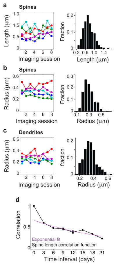
Extended Fig. 9. Dynamics of spine geometries measured in vivo.

(a) Time courses of the spine length, measured from the border of the dendritic shaft to the center of the spine, for five example spines tracked over 8 imaging sessions (left). Distribution of spine lengths (right; N = 344 spine observations).

(b) Time courses of the spine radius, measured from the border to the center of the spine, for five example spines tracked over 8 imaging sessions (left). Distribution of spine radii (right; N = 344 spine observations).

(c) Time courses of the dendritic radius, measured from the border to the center of the dendrite, at the location of five example spines tracked over 8 imaging sessions (left). Distribution of all dendritic radii (right; N = 344 dendrite observations).

(d) Experimental spine length time-correlation function and its exponential fit (Supplementary Methods, §VII).

Extended Fig. 10. Volumes of stable spines fluctuate minimally over time.

To attain an approximate measure of spine volume for stable spines, we quantified each spine’s fluorescence in manually drawn regions-of-interest (ROIs) and normalized it by the fluorescence value in the nearby dendritic shaft, as determined within a ROI of identical shape and size in a single z-section image acquired by two-photon microendoscopy. In addition, each spine’s fluorescence value at each time point is normalized to its own mean over the entire experiment.

(a, b) Mean (± s.e.m.) fluorescence intensities of all spines, (a), and individual spines, (b), from a set of 43 stable spines, across a 21-day-span during which mice (N = 4) were in their home cages (same data as for Fig. 3a). Dashed black line in (a) indicates the mean over all imaging sessions.

(c) The correlation functions of spine radius (green), length (blue), fluorescence (black) and dendritic radius (red) are indistinguishable from each other.

(d) Mean (± s.e.m.) fluorescence intensities of 61 stable spines, across a 46-day-span during which mice (N = 3) initially resided in their home cages (black data points) but later moved to an enriched environment (red points) (same dataset as for Fig. 3d). Dashed black and red lines respectively denote the mean values over the baseline and enriched periods.

References

- 1.Squire LR, Zola-Morgan S. The medial temporal lobe memory system. Science. 1991;253:1380–1386. doi: 10.1126/science.1896849. [DOI] [PubMed] [Google Scholar]
- 2.Frankland PW, Bontempi B. The organization of recent and remote memories. Nat Rev Neurosci. 2005;6:119–130. doi: 10.1038/nrn1607. nrn1607 [pii] [DOI] [PubMed] [Google Scholar]
- 3.Frey U, Morris RG. Synaptic tagging and long-term potentiation. Nature. 1997;385:533–536. doi: 10.1038/385533a0. [DOI] [PubMed] [Google Scholar]
- 4.Barretto RP, et al. Time-lapse imaging of disease progression in deep brain areas using fluorescence microendoscopy. Nat Med. 2011;17:223–228. doi: 10.1038/nm.2292. nm.2292 [pii] [DOI] [PMC free article] [PubMed] [Google Scholar]
- 5.Engert F, Bonhoeffer T. Dendritic spine changes associated with hippocampal long-term synaptic plasticity. Nature. 1999;399:66–70. doi: 10.1038/19978. [DOI] [PubMed] [Google Scholar]
- 6.Maletic-Savatic M, Malinow R, Svoboda K. Rapid dendritic morphogenesis in CA1 hippocampal dendrites induced by synaptic activity. Science. 1999;283:1923–1927. doi: 10.1126/science.283.5409.1923. [DOI] [PubMed] [Google Scholar]
- 7.Holtmaat AJ, et al. Transient and persistent dendritic spines in the neocortex in vivo. Neuron. 2005;45:279–291. doi: 10.1016/j.neuron.2005.01.003. S0896627305000048 [pii] [DOI] [PubMed] [Google Scholar]
- 8.Xu T, et al. Rapid formation and selective stabilization of synapses for enduring motor memories. Nature. 2009;462:915–919. doi: 10.1038/nature08389. nature08389 [pii] [DOI] [PMC free article] [PubMed] [Google Scholar]
- 9.Yang G, Pan F, Gan WB. Stably maintained dendritic spines are associated with lifelong memories. Nature. 2009;462:920–924. doi: 10.1038/nature08577. nature08577 [pii] [DOI] [PMC free article] [PubMed] [Google Scholar]
- 10.Zuo Y, Yang G, Kwon E, Gan WB. Long-term sensory deprivation prevents dendritic spine loss in primary somatosensory cortex. Nature. 2005;436:261–265. doi: 10.1038/nature03715. nature03715 [pii] [DOI] [PubMed] [Google Scholar]
- 11.Yang G, et al. Sleep promotes branch-specific formation of dendritic spines after learning. Science. 2014;344:1173–1178. doi: 10.1126/science.1249098. [DOI] [PMC free article] [PubMed] [Google Scholar]
- 12.Harris KM. Structure, development, and plasticity of dendritic spines. Curr Opin Neurobiol. 1999;9:343–348. doi: 10.1016/s0959-4388(99)80050-6. [DOI] [PubMed] [Google Scholar]
- 13.Mizrahi A, Crowley JC, Shtoyerman E, Katz LC. High-resolution in vivo imaging of hippocampal dendrites and spines. J Neurosci. 2004;24:3147–3151. doi: 10.1523/JNEUROSCI.5218-03.2004. 24/13/3147 [pii] [DOI] [PMC free article] [PubMed] [Google Scholar]
- 14.Barretto RP, Messerschmidt B, Schnitzer MJ. In vivo fluorescence imaging with high-resolution microlenses. Nat Methods. 2009;6:511–512. doi: 10.1038/nmeth.1339. nmeth.1339 [pii] [DOI] [PMC free article] [PubMed] [Google Scholar]
- 15.Gu L, et al. Long-term in vivo imaging of dendritic spines in the hippocampus reveals structural plasticity. J Neurosci. 2014;34:13948–13953. doi: 10.1523/JNEUROSCI.1464-14.2014. 34/42/13948 [pii] [DOI] [PMC free article] [PubMed] [Google Scholar]
- 16.Ziv Y, et al. Long-term dynamics of CA1 hippocampal place codes. Nat Neurosci. 2013;16:264–266. doi: 10.1038/nn.3329. nn.3329 [pii] [DOI] [PMC free article] [PubMed] [Google Scholar]
- 17.Harris KM, Stevens JK. Dendritic spines of CA 1 pyramidal cells in the rat hippocampus: serial electron microscopy with reference to their biophysical characteristics. J Neurosci. 1989;9:2982–2997. doi: 10.1523/JNEUROSCI.09-08-02982.1989. [DOI] [PMC free article] [PubMed] [Google Scholar]
- 18.Moser MB, Trommald M, Andersen P. An increase in dendritic spine density on hippocampal CA1 pyramidal cells following spatial learning in adult rats suggests the formation of new synapses. Proc Natl Acad Sci U S A. 1994;91:12673–12675. doi: 10.1073/pnas.91.26.12673. [DOI] [PMC free article] [PubMed] [Google Scholar]
- 19.Rampon C, et al. Enrichment induces structural changes and recovery from nonspatial memory deficits in CA1 NMDAR1-knockout mice. Nat Neurosci. 2000;3:238–244. doi: 10.1038/72945. [DOI] [PubMed] [Google Scholar]
- 20.Sanders J, Cowansage K, Baumgartel K, Mayford M. Elimination of dendritic spines with long-term memory is specific to active circuits. J Neurosci. 2012;32:12570–12578. doi: 10.1523/JNEUROSCI.1131-12.2012. 32/36/12570 [pii] [DOI] [PMC free article] [PubMed] [Google Scholar]
- 21.Bourne JN, Harris KM. Coordination of size and number of excitatory and inhibitory synapses results in a balanced structural plasticity along mature hippocampal CA1 dendrites during LTP. Hippocampus. 2011;21:354–373. doi: 10.1002/hipo.20768. [DOI] [PMC free article] [PubMed] [Google Scholar]
- 22.Huerta PT, Sun LD, Wilson MA, Tonegawa S. Formation of temporal memory requires NMDA receptors within CA1 pyramidal neurons. Neuron. 2000;25:473–480. doi: 10.1016/s0896-6273(00)80909-5. S0896-6273(00)80909-5 [pii] [DOI] [PubMed] [Google Scholar]
- 23.Yasumatsu N, Matsuzaki M, Miyazaki T, Noguchi J, Kasai H. Principles of long-term dynamics of dendritic spines. J Neurosci. 2008;28:13592–13608. doi: 10.1523/JNEUROSCI.0603-08.2008. 28/50/13592 [pii] [DOI] [PMC free article] [PubMed] [Google Scholar]
- 24.Toni N, Buchs PA, Nikonenko I, Bron CR, Muller D. LTP promotes formation of multiple spine synapses between a single axon terminal and a dendrite. Nature. 1999;402:421–425. doi: 10.1038/46574. [DOI] [PubMed] [Google Scholar]
- 25.Goshen I, et al. Dynamics of retrieval strategies for remote memories. Cell. 2011;147:678–689. doi: 10.1016/j.cell.2011.09.033. S0092-8674(11)01144-5 [pii] [DOI] [PubMed] [Google Scholar]
- 26.Sorra KE, Harris KM. Stability in synapse number and size at 2 hr after long-term potentiation in hippocampal area CA1. J Neurosci. 1998;18:658–671. doi: 10.1523/JNEUROSCI.18-02-00658.1998. [DOI] [PMC free article] [PubMed] [Google Scholar]
- 27.Fusi S, Drew PJ, Abbott LF. Cascade models of synaptically stored memories. Neuron. 2005;45:599–611. doi: 10.1016/j.neuron.2005.02.001. S0896-6273(05)00117-0 [pii] [DOI] [PubMed] [Google Scholar]
- 28.Abraham WC, Robins A. Memory retention--the synaptic stability versus plasticity dilemma. Trends Neurosci. 2005;28:73–78. doi: 10.1016/j.tins.2004.12.003. S0166-2236(04)00370-4 [pii] [DOI] [PubMed] [Google Scholar]
- 29.Wu XE, Mel BW. Capacity-enhancing synaptic learning rules in a medial temporal lobe online learning model. Neuron. 2009;62:31–41. doi: 10.1016/j.neuron.2009.02.021. S0896-6273(09)00167-6 [pii] [DOI] [PMC free article] [PubMed] [Google Scholar]
- 30.Poirazi P, Mel BW. Impact of active dendrites and structural plasticity on the memory capacity of neural tissue. Neuron. 2001;29:779–796. doi: 10.1016/s0896-6273(01)00252-5. S0896-6273(01)00252-5 [pii] [DOI] [PubMed] [Google Scholar]
- 31.Feng G, et al. Imaging neuronal subsets in transgenic mice expressing multiple spectral variants of GFP. Neuron. 2000;28:41–51. doi: 10.1016/s0896-6273(00)00084-2. S0896-6273(00)00084-2 [pii] [DOI] [PubMed] [Google Scholar]
- 32.Holtmaat A, et al. Long-term, high-resolution imaging in the mouse neocortex through a chronic cranial window. Nat Protoc. 2009;4:1128–1144. doi: 10.1038/nprot.2009.89. nprot.2009.89 [pii] [DOI] [PMC free article] [PubMed] [Google Scholar]
- 33.Dombeck DA, Harvey CD, Tian L, Looger LL, Tank DW. Functional imaging of hippocampal place cells at cellular resolution during virtual navigation. Nat Neurosci. 2010;13:1433–1440. doi: 10.1038/nn.2648. nn.2648 [pii] [DOI] [PMC free article] [PubMed] [Google Scholar]
- 34.Mishchenko Y, et al. Ultrastructural analysis of hippocampal neuropil from the connectomics perspective. Neuron. 2010;67:1009–1020. doi: 10.1016/j.neuron.2010.08.014. S0896-6273(10)00624-0 [pii] [DOI] [PMC free article] [PubMed] [Google Scholar]