Abstract.
As the panoramic x-ray is the most common extraoral radiography in dentistry, segmentation of its anatomical structures facilitates diagnosis and registration of dental records. This study presents a fast and accurate method for automatic segmentation of mandible in panoramic x-rays. In the proposed four-step algorithm, a superior border is extracted through horizontal integral projections. A modified Canny edge detector accompanied by morphological operators extracts the inferior border of the mandible body. The exterior borders of ramuses are extracted through a contour tracing method based on the average model of mandible. The best-matched template is fetched from the atlas of mandibles to complete the contour of left and right processes. The algorithm was tested on a set of 95 panoramic x-rays. Evaluating the results against manual segmentations of three expert dentists showed that the method is robust. It achieved an average performance of in Dice similarity, specificity, and sensitivity.
Keywords: medical image, automatic segmentation, statistical modeling, panoramic x-ray, mandible
1. Introduction
Since digital radiography has found its way into dentistry, many new applications for processing medical images have been proposed, including dental image registration, lesion detection, bone healing analysis, diagnosis of osteoporosis, and dental forensics.
Automatic detection of maxillofacial landmarks in lateral cephalometric radiography has recently attracted some attention;1,2 whereas other researchers focused on panoramic x-rays (i.e., orthopantomogram) and introduced methods for their registration to give clinicians the complementary information provided by different modalities,3 extracted the region of interest of each tooth by means of vertical and horizontal integral projections,4 or presented methods for detection of carotid artery calcification.5
Segmentation of anatomical structures is a vital step for many applications. No reliable general algorithm has been proposed for medical image segmentation due to shape irregularities, normal variations, and poor image modalities (such as low contrast, uneven exposure, noise, and various image artifacts). In these circumstances, prior shape knowledge and a presegmented atlas of templates can result in a more accurate boundary detection. Many generative models have been proposed for medical image segmentation given a training set of images and corresponding label maps.6–8 Tooth segmentation and forming an “automated dental identification system” for forensic odontology9–16 have also gained some attention in the past decade. Jain and Chen10 were the first to propose a semiautomatic probabilistic method for tooth segmentation and contour matching in bitewing images based on integral projections. They used the Bayes rule and radial scan to extract the tooth contour, while initially separating each tooth from the opposite and adjacent teeth by means of integral projections.
Currently, panoramic radiography is the most common extraoral technique in today’s dentistry as a result of its low cost, simplicity, informative content, and the reduced exposure of the patient. Because this radiography technique provides the dentist with an overall view of the alveolar process, condyles, sinuses, and teeth, it plays a major role in diagnosis of dental caries, jaw fractures, systemic bone diseases, unerupted teeth, and intraosseous lesions. Hereby, an automatic method for segmentation of mandible in panoramic x-ray based on prior knowledge of its shape and manually segmented templates is proposed. To the best of our knowledge, this is the first effort ever made to segment mandible bone in a panoramic dental x-ray, and its outcomes can affect many applications, including, but not limited to, panoramic image registration, forensic odontology, dental biometrics, intraosseous lesion detection, and analysis of other problems, such as dental caries, in panoramic x-rays.
The remainder of this paper is organized as follows. Section 2 covers the materials and methods. Section 2.1 explains the dataset gathered for this research, whereas the details of the proposed algorithm are discussed in Sec. 2.2. Experimental results are provided in Sec. 3, and the conclusion and plans for future works are presented in Sec. 4.
2. Materials and Methods
2.1. Prepared Dataset
The original dataset used in this study composed of almost 2000 digital panoramic x-rays in BMP format of pixels taken by the Soredex CranexD digital panoramic x-ray unit. All the images were taken for diagnostic purposes and treatment planning and no radiography record was taken for the purpose of this study. Two subsets were selected from the original set, but prior to selection, some exclusion criteria were applied to narrow down the sample size. Records with implants were excluded. Also, to ensure that no deciduous tooth was present in the images, and that the growth of jaw had almost completed, patients below 20 years of age were excluded from the dataset. Low-quality x-rays, which were blurred or malposed due to technician’s error or patient’s lack of cooperation, were also excluded from the dataset.
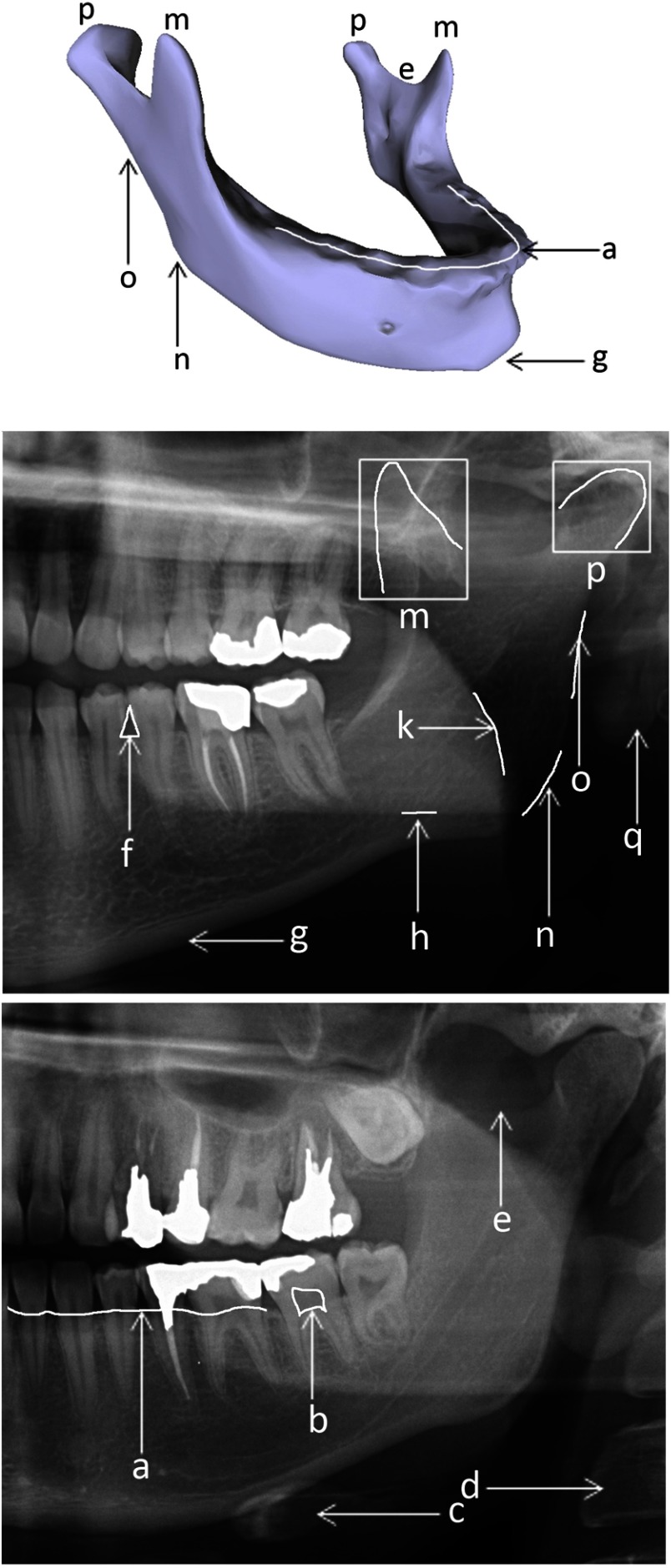
For the first subset, a maxillofacial radiologist sorted out the panoramic x-rays based on several qualitative features such as width of ramuses, vertical distance between alveolar process and inferior border of mandible, acuteness of gonial angle [Fig. 2(n)], overall convexity of inferior border [Fig. 2(g)], whether there was a concavity around the gonial angle, shape of coronoid process [Fig. 2(m)], shape of condyles [Fig. 2(p)], and depth of sigmoid notch [Fig. 2(e)]. She then purposefully selected 116 images to cover all varieties of mandible shapes seen on panoramic x-rays regarding these criteria. These images were considered templates of the atlas.
Fig. 2.
Landmarks of mandible bone (top image) and panoramic x-rays: (a) superior border of alveolar process, (b) dental pulp, (c) hyoid bone, (d) vertebra, (e) sigmoid notch, (f) interdental papilla, (g) inferior border of mandible, (h) shadow of inferior border of the opposite side of mandible, (k) shadow of dorsal border of tongue, (m) coronoid process, (n) gonial angle, (o) exterior border of ramus, (p) condyle/condylar process, (q) shadow of earlobe.
For the second subset, 30 images were chosen randomly from the same large dataset and grouped as the statistical set through which the parameters of the system were assigned.
The mandibles of all 146 images were manually segmented by three expert dentists working at Shahid Beheshti University of Medical Sciences, Tehran. In order to generate a reliable unified ground truth for each x-ray, a voting policy was used. According to this voting policy, a pixel belonged to the object (mandible) if at least two of the three manual segmentations defined that pixel as object (Fig. 1).
Fig. 1.
Generating the unified ground truth: (a) manual segmentations of three experts and (b) unified ground truth based on the voting policy.
2.2. Proposed Method
In order to thoroughly understand the details of the proposed method, it is encouraged to first acquire a general knowledge on the anatomy of mandible bone. Figure 2 depicts this bone and a portion of two panoramic x-rays explaining important landmarks, shadows, and illusions, which affect the automatic segmentation of mandible in various ways.
Based on the anatomy of the mandible bone (Fig. 2), its boundary can be divided into four subregions: (1) superior border of alveolar process [Fig. 2(a)], (2) inferior border of mandible [Fig. 2(g)], (3) exterior border of ramus [Fig. 2(o)], and (4) processes of mandible [Fig. 2(p) and Fig. 2(m)]. Consequently, a four-step segmentation algorithm was proposed. In each step of this algorithm, a subregion of mandible contour was extracted through a specially designed method based on the prior knowledge of the subregion’s shape.
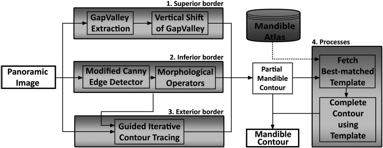
Figure 3 illustrates the four steps of the proposed method. In the first step, the gap between the upper and lower teeth and consequently superior border of the alveolar process was detected through integral projections. Second, the edge representing the inferior boundary of mandible was extracted, which came into use as a starting point for the contour tracing algorithm in step three, which extracted the exterior boundaries of the left and right ramuses. During the fourth and final step, the best-matched mandible template was fetched from the atlas and its condyles and coronoid processes were used to estimate the boundary of these sub-substructures.
Fig. 3.
Block diagram of the proposed segmentation method.
The limit points connecting the four subregions of mandible were estimated through the statistical set prior to segmentation of the query image. To form this estimation, the end points of each subregion were manually marked on statistical samples and their widths and heights were calculated and averaged with respect to the widths and heights of their corresponding images. This estimation played two major roles in the segmentation algorithm: to declare the proportional width where the inferior border of mandible ended, which stated the end of step 2, and to declare the proportional height where the exterior border of ramus ended, which stated the end of step 3.
Images were all preprocessed to remove overlaid device labels and were downsampled by a factor of 8 ( pixels) to lower the computational cost. A small median filter was applied to resolve salt and pepper noise. Panoramic radiographies also suffer from uneven exposure resulting in an inhomogeneous contrast along the x-ray. Based on the results of Ref. 17, the “contrast-limited adaptive histogram equalization” (CLAHE) technique was applied, which divides the x-ray into smaller tiles, increases the local contrast of each tile, and finally merges them using a bilinear interpolation. CLAHE emphasizes the edges in each tile but does not intensify the noise in homogenous areas by putting a limit on the contrast increase.17
2.2.1. Superior border of alveolar process
The proposed algorithm for separating upper and lower teeth was based on the work by Jain and Chen10 on an intraoral radiograph known as the bitewing. In both bitewing and panoramic x-rays, patient bites on a mouthpiece while images of upper and lower teeth are projected on the film. Therefore, the gap between upper and lower teeth is presented as a lucent (dark) horizontal strip in these images, which, following the original study, we refer to it as the “gap valley” (GV).
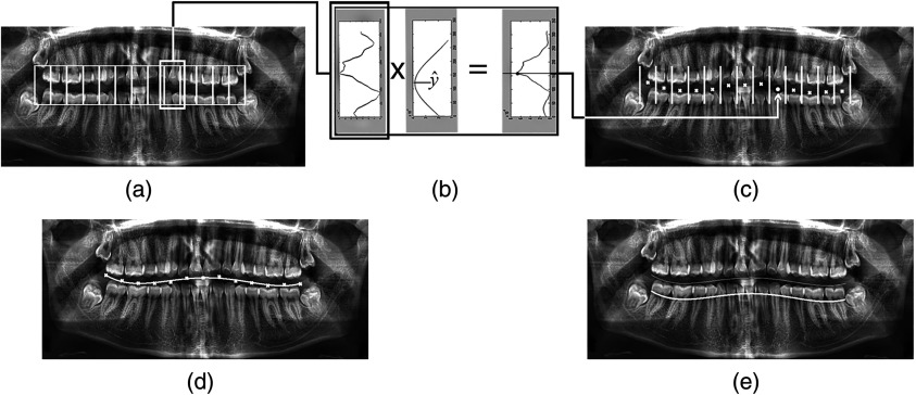
The area that most definitely contained the GV was estimated using the images of the statistical set. As shown in Fig. 4(a), this area was divided into vertical strips, each equal to the estimated width of a tooth in panoramic radiography. Extraction of the GV was based on two facts: the lucent space between the upper and lower teeth is expected to have the lowest horizontal integral projection among its neighbors, and the shape of the GV does not go through rapid changes during its course among adjacent teeth.
Fig. 4.
Extracting superior border of alveolar process: (a) the area containing the gap valley is divided into vertical strips; (b and c) in each strip, maximum of the horizontal integral projection function multiplied by gap valley (GV) prediction Gaussian function corresponds to the GV point of that strip; (d) a fourth-degree polynomial curve is fitted to the acquired GV points; and (e) GV curve is shifted downward to match the superior border of the alveolar process.
In each vertical strip, if is the predicted height of the GV and are the local minima of the horizontal integral projection function,10 the probability of a local minima with height being the GV can be estimated through the following probability function:
| (1) |
| (2) |
| (3) |
In Eq. (2), is a normalizing constant to ensure that sums up to 1, and is the likelihood of the gap lying in the local minima (), while the integral projection of its pixel intensities equals . In Eq. (3), is a Gaussian function with the mean parameter set to .
The algorithm was initiated from the middle strip and continued toward the adjacent left and right strips. In each strip, the local minimum () with the highest probability was selected as the position of the GV point [Fig. 4(b)]. The prediction value for the middle strip was assigned to the midpoint of the strip, and it got its value from the previously calculated position of the GV point for the adjacent strips. This procedure adjusted and fixed the height of each GV point relative to its adjacent strip and ensured that the GV followed a smooth path.
In the end, a fourth-degree polynomial curve was fit to the GV points through regression to match the natural anteroposterior curve of Spee on each side of the human dental occlusion. Figure 4(c) shows the calculated GV points of all vertical strips, and Fig. 4(d) illustrates the curve fit to these points. The left and right limit points of the curve were based on the estimation made through the statistical set, which indicated that teeth were approximately located horizontally in the medial 0.62 portion of the image.
As shown in Fig. 4(e), the GV curve needed to be shifted downward and set to the “cementoenamel junction” (CEJ) of the lower teeth where the crown and root meet, which, in a healthy bone, is a good estimate of the superior border of the alveolar process [Fig. 2(a)]. Due to the following four factors, the neck area (CEJ) is more lucent compared to its higher and lower regions in panoramic x-ray: (1) lucent interdental papillas [triangular lucent areas between adjacent teeth, see Fig. 2(f)]; (2) lucent dental pulps [Fig. 2(b)]; (3) lack of enamel (as opposed to the crown); and (4) lack of surrounding bone (as opposed to the root). By transferring the GV curve downward and summing the intensity of the pixels lying upon it, it was expected that the global minimum of the summation function would match the superior border of the alveolar process.
2.2.2. Inferior border of mandible
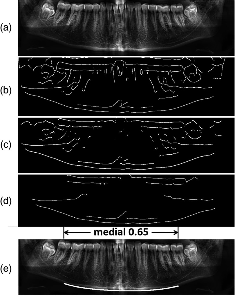
The inferior border of mandible is a condensed structure and appears as a fine horizontal edge at the bottom of the panoramic x-ray [Figs. 2(g) and 5(a)]. To extract this horizontal edge, a modified version of the Canny edge detector was created with the horizontal variance of its Gaussian filter twice its vertical variance. Such a filter weakened the vertical edges while preserving the horizontal ones, which resulted in a binary edge-map with more horizontal edges [Fig. 5(b)]. The edge-map was then convolved with a horizontal Prewitt filter, which removed all the vertical edges, as shown in Fig. 5(c).
Fig. 5.
Extracting inferior border of mandible: (a) original image, (b) after applying modified Canny edge detector, (c) after applying horizontal Prewitt operator, (d) after removal of small connected components, and (e) the extracted inferior border of mandible.
Radiography is the projection of a 3-dimensional object on 2-dimensional film, and as a result, it suffers from the superimposition of the anatomical structures. In panoramic imagery, this factor is heightened due to the rotation of the x-ray tube around the patient’s head, resulting in shadows and ghost objects all over the image. The hyoid bone, which is an isolated bone located below the tongue and above the thyroid cartilage, is one of these structures commonly superimposed on or below the inferior border of the mandible [Fig. 2(c)]. To remove such unwanted small edges, a flood-fill area opening algorithm was performed on the binary edge-map to remove the small connected components, such as remnants of the hyoid bone. Figure 5(d) illustrates the final edge-map of the panoramic x-ray after performing the described morphological operators.
The lowest horizontal edge on the final edge-map corresponds to the inferior border of the mandible. As mentioned earlier in Sec. 2.2, the left and right limits of this substructure were primarily estimated through the statistical set; therefore, the middle portion of the edge located horizontally inside the medial 0.65 portion of the image was extracted as the inferior border [Fig. 5(e)].
2.2.3. Exterior borders of ramuses
The inferior border of mandible is connected to the exterior border of ramus through the gonial angle, which is a curved and usually weak edge [Fig. 2(n)]. Irregular shape of the gonial angle and superimposition of structures, such as vertebrae [Fig. 2(d)], earlobe [Fig. 2(q)], inferior border of the opposite side of the mandible [Fig. 2(h)], and dorsal surface of the tongue [Fig. 2(k)], make the extraction of the exterior border of the ramus a challenging procedure. Although these shadows and superimpositions were not present in all panoramic images due to variations of human anatomy and different head poses of patients during radiography, they need to be taken into account for a general segmentation method.
In order to overcome these obstacles, a guided contour tracing method based on the average shape model of the mandible was proposed. In this method, two directional contour tracing tasks started from the left and right endpoints of the inferior border of the mandible (extracted in Sec. 2.2.2) and continued toward the condyles of both sides [Fig. 2(p)]. In each step of this iterative procedure, the neighbor pixel with the strongest edge magnitude was chosen as the next pixel on the contour.
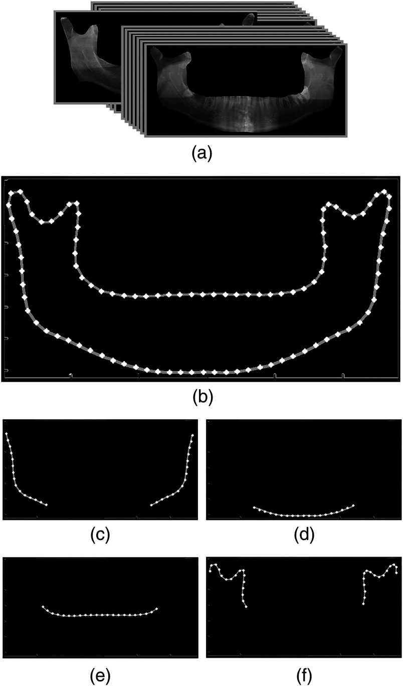
To model the average shape, the statistical set, which consisted of 30 manually segmented mandibles, was used [Fig. 6(a)]. The same number of landmark points was chosen on contours of manually segmented mandibles. In order to do so, subregions of mandible were separated and a specific number of equally spaced landmarks were chosen on each subcontour. As a result, there existed a one-to-one mapping between the landmark points of all the models. Models were then aligned through minimizing the sum of squares of distances between equivalent points by means of the Procrustes method.18,19 The mean position for each landmark point on the contour was calculated by averaging the position of 30 aligned samples for that point. As shown in Fig. 6(b), the average shape model was finally created by connecting the calculated average landmarks. Figures 6(c)–6(f) present the average shape model of each subregion separately. The average shape model of the exterior border of mandible [Fig. 6(c)] was used in the contour tracing algorithm.
Fig. 6.
Generating the average shape model of mandible: (a) manually segmented images of the statistical set, (b) average shape model, (c–f) separated average shape models of subregions.
The proposed contour tracing algorithm used the difference between the image gradient direction () and the gradient of the average shape model of the exterior border of mandible () as a criterion to amplify or weaken the magnitude of the image gradient (). The modified gradient magnitude () was calculated as follows:
| (4) |
| (5) |
where is a normalizing constant and is the gradient magnitude on each pixel. In Eq. (5), smaller values of correspond to edges, which lie in the same direction as the exterior border of the average shape model. In the modified gradient map (), the magnitude of edges that lie in the correct direction are intensified and the probability of them being chosen in the next iteration of contour tracing is increased.
A model dissimilarity threshold () was also defined, which prevented the contour tracing procedure from getting sidetracked and continuing on a wrong path. In other words, the contour tracing could only continue in a direction that lay in the threshold, where was the average shape model gradient at pixel ; otherwise, the procedure had to go some iterations back and choose the next best edge with the highest probability.
The guided iterative contour tracing method followed the exterior borders of the left and right ramuses until it reached the height of the condyles of both sides, which is estimated through the statistical set to be , where is the height of the query image.
2.2.4. Processes of mandible
There is a condyloid process [Fig. 2(p)] and a coronoid process [Fig. 2(m)] on each side of the mandible bone. The condyloid process (condyle) is located inside the glenoid fossa and is surrounded by bony structures. As such, it does not have an apparent boundary in most panoramic x-rays. Besides, as shown in Fig. 2, the condyloid and coronoid processes are superimposed by vertebra, maxilla (upper jaw), and in some cases by the impacted upper wisdom teeth. The weak edges and the steep sigmoid notch, which connect these two processes [Fig. 2(e)], make it more difficult to automatically segment these structures.
An atlas-based segmentation method was proposed for this step, which used manually segmented mandibles as templates to complete the contour of the processes. To construct the atlas, a specialized doctor in maxillofacial radiology selected 116 panoramic x-rays to cover all the varieties of mandible shapes in this radiography technique. Because the case selection was carried out in a manner to fulfill this purpose, we designated each segmented image in the atlas as a single template.
The boundaries of all templates were partitioned into the four subcontours (i.e., superior border of alveolar process, inferior border of mandible, exterior borders of ramuses, and the processes), and a specified number of equally spaced landmark points was automatically marked on each subcontour, as in Sec. 2.2.3. The three previously extracted subcontours of the query image (i.e., superior border of alveolar process, inferior border of mandible, and exterior borders of ramuses) went through a similar procedure and had the same number of equally spaced landmark points automatically marked upon them. Finally, in order to complete the segmentation of the query image, atlas was searched to find the best-matched template based on the least sum of squares of distances between equivalent landmark points of the three subcontours.
Matching templates with the query image was accomplished by means of the Procrustes analysis,18 which tries to minimize the sum of squares of distances between two sets of equivalent points through translation, rotation, and scaling of one set of points.20 The template whose points are mapped to the landmark points of the query image with the least sum of square of distances is chosen as the best-matched template.
When the best-matched template was aligned on the query image using the Procrustes method, the landmark points located on the processes subcontour were projected onto the query image as an estimate for the boundaries of the condyles and coronoid processes. Segmentation of the last subregion was completed by limited shifting of these newly positioned landmarks in a direction perpendicular to the contour in search of the strongest neighbor edge.19
It is worth noting that contour tracing for the exterior borders of the ramuses started from the endpoints of the inferior border of the mandible. Also, due to the translation, rotation, and, more importantly, scaling performed by the Procrustes method, the endpoints of the processes were matched to the upper endpoints of the exterior border of the ramuses, and they were also almost matched to the endpoints of the superior border of the alveolar process. Therefore, because the endpoints of each subcontour were matched to the endpoints of the adjacent subcontour, no final merging of the contours was required.
3. Experimental Results
In this section, the results of testing experiments carried out to verify the performance of the automatic mandible segmentation method are reported. The results are all based on the MATLAB implementation of the algorithm, which made use of the image processing toolbox. The algorithm ran on a standard PC (Intel Core i7, 2.30 GHz, 6 GB RAM, 64-bit OS) and was able to segment the downsampled panoramic x-rays in an average time of , with no means of parallel computing.
All the samples were segmented by three expert dentists, and the results of their segmentations were unified based on the voting policy explained in Sec. 2.1. Among the 116 cases that formed the atlas, there were 21 patients who were completely toothless or had long toothless areas in both jaws. These images were excluded from validation, and the proposed algorithm was tested only on the remaining 95 panoramic x-rays. Because these 95 images were also included in creating the atlas of mandibles, the testing was carried out in a leave-one-out fashion. In other words, when the algorithm searched the atlas for the best-matched template to complete the segmentation in Sec. 2.2.4, the template created using the same panoramic x-ray would not be fetched.
For every case, segmentation performance was evaluated against the unified gold-standard manual segmentation. For this matter, three overlap measures known as Dice similarity coefficient (DSC), specificity, and sensitivity were computed according to the true positive (TP), true negative (TN), false positive (FP), and false negative (FN) values.21 DSC was computed as , specificity was computed as , and sensitivity was computed as .
We also carried out contour-based distance measures to evaluate the segmentation performance of each subregion separately. Hausdorff distance (HD) was used to measure the maximum distance (in pixels) between the boundaries of corresponding subregions of the two contour sets, i.e., automatic segmentation and gold standard. If and are the two contours, HD is defined as
| (6) |
| (7) |
where is the Euclidean distance between the and pixels. Comparing the HD values of different subregions informs us of the performance of each segmentation technique. Due to variable distortion and magnification in panoramic x-rays, the HD is reported in pixels rather than millimeters.
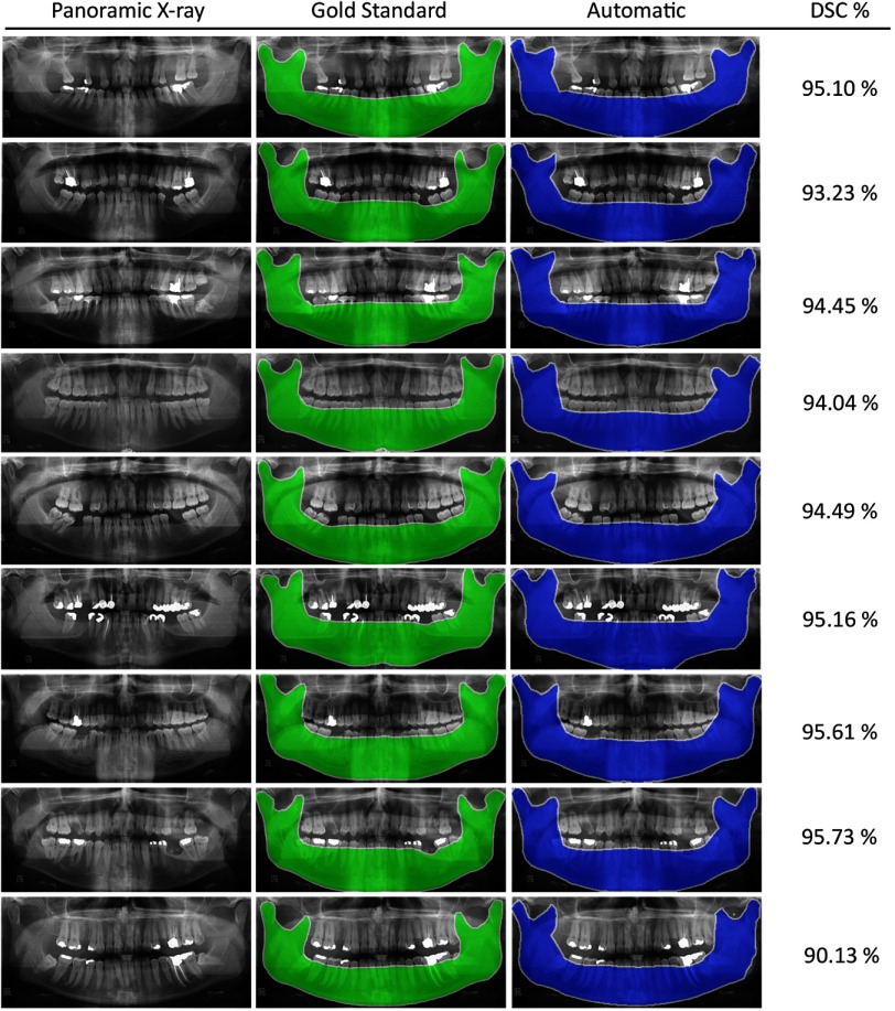
Tables 1 and 2 summarize the evaluation metrics obtained from testing the proposed algorithm on 95 panoramic images. The mean and standard deviation of the metrics are reported to demonstrate accuracy and precision of the proposed automatic segmentation method. Figure 7 depicts outputs of the automatic and manual mandible segmentations in some panoramic x-rays.
Table 1.
Evaluation results of mandible segmentation compared to gold standard.
| Criteria | Mean (%) |
|---|---|
| DSC | |
| Specificity | |
| Sensitivity |
Note: DSC, Dice similarity coefficient.
Table 2.
Evaluation results of Hausdorff distance compared to gold standard.
| Subregion | Mean (pixels) |
|---|---|
| Superior border | |
| Inferior border | |
| Exterior border | |
| Processes |
Fig. 7.
Experimental results of the automatic segmentation method in comparison with the manually segmented gold standards, along with their Dice similarity coefficient (DSC) values.
The manual segmentations of each of the three experts were also compared against the gold standard and evaluated using the same metrics. The results show that manual segmentations of experts have an average specificity of , sensitivity of , and DSC of .
4. Conclusion and Discussion
An efficient, fast, and robust four-step method was proposed for automatic segmentation of mandible in panoramic x-rays without any operator input. To the best of our knowledge, this manuscript presents the first research carried out on segmentation of mandible bone in panoramic radiography. The algorithm was tested on 95 images, which were manually segmented by three expert dentists, and results were compared through supervised criteria, such as DSC, sensitivity, specificity, and HD.
Based on the statistics reported in Table 2 and as is evident in Fig. 7, the condylar and coronoid processes are prone to the most segmentation errors. These areas are superimposed by adjacent bony structures and maxillary sinuses, resulting in hardly noticeable edges. Analyzing the manual segmentations of dentists also confirmed that even the experts’ segmentations did not conform in the processes subregion. Fortunately, these areas contain no substantial information in panoramic radiography. However, comparing the average performance of automatic segmentation with performances of individual experts—all of which were calculated to be above 98%—reveals that the automatic method can still be improved to match the gold standard more closely.
The proposed method is fast and also robust to image artifacts and inhomogeneous contrast of panoramic x-rays, but it may generate false results for cases with large toothless areas in which the GV is not a narrow lucent strip but a wide and vast toothless area, which cannot be detected through horizontal integral projections.
The closest study to the current one was carried out by Frejlichowski and Wanat,4 in which they segmented dental panoramic x-rays into regions, each containing a single tooth. It needs to be noted that the proposed method suffered from some theoretical shortcomings regarding the removal of areas below the roots of the teeth, where they translated the curve separating the upper and lower jaws vertically in search of an alignment, where the sum of pixels it passed through was lower than the surrounding results. In fact, there is no supporting evidence that the sum of intensities of pixels below the roots of teeth is smaller than that of its adjacent areas.
Results of the current study seem promising and can lead to further investigations in the field of automatic segmentation of structures in different head and neck radiography techniques. The output of this study can be used in various scenarios, such as improving registrations of panoramic x-rays through the information gained from a segmented mandible.3 It can affect dental biometrics, which has become a popular field of research. It is also a promising method for human identification.10,11,15,16
Intraosseous lesions of the mandible can be detected by performing pattern recognition on the mandible body, which is extracted through the proposed method. Because panoramic radiography is by far the most utilized form of paraclinical record in today’s dentistry (and not all dentists are experienced enough to detect intraosseous lesions), designing a system for autonomous detection of these damaged tissues seems like a good practice that could also result in early detection of lesions. The proposed method can be further extended to detect anatomic landmarks. As such, detecting locations of dental work in panoramic x-rays can be of great use, mostly in cases of dental forensics and detection of periapical lesions.
Biographies
Amir Hossein Abdi simultaneously studied dentistry and computer engineering at Shahid Beheshti University and graduated from both in 2011. He received his MSc degree from Sharif University of Technology in 2013. He was then elected as the chairman of league in the national Robocup committee of Iran for two years. He is currently a PhD candidate at the University of British Columbia, and his main research interests are biomedical image processing and 3-D biomechanical modeling.
Shohreh Kasaei is a professor at Sharif University of Technology. She received her PhD degree from Queensland University of Technology, Australia. She was awarded best graduate engineering student by University of the Ryukyus in 1994, the best overseas PhD student by the Ministry of Science, Research, and Technology of Iran, and a distinguished researcher at Sharif University of Technology in 2002 and 2010. She has published more than 30 journal papers.
Mojdeh Mehdizadeh received her DDS and specialized doctorate in maxillofacial radiology from Isfahan University of Medical Sciences, Iran, in 1994 and 1997, respectively. She has been teaching in the department of maxillofacial radiology of this university as an associate professor since 2009. She has been a member of International Dento Maxillofacial Radiology (IDMFR) and the European Society of Head and Neck Radiology (ESHNR) since 2006.
References
- 1.Rueda S., Alcaniz M., “An approach for the automatic cephalometric landmark detection using mathematical morphology and active appearance models,” Med. Image Comput. Comput. Assist. Interv. 9, 159–166 (2006). 10.1007/11866565_20 [DOI] [PubMed] [Google Scholar]
- 2.Mondal T., Jain A., Sardana H. K., “Automatic craniofacial structure detection on cephalometric images,” IEEE Trans. Image Process. 20(9), 2606–2614 (2011). 10.1109/TIP.2011.2131662 [DOI] [PubMed] [Google Scholar]
- 3.Mekky N. E., Abou-Chadi F. E., Kishk S., “A new dental panoramic x-ray image registration technique using hybrid and hierarchical strategies,” in Int. Conf. on Computer Engineering and Systems (ICCES), pp. 361–367 (2010). 10.1109/ICCES.2010.5674886 [DOI] [Google Scholar]
- 4.Frejlichowski D., Wanat R., “Automatic segmentation of digital orthopantomograms for forensic human identification,” in Image Analysis and Processing (ICIAP) 2011, pp. 294–302, Springer Berlin Heidelberg; (2011). 10.1007/978-3-642-24088-1_31 [DOI] [Google Scholar]
- 5.Sawagashira T., et al. , “An automatic detection method for carotid artery calcifications using top-hat filter on dental panoramic radiographs,” in Annual Int. Conf. of the IEEE Engineering in Medicine and Biology Society, EMBC, pp. 6208–6211 (2011). 10.1109/IEMBS.2011.6091533 [DOI] [PubMed] [Google Scholar]
- 6.Sabuncu M. R., et al. , “A generative model for image segmentation based on label fusion,” IEEE Trans Med Imaging 29(10), 1714–1729 (2010). 10.1109/TMI.2010.2050897 [DOI] [PMC free article] [PubMed] [Google Scholar]
- 7.Pohl K. M., et al. , “A Bayesian model for joint segmentation and registration,” Neuroimage 31(1), 228–239 (2006). 10.1016/j.neuroimage.2005.11.044 [DOI] [PubMed] [Google Scholar]
- 8.Ashburner J., Friston K. J., “Unified segmentation,” Neuroimage 26(3), 839–851 (2005). 10.1016/j.neuroimage.2005.02.018 [DOI] [PubMed] [Google Scholar]
- 9.Fahmy G., et al. , “Toward an automated dental identification system,” J. Electron. Imaging 14(4), 043018 (2005). 10.1117/1.2135310 [DOI] [Google Scholar]
- 10.Jain A. K., Chen H., “Matching of dental X-ray images for human identification,” Pattern Recognit. 37(7), 1519–1532 (2004). 10.1016/j.patcog.2003.12.016 [DOI] [Google Scholar]
- 11.Lin P. L., Lai Y. H., Huang P. W., “An effective classification and numbering system for dental bitewing radiographs using teeth region and contour information,” Pattern Recognit. 43(4), 1380–1392 (2010). 10.1016/j.patcog.2009.10.005 [DOI] [Google Scholar]
- 12.Lin P. L., Lai Y. H., Huang P. W., “Dental biometrics: human identification based on teeth and dental works in bitewing radiographs,” Pattern Recognit. 45(3), 934–946 (2012). 10.1016/j.patcog.2011.08.027 [DOI] [Google Scholar]
- 13.Mahoor M. H., Abdel-Mottaleb M., “Classification and numbering of teeth in dental bitewing images,” Pattern Recognit. 38(4), 577–586 (2005). 10.1016/j.patcog.2004.08.012 [DOI] [Google Scholar]
- 14.Nassar D. E. M., Ammar H. H., “A neural network system for matching dental radiographs,” Pattern Recognit. 40(1), 65–79 (2007). 10.1016/j.patcog.2006.04.046 [DOI] [Google Scholar]
- 15.Nomir O., Abdel-Mottaleb M., “A system for human identification from X-ray dental radiographs,” Pattern Recognit. 38(8), 1295–1305 (2005). 10.1016/j.patcog.2004.12.010 [DOI] [Google Scholar]
- 16.Zhou J., Abdel-Mottaleb M., “A content-based system for human identification based on bitewing dental X-ray images,” Pattern Recognit. 38(11), 2132–2142 (2005). 10.1016/j.patcog.2005.01.011 [DOI] [Google Scholar]
- 17.Suprijanto S., et al. , “Image contrast enhancement for film-based dental panoramic radiography,” in Int. Conf. on System Engineering and Technology (ICSET), pp. 1–5 (2012). 10.1109/ICSEngT.2012.6339321 [DOI] [Google Scholar]
- 18.Gower J. C., “Generalized Procrustes analysis,” Psychometrika 40(1), 33–51 (1975). 10.1007/BF02291478 [DOI] [Google Scholar]
- 19.Cootes T. F., et al. , “Active shape models-their training and application,” Comput. Vis. Image Underst. 61(1), 38–59 (1995). 10.1006/cviu.1995.1004 [DOI] [Google Scholar]
- 20.Schonemann P. H., “A generalized solution of the orthogonal Procrustes problem,” Psychometrika 31(1), 1–10 (1966). 10.1007/BF02289451 [DOI] [Google Scholar]
- 21.Dice L. R., “Measures of the amount of ecologic association between species,” Ecology 26(3), 297–302 (1945). 10.2307/1932409 [DOI] [Google Scholar]


