LoopIng: a template-based tool for predicting the structure of protein loops

Abstract

Motivation: Predicting the structure of protein loops is very challenging, mainly because they are not necessarily subject to strong evolutionary pressure. This implies that, unlike the rest of the protein, standard homology modeling techniques are not very effective in modeling their structure. However, loops are often involved in protein function, hence inferring their structure is important for predicting protein structure as well as function.

Results: We describe a method, LoopIng, based on the Random Forest automated learning technique, which, given a target loop, selects a structural template for it from a database of loop candidates. Compared to the most recently available methods, LoopIng is able to achieve similar accuracy for short loops (4–10 residues) and significant enhancements for long loops (11–20 residues). The quality of the predictions is robust to errors that unavoidably affect the stem regions when these are modeled. The method returns a confidence score for the predicted template loops and has the advantage of being very fast (on average: 1 min/loop).

Availability and implementation: www.biocomputing.it/looping

Contact: anna.tramontano@uniroma1.it

Supplementary information: Supplementary data are available at Bioinformatics online.

1 Introduction

The functional characterization of proteins is an important and, at the same time, challenging problem in biology. The annotation task can be facilitated by the knowledge of the three-dimensional (3D) structure of the protein of interest and of its complexes (Holtby et al., 2013). However, determining a protein 3D structure experimentally is an expensive and time-consuming task. As a result, the number of experimentally solved protein structures is very small compared to the number of available protein sequences. However, this situation is changing and homology modeling is currently making structural information available for a large number of proteins (Schwede, 2013). Structurally speaking, proteins consist of elements of secondary structure (alpha helices and beta strands) connected by loops. These often play important functional roles and frequently interact with other biomolecules. Although they might adopt different conformations and/or be flexible, especially when located on the surface (Eyal et al., 2005), it is still the case that they often adopt a specific conformation and are well defined in X-ray crystallographic structures. In terms of sequence composition, loops are the most variable parts of proteins and tend to be more frequently subject to insertions, deletions and substitutions than secondary structure regions. Consequently, the accuracy of loop structure prediction by template-based methods is generally lower than that of other regions (Venclovas et al., 2003). On the other hand, the most variable regions within a family of evolutionary related proteins are often those determining the protein specificity (Fetrow et al., 1998; Jones and Thornton, 1997; Kick et al., 1997; Russell et al., 1998).

Similarly to the prediction of the whole protein structure, loop modeling methods can be categorized into two main groups.

Ab-initio loop structure prediction is generally based on the exploration of different loop conformations in a given environment, guided by minimization of a selected energy function (Bruccoleri and Karplus, 1990; Felts et al., 2008; Finkelstein and Reva, 1992; Fiser et al., 2000; Higo et al., 1992; Jacobson et al., 2004; Mattos et al., 1994; Rapp and Friesner, 1999; Spassov et al., 2008; Xiang et al., 2002). Some of the most recent methods in this category include LEAP (Liang et al., 2014) and DiSGro (Tang et al., 2014). LEAP starts by generating the backbone conformations of the target loop using the cyclic coordinate descent ‘CCD’ algorithm (Canutescu and Dunbrack, 2003), and then selects and optimizes them using the OSCAR energy function. The side chains for the selected backbone structures are built using the OSCAR side-chains prediction tool, then optimized and selected according to a combined energy of the OSCAR potential for flexible side-chains rotamers and CHARMM bond energies. On the other hand, DiSGro samples loop conformations using a distance-guided sequential chain growth Monte Carlo sampling strategy and ranks the generated conformations with an energy function specifically designed for loops.

Template-based techniques provide a 3D model for a target loop based on sequence and stem geometry similarity with respect to candidate template loops (Browne et al., 1969; Deane and Blundell, 2000; Deane and Blundell, 2001; Marti-Renom et al., 2000). The stems/anchors are defined as the main-chain atoms of the residues that precede and follow the loop. Usually many different alternative conformations that fit the stem residues are selected and sorted according to geometric criteria or to the sequence similarity between the template and target loop sequences. According to Choi and Deane (2010), template-based modeling, such as FREAD, can perform better than ab-initio methods, such as MODLOOP (Fiser et al., 2000), PLOP (Jacobson et al., 2004) and RAPPER (de Bakker et al., 2003), in two-thirds of the cases involving short loops and in half of the cases for longer loops (tested on the FREAD benchmark dataset, see Methods). FREAD is based on the assumption that sequence similarity (measured by Environment Specific Substitution Scores) along with the stem distance similarity may be used to predict the backbone structure of a target loop with reasonable accuracy. An updated version of the FREAD method, using a stricter sequence similarity cut-off, has been recently developed (Choi and Deane, 2010). This led to an improvement in performance with respect to the original method, but at the expense of a lower coverage (e.g. the coverage for loops of length 8 is roughly 60%). Another interesting template-based modeling approach is called LoopWeaver (Holtby et al., 2013). This uses multidimensional scaling to place the template loop (selected from a database of protein structures on the basis of the stem distance similarity) followed by ranking on the basis of the DFIRE energy function (Zhou and Zhou, 2002).

In a recent work (Messih et al., 2014), we used a Random Forest model to select templates for the third hypervarable loop of immunoglobulins, a rather elusive prolem so far. Motivated by the good results obtained in that case, we extended the approach to the general loop prediction problem by developing a method that takes advantage of both sequence and geometry related features (e.g. loop sequence, sequence similarity, stem distance, stem secondary structure and stem geometry). These features are used as input to a Random Forest (RF) machine learning regression model trained to select the loop template with the lowest predicted distance from the target loop among a list of putative ones.

We tested the performance of the LoopIng method on a benchmark containing the target proteins of the CASP10 experiment (Moult et al., 2014). This dataset is considered rather challenging due to the fact that CASP10 proteins are enriched with irregular structures, multi-domain and multi-subunit proteins, representing less standard versions of known folds (Kryshtafovych et al., 2014; Moult et al., 2014). To compare our results with those of the LEAP method, we also tested the method on a benchmark used for the assessment of both template-based and ab-initio loop structure prediction methods in (Choi and Deane, 2010).

We show here that LoopIng performs well, better than DisGro and LoopWeaver and, for loops longer than nine residues, than LEAP as well.

Importantly, the described method requires substantially less computing time with respect to other loop prediction methods (on average 1 min/loop).

The LoopIng tool that, given the PDB file of a protein structure or model and the amino acid sequence of the loop to be modeled, provides an ordered list of putative templates in output is publicly available at: www.biocomputing.it/looping.

2 Methods

2.1 Datasets

The training dataset consists of proteins the structures of which have been solved by X-ray crystallography with a resolution ≤ 3 Å and R-factor ≤ 0.2. Proteins were filtered using the PISCES web server (Wang and Dunbrack, 2003) to remove proteins with chain sequence identity ≥ 90% to each other. The resulting number of non-redundant proteins is 15 270 (derived from the PDB database on July 1, 2014). Loops were identified as the regions between two secondary structure elements defined according to DSSP (Kabsch and Sander, 1983). Very short (shorter than four residues) and very long (longer than 23 residues) loops were discarded. Loops with sequence identity ≥ 60% to any other loop were excluded using the cd-hit suite (Huang et al., 2010) as suggested in Fernandez-Fuentes and Fiser (2006), even though other methods such as FREAD and LoopWeaver use a less stringent cut-off.

In addition, we also excluded any protein with a chain sequence identity ≥ 90% and any loop with sequence identity ≥ 60% to any of the members of our test datasets (described below). The total number of loops satisfying the constraints was 139 849 and these were used as training dataset. The final number of non-redundant training loops is shown in Figure 1. These loops also constitute the template database.

Fig. 1.

Loop number distribution. The bars represent the number of available training/template loops for each length range

For testing purposes, we selected two publicly available datasets, namely CASP10 (Moult et al., 2014) and FREAD (Choi and Deane, 2010). Both have been used for the assessment of template-based and template-free modeling methods. The CASP10 dataset contains 84 target structures, filtered based on resolution ≤ 3 Å, protein chain sequence identity ≤ 90% and loop sequence identity ≤ 60%. The final number of non-redundant protein loops was 407 (from 61 proteins). The FREAD benchmark, taken from (Choi and Deane, 2010) contains 30 targets for each loop length (from 4 to 20 residues). For this test set, we compared our approach performance with the result reported in (Choi and Deane, 2010).

2.2 Stem geometry

It has been shown (Lessel and Schomburg, 1999) that the stem structure has the largest effect on the accuracy of loop prediction, therefore we also computed, for each loop, the geometrical features of its stems. In particular, we calculated the stem distance D (the Cα distance between the residue that precedes and the one that follows the loop), the stem type (the secondary structure of the stems), and the stem geometry. The latter can be described by three angles (Oliva et al., 1997) (Fig. 2): the Hoist angle (δ), i.e. the angle between the first vector representing the secondary structure (M1) and the distance vector (D); the Packing angle (θ), i.e. the angle between the two vectors (M1 and M2) representing the secondary structures embracing the loop and, finally, the Meridian angle (ρ) that is the angle between the vector M2 and the plane P perpendicular to the plane defined by vectors M1 and D.

Fig. 2.

Illustration of the geometric parameters defined in Marti-Renom et al., 1998

2.3 Loop clustering

For each loop length, we first grouped the loops into three clusters according to their stem distance (the stem distance is defined as the Cα-distance between the residues that precede and follow the loop). Clustering was performed using the k-means clustering algorithm implemented in R (k-means package).

2.4 Candidate loops

Given a loop L, we define its ‘candidate loops’ as all the loops L_i in the same cluster of the target loop that satisfy at least one of the following criteria:

1. The BLOSUM62 score of the alignment of L and L_i is positive

2. (|δ – δ_i | ≤ π/4 and |θ – θ_i| ≤ π/4 and |ρ – ρ_i| ≤ π/4 where (δ, θ, and ρ) and (δ_I, θ_i, and ρ_I) are the stem angles of the L and L_i loops, respectively

The value π/4 was chosen since it has been shown (Marti-Renom et al., 1998) that this is the expected maximum difference between two similar loops.

2.5 Random forest model

We followed a procedure similar to the one that we successfully applied to the prediction of the structure of the antibody H3 loops (Messih et al., 2014). We used the R (v.4.6) implementation of the RF (randomForest package) and the RF regression tool to predict the distance (RMSD) between pairs of protein loops.

The input features of the RF models are, for each pair of loops, the BLOSUM similarity scores (Henikoff and Henikoff, 1992) for each aligned residue, the sum of the BLOSUM scores over the whole sequence, the stem distance, the stem secondary structure, the stem geometry and the stem geometry difference between the two loops. The task of the model is to predict the RMSD between each loop and its candidate loops. Figure 3 shows the training scheme of the LoopIng procedure. In practice, for each loop of a cluster, we measure its pairwise RMSD with each of its candidate loops. Once all the loops of the cluster have been processed, a Random Forest model is built for each cluster.

Fig. 3.

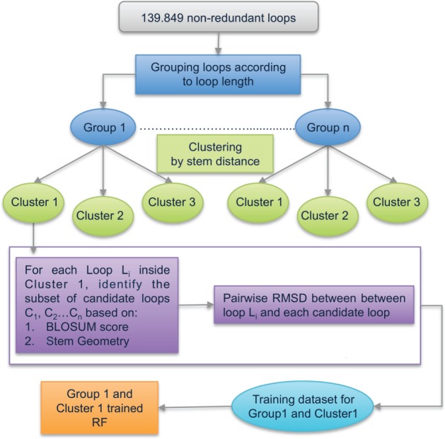
Training procedure workflow

For testing, given a query loop, we first assign it to the appropriate cluster based on its length and stem distance. We next select the corresponding candidate loops and use the appropriate LoopIng model to predict the RMSD distance between the query loop and each of its candidate loops. The candidate loop with the minimum predicted RMSD to the query loop is selected as the best template loop.

Supplementary Figure S1 shows the input features sorted according to their importance in terms of average Mean Decrease Gini values.

2.6 Model building

The modeled structure of the loop is obtained via MODELLER with default parameters (Sali and Blundell, 1993) using the loop with the closest predicted RMSD to the input loop as template. The accuracy of a loop prediction is measured by the backbone RMSD of the predicted and native loops after superimposition of the stems.

3 Results

3.1 Model performance on the CASP10 dataset

Table 1 shows the average performance of the LoopIng method on the CASP10 dataset and the comparison with DisGro and LoopWeaver approaches [using default parameters settings as specified in (Holtby et al., 2013; Tang et al., 2014)], respectively. Overall, LoopIng was able to achieve an average backbone RMSD of 1.29 ± 1.07 Å with statistically significant improvements over DisGro for 8 out of 10 loop length groups. In about half of the cases, LoopIng was able to find a template loop closer than 1 Å with respect to the native loop, achieving a better or significantly better (ΔRMSD ≥ 1 Å) accuracy than DiSGRO in 73 and 44% of the cases, respectively.

Table 1.

Performance comparison between the LoopIng, DisGro (DG) and LoopWeaver (LW) methods on the CASP10 dataset

Loop length (# of cases)	LoopIng (a) (Å)		DG (b) (Å)		LW (c) (Å)		Prediction ≤ 1 Å (d) (%)			LoopIng < DG (e) (%)		LoopIng < LW (f) (%)
	Mean	SD	Mean	SD	Mean	SD	LoopIng	DG	LW	LoopIng  < DG (I)	(DG – LoopIng)  ≥ 1 Å (II)	LoopIng < LW (I)	(LW – LoopIng) ≥ 1 Å (II)
4 (79)	0.74	0.63	1.43*	0.68	0.93	0.64	70	27	47	75	38	52	16
5 (81)	0.85	0.70	1.77*	0.79	1.16*	0.76	62	15	42	76	51	68	23
6(57)	1.06	0.75	2.06*	0.86	1.8*	0.87	58	12	21	83	52	79	38
7(51)	1.6	0.88	2.05*	0.83	2.5*	0.70	29	9	7	61	32	81	39
8(35)	1.88	0.98	2.47*	0.88	2.6*	0.74	24	4	4	72	40	76	40
9(30)	1.7	1.2	2.63*	1.00	3.2*	0.62	45	5	0	60	50	90	45
10(19)	2.4	1.23	3.45*	1.62	3.4*	0.85	22	0	0	76	45	67	56
11(19)	2.38	1.4	3.2	1.9	3.0	1.02	33	0	11	76	56	78	22
12(23)	1.8	1.65	3.55*	1.6	2.69	1.4	46	0	15	77	69	77	46
13(13)	3.1	1.39	3.9	1.8	3.2	1.75	0	0	0	60	0	53	33
Overall (407)	1.29	1.07	2.09	1.44	1.98	1.71	51	14	25	73	44	71	31

Asterisks indicate a statistically significant difference (95% confidence level) with respect to the LoopIng method based on an unpaired t-test. (a, b, c) Mean RMSD and Standard Deviation for LoopIng, DG, and LW respectively. (d) Percentage of cases where LoopIng, DG and LW were able to give a prediction closer than 1 Å with respect to the native loop. (e, f) percentage of cases where LoopIng was more accurate (LoopIng < DG) and significantly better (ΔRMSD ≥ 1 Å) compared to DG and LW respectively.

Compared to LoopWeaver, LoopIng was able to achieve a better or significantly better (ΔRMSD ≥ 1 Å) accuracy in 71 and 31% of the cases, respectively. It is worth noticing that the difference in performance of the two methods increases as the loop length increases.

By and large, the quality of comparative modeling depends on two factors: the availability of reliable template structures and the extent of structural similarity between target and template, which in turn is determined by the extent of the similarity between their sequences (Chothia and Lesk, 1986). In line with this reasoning, we wanted to analyse how much the sequence similarity of the target with the available template loops influences the LoopIng results.

Figure 4 shows the average sequence identity between the loops selected by LoopIng and the target loops and the resulting average RMSD values for the CASP10 benchmark for each loop length group. It can be noticed that the method performance is related to the average local sequence identity between the target loop and the selected template. For example, the average RMSD for loops of length 12 (1.8 ± 1.65 Å) is lower than that obtained for loops of length 11 (2.38 ± 1.4 Å) (Table 1) and this is likely due to the fact that the average target-template sequence identity for loops of length 12 (28%) is higher than that for loops of length 11 (20%) (Fig. 4).

Fig. 4.

Dependence of the model performance expressed in terms of the average RMSD values (x-axis) from the average target-template sequence identity (y-axis) for each loop length group (values inside the bubbles)

Sequence similarity is not the only factor affecting the LoopIng accuracy. Indeed the average backbone RMSD between the LoopIng models and the native conformations also varies with the number of available template loops in the different training set. This impacts more on the performance for long loops (more than 10 residues) since, as it can be appreciated from Figure 1, a much smaller number of training loops are available in this range. This, on the other hand, also implies that the performance of the LoopIng method is likely to improve as the number of available structures increases.

3.2 Model performance on the FREAD benchmark

The benchmark of the FREAD method contains 30 targets for each loop length, (from 4 to 20 residues) and a recent assessment using this benchmark (Choi and Deane, 2010) has shown that template-based methods such as FREAD can achieve better performance compared to the ab-initio loop modeling methods such as MODLOOP, RAPPER and PLOP on this benchmark. A more recent work (Liang et al., 2014) has shown that the ab-initio method LEAP is able to achieve significant improvements over all the other tested methods on the FREAD benchmark.

We therefore tested the performance of LoopIng on the same benchmark and show here the comparison of its results with those of FREAD and LEAP (Table 2). The full comparison between LoopIng and the other methods assessed on the FREAD benchmark is shown in Supplementary Table S2.

Table 2.

Performance of the LoopIng method on the FREAD benchmark

Loop length	Original FREAD		LoopIng		LEAP
	Mean	SD	Mean	SD	Mean	SD
4	1.29*	1.14	0.61	0.55	0.39*	0.23
5	2.19*	2.02	0.68	0.52	0.40*	0.27
6	1.79*	1.37	1.01	0.63	0.49*	0.33
7	2.53*	2.34	1.26	0.9	0.69*	0.38
8	2.88*	2.37	1.47	1.07	0.68*	0.56
9	3.08*	2.60	1.71	1.23	0.93*	0.69
10	4.25*	3.58	1.90	1.34	1.44	0.84
11	4.55*	3.63	1.93	1.48	2.24	1.08
12	3.99*	3.88	2.20	1.70	3.14	2.52
13	5.54*	4.25	2.39	1.85	2.91	2.62
14	6.07*	4.36	2.53	3.03	4.44*	3.70
15	6.41*	5.05	3.05	3.00	4.58	4.16
16	7.50*	6.15	2.82	3.17	4.90*	4.43
17	7.84*	5.27	3.03	3.15	5.66*	5.50
18	5.48	5.64	3.86	3.47	6.53*	6.30
19	7.67*	5.27	3.89	3.51	5.87	4.64
20	7.64*	6.43	3.91	3.49	8.21*	7.82

For each length range the number of tested loops is 30. The columns report the average and standard deviation RMSD values measured between the model and native loop backbone conformations. Asterisks indicate statistically significant differences (95% confidence level) based on an unpaired t-test with respect to the LoopIng model. Underlined values represent the best results between LoopIng and LEAP. The values reported in the FREAD and LEAP columns are taken from Choi and Deane (2010) and Liang et al. (2014), respectively.

The LoopIng results show statistically significant improvements in average accuracy over the FREAD method for all loop lengths (Table 3). For loops of length between 8 and 20 residues, the average improvement is more than 1 Å. It should be mentioned that the reported FREAD data are taken from a relatively old paper (Choi and Deane, 2010) and this can of course affect its performance.

Table 3.

LoopIng performance using native and modeled protein structure

Loop length (# of cases)	Looping_Native (a) Å		Looping_Model (b) Å		ΔRMSD ≤ 0.1 Å (c)	ΔRMSD ≤ 0.5 Å (d)
	Mean	SD	Mean	SD	(%)	(%)
4 (47)	0.58	0.44	0.59	0.67	54	78
5 (33)	0.40	0.39	0.48	0.42	79	92
6(21)	1.23	0.71	1.61	0.57	48	88
7(20)	1.44	1.00	1.77	0.65	45	65
8(9)	1.55	0.99	2.08	0.93	33	33
Overall (130)	0.97	0.80	1.1	0.75	55	73

The performance, in terms of backbone RMSD with respect to the native loop conformation, using (a) the native structure for the remaining portion of the protein (LoopIng_Native) and (b) the best CASP10 predicted model (LoopIng_Model). (c) Percentage of cases where the RMSD difference between LoopIng_Native and LoopIng_Model is ≤ 0.1 Å. (d) Percentage of cases where the RMSD difference between LoopIng_Native and LoopIng_Model ≤ is 0.5 Å.

Furthermore, Choi and Deane (2010) showed that the performance of FREAD can be enhanced by setting a much stricter similarity threshold. However, this choice results in a much lower coverage especially for loops longer than eight residues (coverage < 60%). Compared to this modified version of FREAD, LoopIng still shows an improvement for short and medium length loops while FREAD reaches higher accuracy for longer loops, although the coverage is lower than 50% in these cases (Supplementary Table S3).

The accuracy of LEAP and LoopIng on the FREAD benchmark is very similar. Notably, LEAP is more accurate for short loops (from 4 to 9 residues) while LoopIng seems to work better (ΔRMSD ≥ 1 Å) for longer loops (Table 2). It is worth noticing that the LoopIng method is rather fast, it takes on average 1 min/loop (CPU speed: 2.5 GHz and RAM: 2 GB) to be compared with an average running time of 10 h/loop for the LEAP method.

It would have been interesting to compare LoopIng and LEAP also on the CASP10 benchmark, but this turned out to be unfeasible since the LEAP results are only available for a limited subset of the targets (namely 21), the definition of the loops seems to be different and only the median accuracy is provided by the authors (Liang et al., 2014).

3.3 Model performance on non-native protein structures

Both LoopIng and other template-based methods (i.e. FREAD, LoopWeaver) use the stem distance as a filtering step to select the top template loop(s) from a database of known structures. However, in a more realistic setting, the native structure of the remaining part of the protein is usually unknown, and the loop is built on the basis of a modeled structure. In these cases, the stem structure is very likely to be affected by errors. We tested to which extent this affects the accuracy of LoopIng.

To do so, we downloaded the best model submitted to CASP10 [according to the GDT-TS measure (Huang et al., 2014)] for each target protein. If there was more than one, we selected the model with the lowest Cα RMSD. Only modeled structures with GDT-TS score ≥ 50 are considered for this test set to ensure that the models were based on a detectable and appropriate template (Kinch et al., 2011). This resulted in a dataset of 130 non-redundant loops (Table 3).

Table 3 illustrates the difference in performance, in terms of backbone RMSD between the model and native loop, when the native structure or the model is used. The performance is very similar as the mean RMSD values are 0.97 ± 0.80 and 1.1 ± 0.75 Å, respectively. In 55% of the cases the two predictions (using the native structure and the modeled one) selected almost identical loop template (RMSD ≤ 0.1 Å) with respect to the native loop conformation.

The difference in performance between using the native (LoopIng_Native) and modeled (LoopIng_Modeled) structure for the rest of the protein is shown in Figure 5 as a function of the stem distance error. The LoopIng model shows similar performance (≤ 1 Å) when using the native and the modeled structure when the stem distance error is lower than 2.0 Å.

Fig. 5.

Model performance using native and modeled protein structures from CASP10 dataset. The stem distance error (x-axis) is calculated as the difference in stem distance between the modeled and native stem structures. The RMSD error (y-axis) is calculated as the difference in backbone RMSD between LoopIng_Native and LoopIng_Model

4 Conclusions

We describe here a new template-based method for predicting the structure of protein loops, a complex, yet critical, problem that is considered one of the bottlenecks for accurately predicting protein structures.

The method was able to achieve significant enhancements over other available methods both template-based (i.e. LoopWeaver and FREAD) and ab-initio (i.e. DiSGRO) with an average improvement of the backbone RMSD close to 1 Å. It was also able to achieve comparable results to those of the LEAP method with a running time orders of magnitude faster.

The quality of the predictions is not dependent upon the fine details of the stem geometry, indicating that the method is robust to errors that unavoidably affect these regions when they are modeled rather than taken from the native structure.

Our analysis also suggests that combined methods (ab-initio and template-based) might be worth investigating. Short loops are efficiently modeled using ab-initio methods (i.e. LEAP) due to the small number of degrees of freedom, which permits an adequate exploration of the conformational space, while long loops are more effectively predicted using template-based methods (i.e. LoopIng).

We believe that the method can be a useful addition to the presently available protein structure prediction tools and could be effectively and easily integrated in comparative modeling pipelines.

Funding

KAUST Award No. KUK-I1-012-43 made by King Abdullah University of Science and Technology (KAUST) and PRIN No. 20108XYHJS.

Conflict of Interest: none declared.

References

- Browne W.J., et al. (1969) A possible three-dimensional structure of bovine alpha-lactalbumin based on that of hen's egg-white lysozyme. J. Mol. Biol., 42, 65–86. [DOI] [PubMed] [Google Scholar]
- Bruccoleri R.E., Karplus M. (1990) Conformational sampling using high-temperature molecular dynamics. Biopolymers, 29, 1847–1862. [DOI] [PubMed] [Google Scholar]
- Canutescu A.A., Dunbrack R.L., Jr. (2003) Cyclic coordinate descent: a robotics algorithm for protein loop closure. Protein Sci. Publ. Protein Soc., 12, 963–972. [DOI] [PMC free article] [PubMed] [Google Scholar]
- Choi Y., Deane C.M. (2010) FREAD revisited: accurate loop structure prediction using a database search algorithm. Proteins, 78, 1431–1440. [DOI] [PubMed] [Google Scholar]
- Chothia C., Lesk A.M. (1986) The relation between the divergence of sequence and structure in proteins. EMBO J., 5, 823–826. [DOI] [PMC free article] [PubMed] [Google Scholar]
- Deane C.M., Blundell T.L. (2000) A novel exhaustive search algorithm for predicting the conformation of polypeptide segments in proteins. Proteins, 40, 135–144. [PubMed] [Google Scholar]
- Deane C.M., Blundell T.L. (2001) CODA: a combined algorithm for predicting the structurally variable regions of protein models, Protein Sci. Publ. Protein Soc., 10, 599–612. [DOI] [PMC free article] [PubMed] [Google Scholar]
- de Bakker P.I.W., et al. (2003) Ab initio construction of polypeptide fragments: accuracy of loop decoy discrimination by an all-atom statistical potential and the AMBER force field with the generalized born solvation model. Proteins, 51, 21–40. [DOI] [PubMed] [Google Scholar]
- Eyal E., et al. (2005) The limit of accuracy of protein modeling: influence of crystal packing on protein structure. J. Mol. Biol., 351, 431–432 [DOI] [PubMed] [Google Scholar]
- Felts A.K., et al. (2008) Prediction of protein loop conformations using the AGBNP implicit solvent model and torsion angle sampling. J. Chem. Theory Comput., 4, 855–868. [DOI] [PMC free article] [PubMed] [Google Scholar]
- Fernandez-Fuentes N., Fiser A. (2006) Saturating representation of loop conformational fragments in structure databanks. BMC Struct. Biol., 6, 15. [DOI] [PMC free article] [PubMed] [Google Scholar]
- Fetrow J.S., et al. (1998) Functional analysis of the Escherichia coli genome using the sequence-to-structure-to-function paradigm: identification of proteins exhibiting the glutaredoxin/thioredoxin disulfide oxidoreductase activity. J. Mol. Biol., 282, 703–711. [DOI] [PubMed] [Google Scholar]
- Finkelstein A.V., Reva B.A. (1992) Search for the stable state of a short chain in a molecular field. Protein Eng., 5, 617–624. [DOI] [PubMed] [Google Scholar]
- Fiser A., et al. (2000) Modeling of loops in protein structures. Protein Sci. Publ. Protein Soc., 9, 1753–1773. [DOI] [PMC free article] [PubMed] [Google Scholar]
- Henikoff S., Henikoff J.G. (1992) Amino acid substitution matrices from protein blocks. Proc. Natl Acad. Sci. USA, 89, 10915–10919. [DOI] [PMC free article] [PubMed] [Google Scholar]
- Higo J., et al. (1992) Development of an extended simulated annealing method: application to the modeling of complementary determining regions of immunoglobulins. Biopolymers, 32, 33–43. [DOI] [PubMed] [Google Scholar]
- Holtby D., et al. (2013) LoopWeaver: loop modeling by the weighted scaling of verified proteins. J. Comput. Biol. J. Comput. Mol. Cell Biol., 20, 212–223. [DOI] [PMC free article] [PubMed] [Google Scholar]
- Huang Y., et al. (2010) CD-HIT Suite: a web server for clustering and comparing biological sequences. Bioinformatics, 26, 680–682. [DOI] [PMC free article] [PubMed] [Google Scholar]
- Huang Y.J., et al. (2014) Assessment of template-based protein structure predictions in CASP10. Proteins, 82, 43–56. [DOI] [PMC free article] [PubMed] [Google Scholar]
- Jacobson M.P., et al. (2004) A hierarchical approach to all-atom protein loop prediction. Proteins, 55, 351–367. [DOI] [PubMed] [Google Scholar]
- Jones S., Thornton J.M. (1997) Prediction of protein-protein interaction sites using patch analysis. J. Mol. Biol., 272, 133–143. [DOI] [PubMed] [Google Scholar]
- Kabsch W., Sander C. (1983) Dictionary of protein secondary structure: pattern recognition of hydrogen-bonded and geometrical features. Biopolymers, 22, 2577–2637. [DOI] [PubMed] [Google Scholar]
- Kick E.K., et al. (1997) Structure-based design and combinatorial chemistry yield low nanomolar inhibitors of cathepsin D. Chem. Biol., 4, 297–307. [DOI] [PubMed] [Google Scholar]
- Kinch L.N., et al. (2011) CASP9 target classification. Proteins, 79, 21–36. [DOI] [PMC free article] [PubMed] [Google Scholar]
- Kryshtafovych A., et al. (2014) Challenging the state-of-the-art in protein structure prediction: highlights of experimental target structures for the 10(th) Critical Assessment of Techniques for Protein Structure Prediction Experiment CASP10. Proteins, 82, 26–42. [DOI] [PMC free article] [PubMed] [Google Scholar]
- Lessel U., Schomburg D. (1999) Importance of anchor group positioning in protein loop prediction. Proteins, 37, 56–64. [PubMed] [Google Scholar]
- Liang S., et al. (2014) LEAP: highly accurate prediction of protein loop conformations by integrating coarse-grained sampling and optimized energy scores with all-atom refinement of backbone and side chains. J. Comput. Chem., 35, 335–341. [DOI] [PMC free article] [PubMed] [Google Scholar]
- Marti-Renom M.A., et al. (1998) Statistical analysis of the loop-geometry on a non-redundant database of proteins. J. Mol. Mod., 4, 347–354. [Google Scholar]
- Marti-Renom M.A., et al. (2000) Comparative protein structure modeling of genes and genomes. Annu. Rev. Biophys. Biomol. Struct., 29, 291–325. [DOI] [PubMed] [Google Scholar]
- Mattos C., et al. (1994) Analysis of two-residue turns in proteins. J. Mol. Biol., 238, 733–747. [DOI] [PubMed] [Google Scholar]
- Messih M.A., et al. (2014) Improving the accuracy of the structure prediction of the third hypervariable loop of the heavy chains of antibodies. Bioinformatics, 30, 2733–2740. [DOI] [PMC free article] [PubMed] [Google Scholar]
- Moult J., et al. (2014) Critical assessment of methods of protein structure prediction (CASP)—round x. Proteins, 82, 1–6. [DOI] [PMC free article] [PubMed] [Google Scholar]
- Oliva B., et al. (1997) An automated classification of the structure of protein loops. J. Mol. Biol., 266, 814–830. [DOI] [PubMed] [Google Scholar]
- Rapp C.S., Friesner R.A. (1999) Prediction of loop geometries using a generalized born model of solvation effects. Proteins, 35, 173–183. [PubMed] [Google Scholar]
- Russell R.B., et al. (1998) Supersites within superfolds. Binding site similarity in the absence of homology. J. Mol. Biol., 282, 903–918. [DOI] [PubMed] [Google Scholar]
- Spassov V.Z., et al. (2008) LOOPER: a molecular mechanics-based algorithm for protein loop prediction. Protein Eng. Des. Selection PEDS, 21, 91–100. [DOI] [PubMed] [Google Scholar]
- Schwede T. (2013) Protein modeling: what happened to the “protein structure gap”? Structure, 21, 1531–1540. [DOI] [PMC free article] [PubMed] [Google Scholar]
- Tang K., et al. (2014) Fast protein loop sampling and structure prediction using distance-guided sequential chain-growth Monte Carlo method. PLoS Comput. Biol., 10, e1003539. [DOI] [PMC free article] [PubMed] [Google Scholar]
- Venclovas C., et al. (2003) Assessment of progress over the CASP experiments. Proteins, 53, 334–339. [DOI] [PubMed] [Google Scholar]
- Wang G., Dunbrack R.L., Jr. (2003) PISCES: a protein sequence culling server. Bioinformatics, 19, 1589–1591. [DOI] [PubMed] [Google Scholar]
- Xiang Z., et al. (2002) Evaluating conformational free energies: the colony energy and its application to the problem of loop prediction. Proc. Natl Acad. Sci. USA, 99, 7432–7437. [DOI] [PMC free article] [PubMed] [Google Scholar]
- Zhou H., Zhou Y. (2002) Distance-scaled, finite ideal-gas reference state improves structure-derived potentials of mean force for structure selection and stability prediction. Protein Sci., 11, 2714–2726. [DOI] [PMC free article] [PubMed] [Google Scholar]
Associated Data
This section collects any data citations, data availability statements, or supplementary materials included in this article.