

Abstract
The density of liquid toluene has been measured over the temperature range −60 °C to 200 °C with pressures up to 35 MPa. A two-sinker hydrostatic-balance densimeter utilizing a magnetic suspension coupling provided an absolute determination of the density with low uncertainties. These data are the basis of NIST Standard Reference Material® 211d for liquid density over the temperature range −50 °C to 150 °C and pressure range 0.1 MPa to 30 MPa. A thorough uncertainty analysis is presented; this includes effects resulting from the experimental density determination, possible degradation of the sample due to time and exposure to high temperatures, dissolved air, uncertainties in the empirical density model, and the sample-to-sample variations in the SRM vials. Also considered is the effect of uncertainty in the temperature and pressure measurements. This SRM is intended for the calibration of industrial densimeters.
Keywords: calibration, density, standard reference material, toluene, uncertainty
1. Introduction
The property of fluid density is a vital parameter in a multitude of industrial processes. These include the control of chemical processes and the metering of fuels and other commodity chemicals. Often, the process stream is sampled through an industrial densimeter for continuous, real-time determination of the density. Such densimeters are not absolute instruments—they must be regularly calibrated at the conditions of use with fluids of known density.
The work presented here utilizes an absolute fluid densimeter to establish the density of toluene as a function of temperature and pressure for use as a calibration standard. The measured density data are presented, but of more relevance for calibration purposes, the density data are also represented in terms of an empirical function relating temperature, pressure, and density.
Toluene has a number of advantages as a density standard: it is a stable chemical of relatively low toxicity; its density of 865 kg/m3 at ambient conditions is well matched to many applications; its freezing point of −95 °C and boiling point of 111 °C cover the range of many industrial processes. Toluene has a low surface tension compared to that of water, and it is relatively inexpensive. The National Institute of Standards and Technology (NIST) has sold a density Standard Reference Material (SRM®) based on toluene for many years, but the previous SRM was certified only at ambient conditions: 15 °C to 25 °C and normal atmospheric pressure.
This SRM certifies the density of a particular batch of toluene. This approach is preferred for high-accuracy calibrations over the alternative approach of measuring the density of “very pure” toluene for at least two reasons. First, a batch certification is directly traceable to NIST, and this is often a requirement for high-level calibration laboratories. Second, toluene in very high purities is difficult to obtain. High-quality commercial toluene (e.g., reagent grade or HPLC grade) is usually intended for use as a chemical precursor or as a solvent in various chemical analyses; it is certified to be free of contaminants (such as sulfur compounds) that would affect the analysis, but other impurities, such as closely related organic compounds, are often present. The use of “pure” toluene would greatly complicate the traceability of density and shift the problem to one of determining purity and/or the effects of impurities on the density.
This work describes the development of an extended-range SRM (designated as SRM 211d) for fluid density over wide ranges of temperature and pressure. First, the experimental principle, apparatus, and procedures are described. A description of the calibration procedures establishes traceability to SI quantities. The most significant uncertainties in the experimental determination of the fluid density are shown to arise from uncertainties in the sinker volumes, and the calibration of the sinker volumes is described in detail. Sections 4 and 5 present the results and a thorough analysis of the uncertainties.
2. Experimental Determination of Density
2.1 Experimental Principle
The two-sinker densimeter used in this work is described in detail by McLinden and Lösch-Will [1], and this general type of instrument is described by Wagner and Kleinrahm [2]. In the present densimeter two sinkers of nearly the same mass, surface area, and surface material, but very different volumes, are weighed separately with a high-precision balance while immersed in a fluid of unknown density. The fluid density ρ is given by
| (1) |
where m and V are the sinker mass and volume, W is the balance reading, and the subscripts refer to the two sinkers. The main advantage of the two-sinker method is that adsorption onto the surface of the sinkers, systematic errors in the weighing, and other effects that reduce the accuracy of most buoyancy techniques cancel.
A magnetic suspension coupling transmits the gravity and buoyancy forces on the sinkers to the balance, thus isolating the fluid sample (which may be at high pressure and/or extremes of temperature) from the balance. The central elements of the coupling are two magnets, one on each side of a nonmagnetic pressure-separating wall. The top magnet, which is an electromagnet with a ferrite core, is hung from the balance. The bottom (permanent) magnet is held in stable suspension with respect to the top magnet by means of a feedback control circuit making fine adjustments in the electromagnet current. The permanent magnet is linked with a lifting device to pick up a sinker for weighing. A mass comparator with a resolution of 1 μg and a capacity of 111 g is used for the weighings. Each sinker has a mass of 60 g; they are fabricated of tantalum and titanium and are both gold plated.
Equation (1) must be corrected for magnetic effects; this is described by McLinden et al. [3]. In addition to the sinkers, two calibration masses are also weighed. Figure 1 shows a schematic of the density measuring cell and the four weighings. The weighings yield a set of four equations that are solved to yield, first, a balance calibration factor α and a parameter β related to the balance tare (i.e., those elements of the system that are always weighed):
| (2) |
| (3) |
where the subscripts cal and tare refer to the calibration weights; ρair is the density of the air (or purge gas) surrounding the balance and is calculated from the ambient temperature, pressure, and humidity measured in the balance chamber. In all the measurements reported here, the balance chamber was continuously purged with nitrogen. The “coupling factor” ϕ, which is the efficiency of the force transmission of the magnetic suspension coupling, is given by
| (4) |
Fig. 1.

Schematic of the two-sinker densimeter showing the four weighings; (a) weighing of the tantalum sinker, (b) weighing of the titanium sinker, (c) weighing of the balance calibration weight, and (d) weighing of the balance tare weight; in (c) and (d) both sinkers are on their rests. Balance displays are typical for a fluid density of 941 kg/m3. Figure is not to scale.
Finally, the fluid density ρfluid is given by
| (5) |
where ρ0 is the indicated density when measuring in vacuum. In other words ρ0 is an “apparatus zero,” which compensates for any changes in alignment or sinker masses. (The sinker masses were observed to change on the order of a few μg due to surface contamination and physical wear where they were picked up. Any shift in the alignment of the magnetic suspension coupling will result in a slight change in the apparent sinker masses.) The key point of the analysis by McLinden et al. [3] is that the density given by Eq. (5) compensates for the magnetic effects of both the apparatus and fluid being measured. With this apparatus, the coupling factor is nearly unity; for the present results it varied from 1.000 020 for vacuum to 0.999 975 for toluene at the highest density measured.
2.2 Apparatus Description
In addition to the sinkers, suspension coupling, and balance that make up the density measuring system, the apparatus includes a thermostat, pressure instrumentation, and a sample handling system. A schematic diagram of the densimeter is shown as Fig. 2.
Fig. 2.
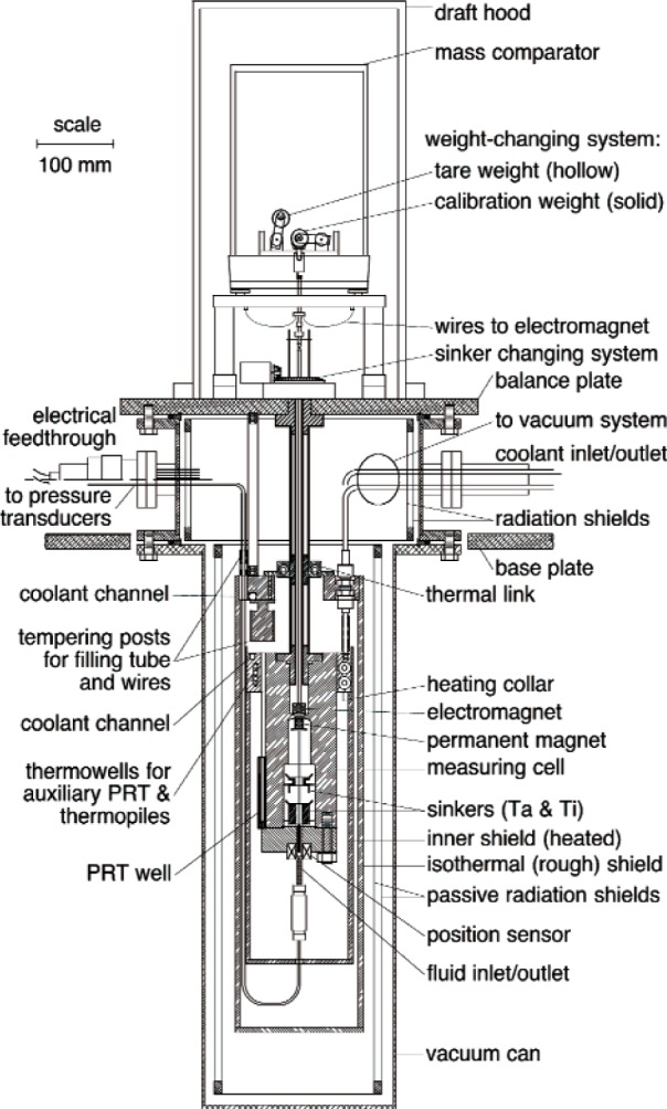
Detailed schematic of the density system and thermostat.
The temperature is measured with a standard-reference-quality platinum resistance thermometer (SPRT) and resistance bridge referenced to a thermostatted standard resistor. The signal from the SPRT is used directly in a digital control circuit to maintain the cell temperature constant within ± 0.001 K. The pressures are measured with state-of-the-art transducers combined with careful calibration. The transducers (as well as the pressure manifold) are thermostatted to minimize the effects of variations in laboratory temperature.
The thermostat serves to isolate the measuring cell from ambient. It is a vacuum-insulated, cryostat-type design. The measuring cell is surrounded by an isothermal shield, which thermally isolates it from variations in ambient temperature; this shield was maintained at a constant (± 0.01 K) temperature 1 K below the cell temperature. Electric heaters compensate for the small heat flow from the cell to the shield and allow millikelvin-level control of the cell temperature. Operation at sub-ambient temperatures is effected by circulating ethanol from a chiller through channels in the shield.
2.3 Experimental Material
The material used is identical to the previous SRM, which is described as “a high purity liquid toluene … obtained from a commercial source.” [4] The SRM is provided in 5 mL flame-sealed glass ampoules. At the same time the 5 mL ampoules were prepared, several large 1.5 L flame-sealed ampoules were also prepared containing the same toluene. We worked with material from one of the 1.5 L ampoules, except for some of the chemical analysis, which used the 5 mL ampoules. We transferred the toluene from the 1.5 L ampoule to a 2.5 L stainless-steel sample cylinder for convenience in sample handling.
The sample was degassed by freezing the stainless-steel cylinder in liquid nitrogen, evacuating the vapor space, and thawing. The freeze/pump/thaw process was repeated a total of three times. The residual pressure over the frozen sample on the final cycle was 0.0002 Pa. The SRM as supplied by NIST contains some amount of dissolved air. The sample was degassed to obtain a well characterized state for the measurements. Also, we were concerned that dissolved air could react with the toluene at the elevated temperatures measured in this work. We felt that the uncertainties introduced by “purifying” the SRM material in this way would be offset by a reduction in possible effects resulting from reaction of the toluene with air. This point is discussed further in Sec. 4.3.
A chemical analysis by gas chromatography-mass spectrometry revealed the presence of trace levels of dimethyl benzenes and ethyl benzene; these are heavier impurities that would be expected to be present in toluene. A quantitative analysis by gas chromatography with a flame ionization detector yielded an overall purity of 99.92 % toluene with a standard uncertainty of 0.01 %. The sample was collected following the density measurements and reanalyzed; no significant differences were detected.
To quantify the effect of dissolved air on the density, additional measurements were made on a sample that was saturated with air at a temperature of 20 °C and pressure of 0.10 MPa. A quantity of the degassed toluene was transferred to an evacuated 500 mL stainless steel sample cylinder. Dry air was admitted to the cylinder to a pressure of 0.10 MPa; additional air was admitted periodically over the course of 24 hours to maintain the pressure at 0.10 MPa. The cylinder was periodically mixed to promote equilibrium. The air used was commercial “breathing air” with a moisture specification of 3 ppm. (Breathing air is air of normal atmospheric composition that has been dried.)
2.4 Experimental Procedures
Each density determination involved weighings in the order: tantalum (Ta) sinker, titanium (Ti) sinker, balance calibration weight, balance tare weight, balance tare weight (again), balance calibration weight, Ti sinker, and Ta sinker, for a total of eight weighings—two for each object. For each weighing, the balance was read five times over the course of ten seconds. For each object, the ten balance readings were averaged for use in Eqs. (2 to 5). Between each of the object weighings, and also before the first weighing and following the final weighing, the temperature and pressure were recorded, for a total of nine readings of t and p; these were also averaged. A complete density determination required 12 min. The weighing design was symmetrical with respect to time, and this tended to cancel the effects of any drift in the temperature or pressure.
The sample was loaded at a low temperature and pressure. Higher pressures were generated by heating the liquid-filled cell; this avoided the need for any type of compressor, which could have been a source of contamination, such as residual material from a previous test fluid. Starting at the lowest temperature and pressure for a given filling, measurements were made at increasing temperatures (and nearly constant density) until the maximum desired pressure was reached. The sample was then vented to a lower pressure along an isotherm.
The densimeter control program monitored the system temperatures and pressures once every 60 seconds. A running average and standard deviation of the temperatures and pressures were computed for the preceding eight readings. When these were within preset tolerances of the set-point conditions, a weighing sequence was triggered. Once the specified number of replicate density determinations were made at a given (t,p) state point, the control program then moved to the next temperature or automatically vented the sample to the next pressure on an isotherm.
Between each filling, and also before the first filling and following the last filling, the system was evacuated and the density recorded multiple times. The indicated density was used to determine the apparatus zero ρ0. The value of ρ0 used in Eq. (5) is the time-weighted average of ρ0 values measured before and after a given density determination.
3. Calibrations
3.1 Temperature and Pressure
The main platinum resistance thermometer (SPRT) used to measure the temperature of the fluid was calibrated on ITS–90 from 83 K to 505 K by use of fixed point cells (argon triple point, mercury triple point, water triple point, indium freezing point and tin freezing point). This was done as a system calibration, meaning that the SPRT was removed from its thermo-well in the measuring cell and inserted into the fixed point cell using the same lead wires, standard resistor, and resistance bridge that were used in the density measurements. The manufacturers of the fixed points have certified traceability to NIST and provide a temperature uncertainty of 1 mK or less. The fixed points and our calibration procedures were verified by checking each of the fixed point systems against a NIST-calibrated SPRT.
A full calibration of the main SPRT was carried out two months prior to the beginning of the toluene measurements. The resistance at the triple point of water was checked 16 months later; the resistance had changed by the equivalent of 0.5 mK. The standard (k = 1) uncertainty in the temperature, including uncertainty in the fixed point cells, drift in the SPRT, and temperature gradients between the SPRT and the actual fluid sample, is estimated to be 2 mK.
The pressure transducer was calibrated with a hybrid gas-oil piston gage system at pressures up to 40 MPa. Again, this calibration was done in-situ by connecting the piston gage to the sample port of the filling manifold. Based on the uncertainty for the piston gage, the repeatability observed for these transducers, and the uncertainties associated with the hydrostatic head correction, we estimate the standard uncertainty in pressure to be [(0.000026 · p)2 + (2.0 kPa)2]0.5, where the first term arises from uncertainties in the calibration, and the second term is a conservative estimate of the uncertainties arising from the head correction and the drift in the pressure transducer between calibrations.
3.2 Balance Calibration
An automated calibration of the mass comparator (i.e., the α in Eq. (2)) is an integral part of each density determination; it was achieved by a mechanism that lowers tare and calibration weights onto a modified balance pan. (The tare weight is required because the balance has a limited weighing range; without the tare weight, the balance would be “under-range.”) The weights were cylindrical in shape and fabricated of stainless steel (calibration weight) and hollow stainless steel (tare weight) with a mass difference of 15.2 g. The masses of these weights were determined by an SXXS-type comparison to standard masses [5]. The correction for air buoyancy on the standard mass was calculated by use of the BIPM air density equation [6] with ambient conditions measured with an electronic barometer and a temperature and humidity transmitter with the sensor located next to the balance.
The two weights were nearly identical in volume and surface area. The volumes of the calibration weights were determined by a simple hydrostatic determination using water as the density reference. Each volume was determined to be 7.4788 cm3. This provided a balance calibration that is very nearly independent of the density of the air or nitrogen purge gas surrounding the balance.
3.3 Sinker Volumes at 20 °C
Uncertainty in the sinker volumes was the major component of the overall fluid density uncertainty (as discussed in Sec. 5), and considerable effort was expended in determining these volumes accurately. The sinker volumes were determined using the hydrostatic comparator technique described by Bowman et al. [7,8]. This method differs from the traditional hydrostatic technique in that the known density is that of a solid object rather than that of a reference fluid, such as water. The standard and unknown objects are suspended in a fluid, but the fluid serves only to transfer the density knowledge of the standard to that of the unknown. The density of the fluid itself need not be known—it needs only to be constant during the period necessary to complete the measurement.
3.3.1 Hydrostatic Apparatus
A separate apparatus has been developed at NIST to carry out the sinker volume determinations. It is modeled closely after the apparatus of Bowman et al. [7]. A thermostatted fluid bath contains a “stage” that allows the submerged objects to be placed one at a time onto a weighing “pan” that is suspended from the weighing hook of an analytical balance. The apparatus is shown in Fig. 3.
Fig. 3.
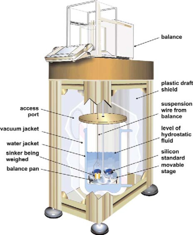
Cut-away view of the hydrostatic apparatus used to determine sinker volumes.
The fluid bath is a custom-built triple-walled beaker of borosilicate glass. The inner volume (approximately 170 mm inside diameter by 295 mm high) contains the hydrostatic fluid. It is surrounded by a water jacket connected to a circulating bath. The outermost jacket is evacuated for thermal insulation. A brass cover plate serves to minimize evaporation and temperature gradients. The bath is contained within a sturdy aluminum frame with plastic side panels to control drafts. The frame is topped by a 40 kg limestone block on which the balance sits.
The bath fluid is a high-density fluoroether (2-trifluoromethyl-3-ethoxydodecafluorohexane). This fluid has several advantages over water. Its high density of approximately 1631 kg/m3 increases the buoyancy force on the submerged objects and thus the sensitivity of the volume determination. Its lower surface tension (16 N/m compared to 73 N/m for water) decreases the forces on the suspension wire. This and the much higher gas solubility compared to that of water greatly reduce the problems associated with small air bubbles clinging to the objects.
The temperature of the fluid bath was measured with a standard-reference-quality SPRT in a thermowell located in close proximity to the weighing pan. The SPRT was calibrated on ITS–90 at the triple point of water (0.01 °C) and the melting point of gallium (29.7646 °C). The circulating bath was started at least 16 hours prior to the weighings to allow temperature equilibrium to be achieved. During the weighings, the standard deviation of the bath temperature was 1.7 mK, with a maximum deviation of 6 mK from the average value of 293.135 K.
The stage is a simple “turntable” that holds the objects to be weighed. It was manually lifted and rotated (using a central axle extending above the bath cover plate) to place the objects on the weighing pan. The weighing pan was suspended from the balance with a stainless steel wire 0.08 mm in diameter. The balance had a capacity of 205 g, resolution of 10 μg, and linearity of 30 μg. The balance was calibrated immediately before each determination with its built-in calibration weights and automatic calibration sequence. The balance was then checked with a 100 g standard mass (class E2; certified mass 99.999 94 ± 0.000 05 g). The balance reading was consistently low by an average of 0.14 mg, and an adjustment of 1.4 ppm was applied to all subsequent balance readings to compensate for this difference.
The standards are made of hyperpure, float-zone, single-crystal silicon. They are in the shape of right circular cylinders (49.8 mm diameter by 22.1 mm high) with a nominal mass of 100 g. Their densities were determined and certified by the NIST Mass Group [9] with an expanded (k = 2) uncertainty of 0.000 032 g/cm3, which is equal to 0.0014 % of their density of 2.329 095 g/cm3. This determination was carried out using techniques very similar to those described here. The density standards used by the NIST Mass Group were silicon crystals that are the U.S. national solid-density standards. In fact, they are the artifacts described by Bowman et al. [7], which are directly traceable to densities determined by dimensional measurements of near-perfect spheres by interferometry and mass measurements commencing with the U.S. national mass standards. Silicon is an ideal density standard because single-crystal material of very high purity is readily available at moderate cost. Its coefficient of thermal expansion and, thus, variation in density as a function of temperature, are known very well [10].
3.3.2 Experimental Design
The hydrostatic apparatus accommodates four objects—two standards and two unknowns. This allows the simultaneous determination of the volumes of the tantalum and titanium sinkers and also provides the redundancy that permits a statistical analysis of the measurements. The experiment involves a series of A-B-A type weighings to yield ratios of the volumes of A and B. Bowman et al. [7] described a set of 15 weighings needed to determine six volume ratios. Here, the design was modified slightly to 16 weighings:
where “A” is standard #1, “B” is the tantalum sinker, “C” is standard #2, and “D” is the titanium sinker. This design yields the ratios AB, AC, AD, DA, DB, DC, CD, CB and BC, or three more ratios than in the Bowman sequence, for only one additional weighing.
Each “weighing” in the experimental design consisted of the following steps:
Raise and rotate the stage to place the desired object into position above the weighing pan (this is defined as time 0:00).
Record the bath temperature and the balance reading for the empty weighing pan at time 8:00. (Rotation of the stage causes turbulence in the bath, and so several minutes were needed for this to subside.)
Lower the stage to place the object onto the weighing pan shortly after step 2 (approximately 8:30 to 9:00).
Record the bath temperature and the balance reading for the loaded weighing pan at time 16:00.
This sequence was repeated 15 more times (plus an additional weighing of the empty pan at the end) for a total elapsed time of 264 min. The thermometer and balance readings were recorded by computer within a few milliseconds of the specified times. This strict adherence to timing and the A-B-A design compensated for any linear drift in the balance zero and/or drift in the fluid density over the course of the experiment. The time between weighings was more than adequate to allow turbulence to subside (steady weighings were typically observed within three minutes of moving the stage). Also, the object was in the proximity of the SPRT for nearly 15 min before it was weighed, allowing time for temperature equilibration with the fluid in the vicinity of the SPRT. At the end of the complete weighing sequence the balance was tared (but not recalibrated) and again checked with the 100 g class E2 mass; the drift was less than 0.08 mg.
The masses of the sinkers and standards were determined at least twice on different days and the average value used in the analysis. A conventional mass determination in air was carried out using the balance. The correction for air buoyancy was calculated with the BIPM air density equation [6] with ambient conditions measured with an electronic barometer and a temperature and humidity transducer with the sensor located next to the balance.
Each balance weighing W is a summation of mass and buoyancy terms. For the empty pan
| (6) |
where m is mass, V is volume and ρ is density. For the pan loaded with object “B”
| (7) |
The (1 − ρair/ρweights) terms correct for air buoyancy— the balance was calibrated in air with stainless steel calibration masses with density ρweights, but the submerged objects are not subject to air buoyancy. The air density in Eqs. (6) and (7) is that at the time of the balance calibration.
The average of the pan weighings immediately preceding and following each object weighing were subtracted from Eq. (7) to yield
| (8) |
(Equations (6) to (8) are properly written in terms of force, not mass, since the balance used is a force transducer. But the acceleration of gravity cancels, and, by convention, the m × g force measured by the balance is recorded in terms of mass.)
Combining Eq. (8) with the average of two similar equations for the weighings of a second object immediately preceding and following the weighing of object B (i.e., the weighings of a A-B-A sequence) cancels the fluid density to yield the volume ratio:
| (9) |
The measured volume ratios were determined at a temperature that differed slightly from the desired reference temperature of 20 °C. A small (maximum 0.26 ppm) correction was applied using literature values of the thermal expansion coefficient (Swenson [10] for silicon and Touloukian et al. [11] for tantalum and titanium) to adjust the volume ratios to the reference temperature.
3.3.3 Results for Sinker Volumes
The volume ratios and resulting sinker volumes are given in Table 1. The experimental design provides a number of consistency checks. The repeat determinations of the volumes were very consistent, with a standard deviation of 0.000 003 cm3 for the tantalum sinker and 0.000 023 cm3 for the titanium sinker. Knowledge of the fluid density is not required, but the fluid density can be calculated from the results. (In fact, the apparatus serves as a highly sensitive single-sinker densimeter.) The fluid density was observed to have a nearly constant linear drift of 0.55 × 10⁻⁶ ρ/hr. This could be due to a drift in the balance calibration and/or absorption of air and water into the fluid, but in either case the effect was negligible over the 48 min required to complete an A-B-A weighing sequence.
Table 1.
Volume ratios and volumes determined by hydrostatic weighing
| Object | Ratio | Measured Volume Ratio | Ratio Adjusted to 20 °C | Mass (g) |
Volume (cm3) |
|---|---|---|---|---|---|
| tantalum sinker | AB | 11.746 127 | 11.746 129 | 3.610 246 | |
| CB | 11.774 715 | 11.774 718 | 3.610 248 | ||
| BC | 0.084 928 | 0.084 928 | 3.610 242 | ||
| average | 60.177 96 | 3.610 245 | |||
| σ = 0.000 003 | |||||
| titanium sinker | AD | 3.177 097 | 3.177 098 | 13.347 530 | |
| DA | 0.314 753 | 0.314 753 | 13.347 530 | ||
| DC | 0.313 989 | 0.313 989 | 13.347 572 | ||
| CD | 3.184 823 | 3.184 824 | 13.347 566 | ||
| average | 60.163 41 | 13.347 549 | |||
| σ = 0.000 023 |
The experimental design also yields the volume ratios of the two standards and of the two sinkers; these allow a further check of consistency. The measured volume ratio of the silicon standards (ratio AC) can be compared to the value calculated with the known values of mass and density. The directly measured ratio of the sinker volumes (ratio DB) can be compared to the value obtained from the volumes calculated from the other ratios. These are compared in Table 2 and are seen to be well within the expected uncertainties discussed below.
Table 2.
Volume ratios determined by hydrostatic weighing compared to calculated values
| Ratio | Measured Value | Calculated Value | Difference |
|---|---|---|---|
| AC | 0.997 576 | 0.997 571 | 0.000 005 |
| DB | 3.697 088 | 3.697 131 | −0.000 043 |
4. Results—Density of SRM 211d
4.1 Experimental Results
The SRM toluene was measured at 195 separate temperature and pressure state points; at most state points, five repeat density determinations were carried out for a total of 975 p-ρ -T data points, as shown in Fig. 4. These measurements represent three separate fillings. The measurements proceeded from low temperature to high temperature for each filling, except that after high-temperature measurements had been completed for fillings 2 and 3, the sample was cooled and measured again at 40 °C. (This required adding a small quantity of fresh sample to the cell, and these are referred to as fillings 2a, 3a, and 3b.) This provided a check on consistency between the fillings and also on any possible degradation of the sample due to exposure to high temperatures. These measurements were carried out January thru March, 2006; the experimental points are given in Table A1 (see 7. Appendix A).
Fig. 4.
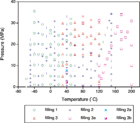
Temperature-pressure state points measured for the SRM toluene; the different symbols represent the different fillings.
The effect of dissolved air was investigated with a separate set of measurements carried out in May 2007. An abbreviated set of measurements with the original (degassed) sample covered the temperature range − 40 °C to 150 °C, with pressures to 32 MPa. Selected replicate measurements were made at − 40 °C to 50 °C in a separate filling. The density was measured at 51 temperature and pressure state points with an average of four repeat density determinations per state point, for a total of 216 p - ρ - T data points. The air-saturated sample was then measured at similar temperatures and pressures at 40 temperature and pressure state points for a total of 180 p - ρ - T data points. Following the measurements at 150 °C, the sample was cooled to 50 °C and measured again. The data for the degassed sample are given in Table A2 and the air-saturated data are given in Table A3 (see 7. Appendix A).
4.2. Estimated Fluid Density
The fluid density is represented using a 20-parameter empirical model
| (10) |
where T is temperature and p is pressure in MPa. (We use T to indicate temperatures in kelvins and t for temperatures in °C.) In fitting the model parameters, shown in Table 3, we excluded points with t < − 50 °C or t > 150 °C. The empirical model can be used to estimate the density for any temperature in the range of − 50 °C to 150 °C (223.15 K to 423.15 K) and any pressure in the range of 0.1 MPa to 30 MPa. The lower pressure limit represents a modest extrapolation of the experimental data; the upper pressure limit is conservative, since we used the data at p > 30 MPa in the fit. Table 4 gives values of ρ, calculated from Eq. (10) for even increments of temperature and pressure. Figure 5 displays the density measurements versus temperature and pressure that were used to fit the 20-parameter model.
Table 3.
Parameters for empirical model (Eq. 10)
| k | ak | bk | ck |
|---|---|---|---|
| 1 | 0.118 648 × 104 | 0 | 0 |
| 2 | −0.133 648 × 103 | −0.80 | 0 |
| 3 | −0.119 260 × 10−1 | −5.34 | 0 |
| 4 | 0.229 402 | −0.10 | 1.00 |
| 5 | 0.187 212 × 10−4 | −7.60 | 1.00 |
| 6 | 0.661 127 × 10−1 | −2.20 | 1.15 |
| 7 | −0.249 953 × 10−1 | −2.24 | 1.30 |
| 8 | −0.280 091 × 10−5 | −7.93 | 1.30 |
Table 4.
Estimated fluid density ρ in kg/m3 for degassed samples (g = 0 kg/m3) calculated from Eq. (10)
| t (°C) | 0.1 | Pressure (MPa) | |||||||
|---|---|---|---|---|---|---|---|---|---|
| 1 | 2 | 5 | 10 | 15 | 20 | 25 | 30 | ||
| −50 | 931.655 | 932.100 | 932.605 | 934.118 | 936.595 | 939.011 | 941.370 | 943.678 | 945.937 |
| −40 | 922.362 | 922.833 | 923.366 | 924.963 | 927.573 | 930.114 | 932.592 | 935.012 | 937.377 |
| −30 | 913.101 | 913.598 | 914.162 | 915.848 | 918.600 | 921.274 | 923.877 | 926.415 | 928.893 |
| −20 | 903.860 | 904.386 | 904.982 | 906.763 | 909.665 | 912.481 | 915.216 | 917.879 | 920.475 |
| −10 | 894.627 | 895.184 | 895.815 | 897.699 | 900.762 | 903.726 | 906.602 | 909.397 | 912.118 |
| 0 | 885.392 | 885.982 | 886.651 | 888.645 | 891.878 | 895.002 | 898.027 | 900.962 | 903.813 |
| 10 | 876.142 | 876.769 | 877.478 | 879.589 | 883.006 | 886.300 | 889.482 | 892.564 | 895.554 |
| 20 | 866.864 | 867.531 | 868.284 | 870.522 | 874.136 | 877.610 | 880.960 | 884.198 | 887.334 |
| 30 | 857.545 | 858.255 | 859.056 | 861.432 | 865.257 | 868.924 | 872.453 | 875.856 | 879.145 |
| 40 | 848.170 | 848.929 | 849.782 | 852.307 | 856.359 | 860.233 | 863.952 | 867.530 | 870.982 |
| 50 | 838.726 | 839.537 | 840.448 | 843.134 | 847.432 | 851.529 | 855.450 | 859.215 | 862.838 |
| 60 | 829.195 | 830.065 | 831.038 | 833.902 | 838.466 | 842.802 | 846.939 | 850.902 | 854.706 |
| 70 | 819.562 | 820.496 | 821.539 | 824.597 | 829.450 | 834.043 | 838.413 | 842.586 | 846.581 |
| 80 | 809.808 | 810.815 | 811.935 | 815.205 | 820.373 | 825.244 | 829.863 | 834.260 | 838.458 |
| 90 | 799.916 | 801.003 | 802.208 | 805.713 | 811.225 | 816.397 | 821.283 | 825.919 | 830.330 |
| 100 | 789.865 | 791.043 | 792.342 | 796.106 | 801.994 | 807.492 | 812.665 | 817.556 | 822.194 |
| 110 | 779.634 | 780.914 | 782.318 | 786.369 | 792.669 | 798.521 | 804.005 | 809.167 | 814.044 |
| 120 | * | 770.596 | 772.118 | 776.486 | 783.239 | 789.478 | 795.295 | 800.748 | 805.878 |
| 130 | * | 760.069 | 761.722 | 766.443 | 773.694 | 780.353 | 786.531 | 792.294 | 797.691 |
| 140 | * | 749.309 | 751.110 | 756.222 | 764.022 | 771.140 | 777.707 | 783.803 | 789.481 |
| 150 | * | 738.293 | 740.259 | 745.808 | 754.214 | 761.832 | 768.820 | 775.270 | 781.246 |
above the normal boiling point temperature (liquid phase not stable at p = 0.1 MPa)
Fig. 5.
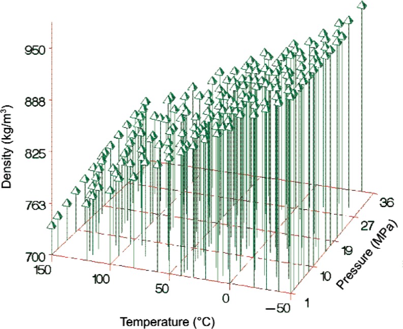
906 density measurements versus temperature and pressure used to develop the density model (Eq. 10).
4.3. Correction for Air-Saturated Samples
While the data used to fit the empirical model Eq. (10) were collected for degassed samples, the data measured at near-ambient conditions for the previous issue of this SRM were based on samples having some degree of air saturation. Thus, a correction Δ was added to the computed fluid density to align the near-ambient SRM and degassed data so that the estimated fluid density is
| (11) |
where
| (12) |
and Δ is a function of t and p.
The value Fair represents the fraction of air saturation and g is the estimated density correction in kg/m3. If measurements are based on degassed samples, then Fair = 0, and the correction Δ and its associated uncertainty are zero.
The density correction for air-saturated samples was determined from the supplemental density measurements for both air-saturated and degassed samples (as listed in Tables A2 and A3). Because measurements for air-saturated and degassed samples could not be made at exactly the same temperatures and pressures, a rational function of the form
| (13) |
was fitted to the air-saturated density measurements, and a similar model was fitted separately to the degassed density measurements ρdegassed. Next, the two rational functions were used to predict the density of each point in the combined air-saturated and degassed data sets. The predicted density correction is
| (14) |
where are the predicted densities based on each rational function.
We analyzed predicted corrections for pressures ranging from 0.1 MPa to 20 MPa and temperatures ranging from − 40 °C to 100 °C. The predicted correction surface for 228 different temperature and pressure combinations is shown in Fig. 6. We do not have a theoretical basis for selecting a functional form for the air-saturated density correction, and because this correction is only slightly larger than the uncertainties in the measured densities there is the danger of “over-fitting” with a strictly empirical function. Thus, we fitted a very simple temperature/pressure model
| (15) |
to the predicted corrections. Thus, the estimated correction for air-saturation is determined from
| (16) |
where t is in °C and p is in MPa. For example, the estimated density correction at 25 °C and 0.1 MPa is g = − 0.0628 kg/m3. This result is in excellent agreement with the value of − 0.062 kg/m3 ± 0.007 kg/m3 reported by Ashcroft and Isa [12] for degassed versus air-saturated toluene at similar conditions. Figure 7 displays the estimated correction surface for air-saturation based on Eq. (16) for selected temperatures and pressures. The correction is not reliable for pressures smaller than 0.1 MPa or larger than 20 MPa, and temperatures less than − 50 °C or greater than 100 °C.
Fig. 6.
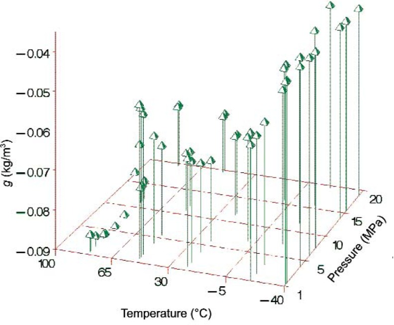
Density correction for air-saturated versus degassed toluene based on experimentally measured points.
Fig. 7.
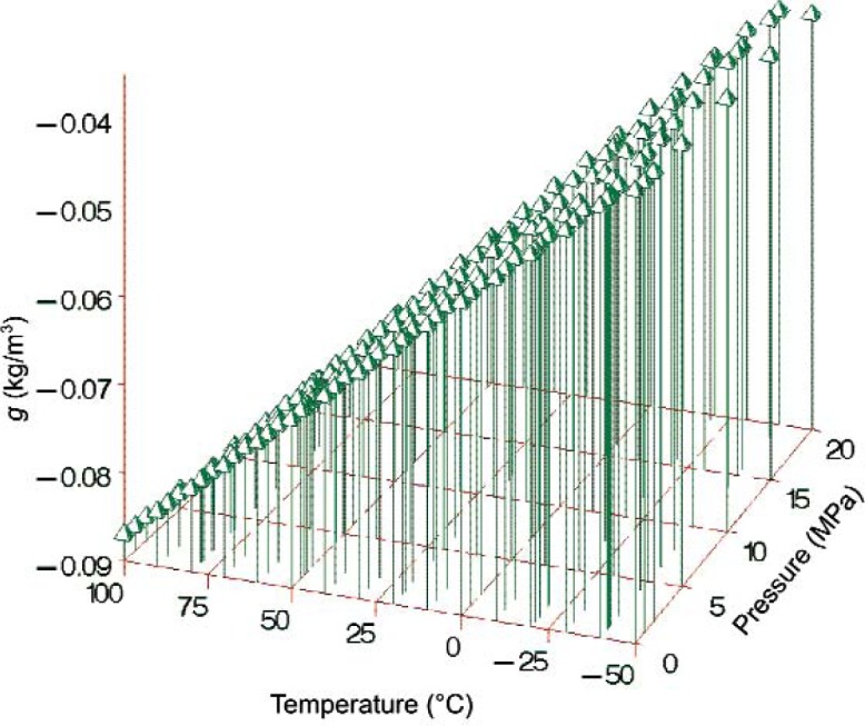
Estimated correction surface for air-saturated versus degassed toluene (Eq. 16).
We measured the air-saturated samples at temperatures up to 150 °C, but in fitting Eq. (16) we found that the trends in g with temperature and pressure became inconsistent at temperatures above 100 °C. We took this as evidence of decomposition and/or reaction of the toluene with oxygen at the higher temperatures. Thus, we fitted the correction only to the lower-temperature data. The lower temperature limit of − 50 °C for Eq. (16) represents a modest extrapolation of the experimental data.
The densities measured in May 2007 for the degassed toluene are, on average, 0.057 kg/m3 higher than the densities measured during January to March 2006. The 2006 measurements (which form the basis for the “official” SRM densities) were also made on the same (degassed) sample. This difference is larger than the standard uncertainty in the measured densities, although it is within the expanded uncertainty. The sample had been stored in the 2.5 L stainless steel sample cylinder in the 13 months between the two series of measurements. Storage in a metal container may result in more degradation of the sample, compared to storage in the glass SRM vials. There is also the possibility that the densimeter drifted by this amount. We carry out periodic measurements on high-purity argon to check for any such drifts, and we found no significant differences between argon measurements made in January 2005 and those made in June 2007.
5. Uncertainty Analysis
The overall uncertainty in the fluid density arises from several distinct sources. The first source is the empirical model used to represent the density and allow interpolation at a desired temperature and pressure. A second category relates to the material itself; these include uncertainties associated with the degree of air saturation of the toluene and possible degradation resulting from exposure to high temperatures. Since the SRM is provided in 5 mL ampoules (vials), the variation in density from vial to vial must also be considered. The third, and most complex, source arises from the experimental measurement of the density. Finally, when using the SRM for the calibration of a densimeter, the uncertainty in the user’s temperature and pressure measurement must be included.
According to accepted methods for determining uncertainty [13], the measurement equation is the starting point for estimating uncertainty. For practical purposes, our measurement equation is given by Eq. (11), however vial-to-vial effects (V), apparatus effects (e), material degradation effects (x), and errors in the user’s temperature and pressure measurements (tp) must also be included in the measurement equation even though their values are thought to be zero. The complete measurement equation is thus
| (17) |
where ρ represents the density estimate from the empirical model and Δ is the correction for air saturation. Although the values of V, x, e, and tp are thought to be zero, they still have some uncertainty.
The combined standard uncertainty, assuming independent input quantities, for the estimated fluid density ρC Eq. (17) is
| (18) |
where u(ρ) is the uncertainty associated with the empirical model, u(V) is the uncertainty associated with vial-to-vial variations (based on measurements carried out at near-ambient conditions), and u(x) is the uncertainty associated with any possible degradation (i.e., change in chemical composition) of the sample resulting from exposing it to high temperatures. The uncertainty associated with the “air-saturated” correction is u(Δ). If samples are degassed before taking measurements, then no correction is needed and u(Δ) = 0. The quantity u(e) is the uncertainty associated with a single experimental density measurement, which we can think of as a method/apparatus uncertainty. The final uncertainty component u(tp) represents the uncertainty associated with the user’s temperature and pressure measurements.
Details regarding the estimation of each of these uncertainty components are provided below.
5.1 Uncertainty u(ρ) Due to Empirical Model
Our best estimate of the uncertainty associated with the 20-parameter empirical model to fit density versus temperature and pressure is the root-mean-squared error of the fit, or
| (19) |
where n is the number of observations used in the fit, p is the number of parameters estimated, ρi denotes the i th observation of density, and ρfit is the fitted value associated with the i th observation. The value of u(ρ) is 0.0086 kg/m3 for our fit, and there are 906 − 20 = 886 degrees of freedom associated with u(ρ) (dfρ = 886).
5.2 Uncertainty u(Δ) Due to Air-Saturation of Samples
Based on the air-saturation correction equation Δ = Fair · g, the standard uncertainty associated with Δ (Eq. 12) is
| (20) |
obtained by use of propagation of errors techniques and by assuming that Fair and g are independent. The value of u(Δ) depends on both input quantities as well as their associated uncertainties. If the user is taking measurements on degassed samples, then Δ = 0 and u(Δ) = 0. The standard uncertainty associated with the correction g is u(g) = 0.0075 kg/m3, based on the worst-case prediction error associated with the model fit, i.e. Eq. (16). The degrees of freedom associated with u(g) are dfg = 224, based on 228 (t,p) data points and four model parameters.
The value of Fair for the SRM samples is estimated to be 0.59. We will assume the error in Fair is uniformly distributed within the interval 0.49 to 0.69 so that the standard uncertainty of Fair is
| (21) |
Assuming that the “uncertainty of the uncertainty” is 25 %, eight degrees of freedom are appropriate for the uncertainty due to Fair (dfFair = 8). (See equation G.3 of [13] for details regarding the degrees of freedom approximation.)
The degrees of freedom associated with u(Δ) are
| (22) |
based on the Welch-Satterthwaite approximation [13]. The values of Δ and u(Δ) for the SRM at (20 °C, 0.10 MPa, and Fair = 0.59) are Δ = − 0.0361 kg/m3 and u(Δ) = 0.0054 kg/m3 with dfΔ = 25.
5.3 Uncertainty u(V) Due to Vial-to-Vial Variability at Near-Ambient Conditions
The value of u(V) represents the combined vial-to-vial, day-to-day, and apparatus uncertainties at near-ambient conditions provided in the previous SRM report of analysis [4]. This analysis involved using a vibrating-tube densimeter to compare the density of samples from randomly selected 5 mL ampoules with the toluene used in the hydrostatic apparatus described by Bean and Houser [4]. The three sources of uncertainty included in u(V), and their degrees of freedom, are listed in Table 5 for convenience. The value of u(V) = 0.0114 kg/m3 was determined by adding the three sources in quadrature and taking the square root of the sum. The degrees of freedom, dfV = 32, were calculated with the Welch-Satterthwaite approximation. We assume that u(V) is the same for all temperatures and pressures.
Table 5.
Uncertainty and degrees of freedom associated with vial-to-vial variability at near-ambient conditions (from Bean and Houser [4])
| Source | Uncertainty (kg/m3) | Degrees of Freedom |
|---|---|---|
| Apparatus | u (A) = 0.0032 | dfA = ∞ |
| Day-to-day | u (D) = 0.0047 | dfD = 5 |
| Ampoule-to-ampoule | u (v) = 0.0099 | dfv = 23 |
|
| ||
| Total | u (V) = 0.0114 | dfV = 32 |
5.4 Uncertainty Due to Material Degradation and Time u(x)
Replicate measurements collected at 40 °C at the completion of a filling were used to determine the uncertainty due to material degradation and time effects. Any degradation in the toluene would be expected to be a function of both time and temperature (a short time at a high temperature would yield degradation similar to that resulting from a prolonged exposure to a moderate temperature). This term is also confounded with any possible drift in the experimental apparatus with time. While repeat measurements for a target temperature are easily obtained, target pressures are more difficult to achieve, and thus the pressures vary among the replicates. Figure 8 displays measurements taken at 40 °C over the course of this study.
Fig. 8.

Replicate measurements at 40 °C for the various fillings of toluene.
A fourth-order polynomial was fitted to the “complete” 40 °C isotherm for the filling #2 data in Fig. 8; these measurements were made before the sample was exposed to higher temperatures. The residuals from the fit are shown in Fig. 9. The data from other fillings provide information about how the material may have changed over time and/or with exposure to high temperatures. The residuals indicate that the data from the other fillings are similar to the filling #2 data, with the exception of the filling #1 measurements at about 22 MPa. We will assume that the largest residual (conservatively estimated at 0.006 kg/m3) represents the worst-case error that might be observed. If the worst-case error is also assumed to represent the bounds of a uniform distribution, (− 0.006 kg/m3, 0.006 kg/m3) we can approximate the uncertainty due to material degradation and time effects as
| (23) |
Fig. 9.

Residuals from the polynomial fit to filling #2 data at 40 °C; the plot symbols are the same as in Fig. 8.
This uncertainty is assumed to be valid for all temperatures included in this study. Assuming that the “uncertainty of the uncertainty” is 25 %, eight degrees of freedom are appropriate for the uncertainties due to material degradation and time errors (dfx = 8).
5.5 Uncertainty u (e) Due to Method/Apparatus
To estimate u (e) for given values of temperature (°C) and pressure (MPa), the polynomial equation
| (24) |
was fitted to values of the uncertainty associated with each measurement of fluid density across the temperature-pressure surface. Details regarding the computation of the uncertainty of fluid density measurements u (ρfluid) are discussed in the sections that follow. The quantity u (e) denotes the uncertainty predicted by the polynomial based on the values of u (ρfluid) computed for each data point. The error introduced into u (e) by using the polynomial equation is negligible compared to the magnitude of u (e). The degrees of freedom associated with u (ρfluid) vary depending on pressure and temperature, and range from 9 to 18. Thus, a conservative estimate for the degrees of freedom associated with u (e) is 9 (dfe = 9).
5.5.1 Uncertainty u(ρfluid) in Fluid Density Measurements
As discussed in Sec. 2, the experimental fluid density data were calculated with Eqs. (2 to 5). The uncertainty of a single fluid density measurement, ρfluid, thus, is a function of the 14 input quantities:
| (25) |
Many of the 14 input quantities are, in turn, dependent upon other measured quantities.
The values of u (ρfluid) computed for each data point will be used to determine the parameters of a polynomial to predict uncertainty for a given temperature and pressure. The predicted uncertainty, u(e), represents the method/apparatus error. Based on propagationof errors techniques, assuming that all the input quantities are independent, the variance of ρfluid is
| (26) |
and the combined standard uncertainty is the square root of the variance.
The Welch-Satterthwaite approximation [13] was used to estimate the degrees of freedom associated with u (ρfluid):
| (27) |
where
| (28) |
and Ψi represents each of the 14 input variables in Eq. (25). The derivatives in u (ρfluid) and dffluid are quite complicated, so we used a commercial symbolic algebra software package to generate the derivatives.
Next, we will provide details regarding the estimation of each individual component of uncertainty and its associated degrees of freedom.
5.5.2 Uncertainties u (mcal), u (mtare), u (m1), and u (m2) in Masses
A single measurement of the mass of an unknown object, mxi, is determined by comparison to standard masses using a “SXXS” method (with S referring to a standard and X the unknown). By this method the mass of the unknown is given by
| (29) |
where the Oi are the balance readings, the ms and msw are standard masses, and ρs and ρsw are the densities of the standard masses. This method is described as “Standard Operating Procedure 4” by Harris and Torres [5]. We need to estimate the mass and the uncertainty of the mass for two sinkers, m1 and m2. We will assume the uncertainties associated with the calibration masses mcal and mtare are the same as those for m1 and m2.
Propagation of errors was used to determine the uncertainty associated with a single mass measurement. Assuming all input quantities are independent, the variance of the unknown mass is
| (30) |
and the combined standard uncertainty of the unknown mass is u (mxi) = [u2(mxi)]0.5.
Next, we describe the evaluation of each individual uncertainty component in the mass determination. Table 6 displays information for the standard masses provided by their manufacturer’s calibration laboratory. Since the nominal value of ms = 60 g is obtained by use of the 50 g and 10 g standards together, the uncertainty of ms is
| (31) |
Table 6.
Calibration data for the standard masses used in this work
| Nominal Mass (g) |
True Mass (g) |
Uncertainty (g) |
Density (g/cm3) |
|---|---|---|---|
| 50 | 50.000 1507 | 0.000 011 45 | 7.85 |
| 10 | 9.999 9966 | 0.000 008 15 | 7.85 |
| 2 | 2.000 0193 | 0.000 0032 | 7.85 |
The nominal value of msw is 2 g, so u (msw) = 0.000 0032 g. We believe the errors associated with the density of the standard masses are best described by a uniform distribution bounded by 0.05 g/cm3. Thus standard uncertainties of ρs and ρsw are
| (32) |
We know from the analysis of the sinker volume determination (Secs. 3.3 and 5.5.4) that the standard uncertainties associated with the densities of m1 and m2 used in our experiment are u (ρx) = 0.000 11 g/cm3 for the density of sinker 1 (titanium) and u (ρx) = 0.000 42 g/cm3 for the density of sinker 2 (tantalum). The repeatability standard deviation of the balance is 0.03 mg or 0.000 03 g, so the standard uncertainties of the observed balance readings are u (O1) = u (O2) = u (O3) = u (O4) = 0.000 03 g.
A single determination of the density of moist air, ρair, was computed using the function of Davis [6], which is ultimately a function of temperature (t), pressure (p), and relative humidity (h). Using propagation of errors, and assuming independence of input quantities, the combined standard uncertainty of a single measurement of ρair is
| (33) |
For a single determination of air density, the standard uncertainties for temperature, pressure, and humidity are u (t) = 0.2 K, u (p) = 0.0001 ⋅ p kPa, and u (h) = 0.02.
The value u (mxi) is the uncertainty associated with a single mass determination. The nominal mass values used in the density calculations are averages based on six repeat measurements (three measurements on each of two days), so we need to determine the uncertainty of the average mass.
Typically we would use the six repeat measurements to determine the uncertainty of the average mass value; however, a more extensive repeatability study was performed over four days with three repeated measurements per day. Thus, we will estimate the uncertainty of the average mass using the larger, more comprehensive data set and assume the uncertainty will be the same for the six measurements actually used. There appears to be no significant between-day effect for either sinker based on an analysis of variance, so we were able to combine all data and ignore the fact that the measurements were taken on different days.
We need to estimate two sources of variation—within measurements and between measurements—from the larger repeatability study in order to compute the uncertainty of the average mass. The within-measurement variance was computed as the average variance of the 12 repeated measurements,
| (34) |
The values of u 2(mxi) were computed as described earlier in this section. The between-measurement variance is computed as the variance of the 12 mass measurements
| (35) |
Assuming the within-measurement and between-measurement variation based on the larger repeatability study are the same for the six measurements actually used in the experiment, the uncertainty of the average mass based on six observations is
| (36) |
The estimated uncertainties for sinker 1 and sinker 2 are u (m1) = 0.000 021 g and u (m2) = 0.000 023 g, and each uncertainty estimate has 6 − 1 = 5 degrees of freedom (dfm1 = dfm2 = 5).
The values of mcal and mtare were estimated in a similar fashion; however, there is only one determination of each mass, and u (mcal) = u (mtare) = 0.000 050 g. Because there is only one observation for mcal and mtare, we will use engineering judgment to determine the degrees of freedom associated with u (mcal) and u (mtare). Assuming that the “uncertainty of the uncertainty” is 50 %, there are two degrees of freedom associated with each uncertainty estimate (dfmcal = dfmtare = 2).
5.5.3 Uncertainties u (Vcal) and u (Vtare) in Volumes of the Calibration Masses
The limits to error of Vcal and Vtare were estimated to be 0.05 % of the nominal sinker volume based on engineering judgment. Assuming the limits represent a uniform distribution, the standard uncertainties associated with Vcal and Vtare are
| (37) |
We determined that eight degrees of freedom were appropriate based on the assumption that the “uncertainty of the uncertainty” is 25 % (dfVcal = dfVtare = 8).
5.5.4 Uncertainty u (V1) and u (V2) in Sinker Volumes
The determination of the sinker volumes involves the determination of their volumes at 20 °C and atmospheric pressure by the hydrostatic experiment described in Sec. 3.3. These values must then be adjusted for the effects of temperature and pressure. Each of these components involves multiple sources of uncertainties.
5.5.4.1 Uncertainty u (Vref) in Sinker Volumes at 20 °C
A summary of the uncertainties contributing to the sinker volume uncertainty at the reference temperature of 20 °C is presented in Table 7. The uncertainty in the density of the silicon standards is that assigned by the NIST Mass Group [9]. The uncertainty in the mass determinations of the standards and sinkers includes the balance linearity, uncertainty in the calibration masses, uncertainty in air buoyancy, and possible surface adsorption of water. For the hydrostatic weighings, the effects of the balance calibration and linearity are reduced because of the relatively small weight differences measured. Air buoyancy and surface adsorption do not apply. (The sinkers were immersed in the fluid for more than 48 hours prior to the volume determination, giving them time to come to equilibrium with the fluid.) However, the hydrostatic weighings were affected by an observed linear drift of 0.0003 g/h, as determined by the drift in the pan weighings taken every 16 minutes over the course of the test. The largest deviation from the linear trend was 0.000 12 g, with an average of less than 0.000 05 g.
Table 7.
Summary of standard uncertainties in volumes determined by hydrostatic weighing
| Source of Error | Magnitude of Error | Sinker 1 (Ti) | Uncertainty in Volume (cm3) | Ta ref to Ti | |
|---|---|---|---|---|---|
| Sinker 2 (Ta) | Si ref to Si | ||||
| Density of standard | 1.6 × 10⁻⁵ g/cm3 | 9.15 × 10⁻⁵ | 2.48 × 10⁻⁵ | 29.2 × 10⁻⁵ | 2.66 × 10⁻⁵ |
| Mass of standard | 5.0 × 10⁻⁵ g | 0.29 × 10⁻⁵ | 0.80 × 10⁻⁵ | 0.92 × 10⁻⁵ | 0.53 × 10⁻⁵ |
| Mass of object | 5.0 × 10⁻⁵ g | 3.07 × 10⁻⁵ | 3.07 × 10⁻⁵ | 3.07 × 10⁻⁵ | 3.07 × 10⁻⁵ |
| Weighing of standard | 5.0 × 10⁻⁵ g | 0.96 × 10⁻⁵ | 0.26 × 10⁻⁵ | 3.07 × 10⁻⁵ | 0.83 × 10⁻⁵ |
| Weighing of object | 5.0 × 10⁻⁵ g | 3.07 × 10⁻⁵ | 3.07 × 10⁻⁵ | 3.07 × 10⁻⁵ | 3.07 × 10⁻⁵ |
|
| |||||
| Root-sum-of-squares | 10.2 × 10⁻⁵ | 5.07 × 10⁻⁵ | 29.7 × 10⁻⁵ | 5.19 × 10⁻⁵ | |
The effects of the error sources on the calculated volumes are given for four cases. The columns labeled “Sinker 1 (Ti)” and “Sinker 2 (Ta)” are for the two sinkers, where the silicon standards were taken as the knowns, i.e., the ratios AB, CB, and BC for the Ta sinker and the ratios AD, DA, DC, and CD for the Ti sinker. The column “Si ref to Si” is for the check measurement comparing one silicon standard to the other (the ratio AC). “Ta ref to Ti” is for the calculation of the tantalum sinker volume taking the titanium sinker volume as the known (the ratio DB). The overall uncertainty varied from 0.000 0052 cm3 to 0.000 030 cm3, with objects having the highest density (i.e., the smallest volume and buoyancy force) having the highest relative uncertainties.
The measured volumes of the two sinkers at the reference temperature V1ref and V2ref have uncertainties due to both random and systematic effects. The standard uncertainties associated with random errors, from a least-squares analysis of the hydrostatic data, are u (V1R) = 0.000 0023 cm3 and u (V2R) = 0.000 0031 cm3. There are six degrees of freedom associated with each estimate (dfV1R = dfV2R = 6). The standard uncertainties associated with systematic calibration effects are u (V1S) = 0.000 102 cm3 and u (V2S) = 0.000 050 cm3. Assuming that the “uncertainty of the uncertainty” is 25 %, eight degrees of freedom are appropriate for the uncertainties due to systematic effects (dfV1S = dfV2S = 8).
Thus, the combined standard uncertainty of the volume of sinker 1 at reference conditions (20 °C and 0.08 MPa) is
| (38) |
and the degrees of freedom are given by
| (39) |
Similar equations were used to determine the combined standard uncertainty and degrees of freedom for the measured volume of sinker 2.
5.5.4.2 Uncertainty in Sinker Volumes u (V1) and u (V2) as a Function of T and p
The volumes of sinker 1 (Ti) and sinker 2 (Ta) determined by the hydrostatic comparator experiment at 20 °C (V1ref and V2ref) must be modified by three additional corrections to account for temperature and pressure effects:
| (40) |
where Vκ accounts for pressure effects and Vα and VT account for temperature effects (i.e., thermal expansion).
The combined standard uncertainties for the volumes of the sinkers, based on propagation of errors and independent input quantities, are given by
| (41) |
The uncertainty of the temperature correction VT also includes uncertainty of the Vα correction (as discussed below), so u (Vα) does not appear in the uncertainty calculation. The degrees of freedom associated with u (V1) are
| (42) |
A similar equation is used to compute dfV2.
The correction, Vκ, is defined as
| (43) |
where κ0 is the bulk modulus of the sinker material. The uncertainties of the two pressures are negligible compared to the uncertainty of κ0. Thus, the standard uncertainty of Vκ is
| (44) |
where u (κ0) = 0.05 ⋅ κ0, based on engineering judgment. The value of κ0 for titanium is 108.4 × 10⁶ GPa−1 and the value for tantalum is 196.3 × 10⁶ GPa−1 [14]. Assuming that the “uncertainty of the uncertainty” is 25 %, 8 degrees of freedom were appropriate (dfVκ = 8).
Because volume measurements were taken at a nominal temperature of 20 °C, we need to correct the volume of the sinkers for density measurements taken at other temperatures. Vα is a correction based on measured values of the thermal expansion of the titanium and tantalum used to fabricate the sinkers (see [1]).
VT is an additional calibration based on measurements of low-pressure (i.e., nearly ideal) gases in the two-sinker densimeter. Gas densities were measured at several (nearly identical) pressures along several isotherms. The densities at corresponding pressures along pairs of isotherms were ratioed and extrapolated to zero pressure, where the ideal-gas law applies:
| (45) |
where Tref is the temperature (293.15 K) of the hydrostatic sinker volume determination. The basic concept is that of a gas thermometer, except inverted (i.e., the temperatures are the known quantities and the densities are the unknown quantities, rather than vice versa). The difference (in percent) between the extrapolated density ratio and the measured temperature ratio for a given pair of isotherms is the percentage adjustment in the sinker volumes resulting from this calibration. The results are summarized in Fig. 10 for these calibrations on three different gases. (See McLinden [15] for a complete discussion of this calibration, its uncertainties, and a listing of the data.)
Fig. 10.
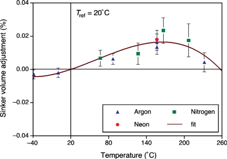
Sinker volume adjustment as a function of temperature based on measurements of low-density gases (adapted from McLinden [15]). The reference temperature for the adjustment is 20.00 °C, and the error bars represent standard uncertainties.
We used weighted least-squares regression to fit a cubic polynomial, which was constrained to pass through zero at the reference temperature of 20 °C, to the sinker volume adjustment data. A quadratic equation based on the standard uncertainties given by McLinden [15] (and shown by the error bars in Fig. 10) was used as the weighting function for the regression analysis. The weighted regression equation was used to estimate VT, and the standard uncertainty of VT is the standard error of a predicted VT. Both VT and u (VT) depend on the temperature; values of VT range from − 0.0036 % to 0.0163 % of the sinker volume, and values of u (VT) range from 0.0021 % to 0.0105 %. Since 11 observations and three model parameters were used in the fit, there are 8 degrees of freedom associated with u (VT) (dfVT = 8).
The VT calibration was applied to sinker volume data that include the Vα correction, and any error in Vα will result in a different value for the VT calibration. Indeed, the entire purpose of the VT calibration is to improve upon the Vα correction. This is why u (Vα) does not appear in Eqs. (41) and (42).
5.5.5 Uncertainty in Purge Gas Density u (ρN2)
The density of the nitrogen purge gas in the balance chamber was computed with a virial expansion
| (46) |
where Wm is the molar mass, R is the molar gas constant, and the second virial coefficient B is a function of temperature given by Span et al. [16]. The estimated uncertainty in the nitrogen density calculated by Eq. (46) at the near-ambient conditions of interest here is less than 0.01 %. The combined standard uncertainty of the density of nitrogen, u (ρN2), is a function of pressure and temperature, so that
| (47) |
with degrees of freedom
| (48) |
We need to determine u (T), u (p), dfT, and dfp to calculate u (ρN2) and dfN2. Each of the uncertainties u (T) and u (p) has a random component since we use the average of six repeat measurements in each density calculation. The uncertainties also have systematic components that are given by the standard uncertainties 0.2 K for temperature and 0.01 % for pressure. The combined standard uncertainties for temperature and pressure are
| (49) |
and
where ST and Sp are standard deviations in the six temperature and pressure readings, respectively. There are five degrees of freedom associated with each random component. Assuming the “uncertainty of the uncertainty” of each systematic component is 25 %, based on engineering judgment, there are eight degrees of freedom associated with each systematic component. The degrees of freedom for u (T) and u (p) can be computed from the Welch-Satterthwaite approximation, as follows:
| (50) |
| (51) |
5.5.6 Uncertainty u (Wcal), u (Wtare), u (W1), and u (W2) in Weighings
The values of Wcal, Wtare, W1, and W2 are all averages of ten measurements, so the estimated standard uncertainties of the four weighings are
| (52) |
Each uncertainty has 9 degrees of freedom (dfWcal = dfWtare = dfW1 = dfW2 = 9).
5.5.7 Uncertainty u (ρ0) in Apparatus Zero
Zero pressure (or vacuum) density readings were collected between toluene fillings to provide an indication of the amount of drift in the measurement system over time. The vacuum data were collected in the following sequence:
vacuum data “A”: January 5, 2006
toluene filling #1
vacuum data “B": January 20, 2006
vacuum data “C”: February 1, 2006
toluene fillings #2 and 2a
vacuum data “D”: February 24, 2006
toluene fillings #3, 3a, and 3b
vacuum data “E”: March 11, 2006.
Four separate straight-line regression equations were fit to consecutive pairs of vacuum measurements. For example, a straight line fit to vacuum data A and vacuum data B would be used to estimate the amount of drift for measurements taken during toluene filling #1. Thus, the regression equations depend on the elapsed time from the start of the experiment to the measurement of interest. The estimated density ρ0 for a measurement taken at elapsed time τ0 is
| (53) |
where c0 and c1 are fitting parameters, and the standard uncertainty of ρ0 is
| (54) |
where n is the number of observations used to estimate the regression line and s is the standard deviation of the fit. There are n − 2 degrees of freedom associated with u (ρ0) (dfρ0 = n − 2).
5.5.8 Summary of u (ρfluid)
Table 8 displays two examples of calculations of u (ρfluid) for density determinations near ambient conditions (t = 20 °C and p = 1.0 MPa, Table 8a) and for more extreme conditions (t = 150 °C and p = 30 MPa, Table 8b). Since there are multiple observations at the selected temperature and pressure combinations, the values in the table represent average uncertainties and sensitivity coefficients. The information in the table provides some insight into the role of the magnitude of the uncertainty and sensitivity coefficient for each source of uncertainty. Table 8 considers only the apparatus/method uncertainties and their associated degrees of freedom; they are a subset of the overall combined uncertainty discussed in Sec. 5.7.
Table 8a.
Uncertainty “budget” for ρ fluid (Eq. 26) for two sets (a, b) of operating conditions. The sensitivity coefficients have been multiplied by 1000 to convert to kg/m3
| Source |
t = 20 °C, p = 1 MPa
|
|||
|---|---|---|---|---|
| Standard Uncertainty | Sensitivity Coefficient |
ci ⋅ u (xi) (kg/m3) |
Degrees of Freedom | |
| u (xi) | ci | |||
| Wcal | 2.557 × 10⁻⁷ g | 42.039 | 1.075 × 10⁻⁵ | 9 |
| Wtare | 2.131 × 10⁻⁷ g | 56.478 | 1.203 × 10⁻⁵ | 9 |
| mcal | 5.000 × 10⁻⁵ g | 42.041 | 2.102 × 10⁻³ | 2 |
| mtare | 5.000 × 10⁻⁵ g | 56.481 | 2.824 × 10⁻³ | 2 |
| Vcal | 2.159 × 10⁻³ cm3 | 0.039 | 8.362 × 10⁻⁵ | 8 |
| Vtare | 2.159 × 10⁻³ cm3 | 0.053 | 1.142 × 10⁻⁴ | 8 |
| ρair | 6.295 × 10⁻⁷ g/cm3 | 107.996 | 6.799 × 10⁻⁵ | 8 |
| m1 | 2.100 10−5 × g | 97.345 | 2.044 × 10⁻³ | 5 |
| m2 | 2.300 × 10⁻⁵ g | 82.905 | 1.907 × 10⁻³ | 5 |
| V1 | 3.161 × 10⁻⁴ g | 84.451 | 2.670 × 10⁻² | 9 |
| V2 | 9.513 × 10⁻⁵ g | 71.924 | 6.842 × 10⁻³ | 13 |
| W1 | 1.832 × 10⁻⁶ g | 97.342 | 1.784 × 10⁻⁴ | 9 |
| W2 | 3.967 × 10⁻⁷ g | 82.903 | 3.289 × 10⁻⁵ | 9 |
| ρ0 | 4.402 × 10⁻⁹ 3 g/cm | 1000.0 | 4.402 × 10⁻⁶ | 48 |
Although there are 14 individual sources of uncertainty in u (ρfluid), not all sources contribute a significant amount to the total uncertainty. We selected a few temperature and pressure combinations and computed the percentage of the total variation for all 14 sources of uncertainty. Table 9 displays the percentage of total variation for the top six contributing sources as well as the combined percentage of the remaining eight sources and the value of u (ρfluid). Again, the values in the table represent average percentages and the average uncertainties. The largest contributor to u (ρfluid) for all temperature and pressure combinations is u (V1), the uncertainty in the volume of the titanium sinker, followed by u (V2), the volume of the tantalum sinker. These two sources of uncertainty account for 98 % to 99 % of the total variation in ρfluid.
Table 9.
Percentages of total variation in u (ρfluid) for six sources of uncertainty at various temperatures and pressures. The column labeled “all others” contains the combined percentage of total variation for the remaining eight sources. The value of u (ρfluid) is also listed. The quantities in the table represent average values for the given temperatures and pressures
|
t (°C) |
p (MPa) |
Percent of Total Variation
|
u (ρfluid) (kg/m3) |
||||||
|---|---|---|---|---|---|---|---|---|---|
| V1 | V2 | mcal | mtare | m1 | m2 | all others | |||
| −50 | 1 | 92.7 | 5.6 | 0.4 | 0.7 | 0.3 | 0.3 | 0.0 | 0.036 |
| −50 | 15 | 93.0 | 5.4 | 0.4 | 0.7 | 0.3 | 0.3 | 0.0 | 0.037 |
| 0 | 1 | 91.0 | 6.1 | 0.6 | 1.2 | 0.6 | 0.5 | 0.0 | 0.027 |
| 0 | 15 | 91.7 | 5.7 | 0.6 | 1.1 | 0.5 | 0.4 | 0.0 | 0.028 |
| 50 | 1 | 92.1 | 5.8 | 0.4 | 0.8 | 0.4 | 0.4 | 0.0 | 0.031 |
| 50 | 15 | 92.5 | 5.6 | 0.4 | 0.7 | 0.4 | 0.4 | 0.0 | 0.032 |
| 50 | 30 | 93.4 | 5.0 | 0.4 | 0.6 | 0.3 | 0.3 | 0.0 | 0.035 |
| 100 | 1 | 93.0 | 5.7 | 0.3 | 0.5 | 0.3 | 0.3 | 0.0 | 0.037 |
| 100 | 15 | 93.3 | 5.5 | 0.3 | 0.5 | 0.3 | 0.2 | 0.0 | 0.039 |
| 150 | 1 | 93.4 | 5.6 | 0.2 | 0.3 | 0.2 | 0.2 | 0.0 | 0.042 |
| 150 | 15 | 93.6 | 5.5 | 0.2 | 0.3 | 0.2 | 0.2 | 0.0 | 0.044 |
| 150 | 30 | 93.9 | 5.2 | 0.2 | 0.3 | 0.2 | 0.2 | 0.1 | 0.046 |
5.6 Uncertainty in Temperature and Pressure u (tp)
Since the fluid density is a function of temperature and pressure, uncertainties in the measured temperature and pressure will contribute to the uncertainty of the reported density. A sensitivity study was used to estimate u (tp) in which temperature and pressure were varied in Eq. (10) according to their corresponding uncertainty levels. The uncertainty u (tp) was determined from the resulting density values. For the present measurements u (t) = 0.002 °C and u (p) = 2 kPa, so that u (tp) = 0.0025 kg/m3. Assuming that the “uncertainty of the uncertainty” is 25 %, eight degrees of freedom are appropriate for this uncertainty (dftp = 8). The very small magnitude of this effect is a result of the nearly-incompressible nature of toluene over the temperatures and pressures studied. This effect would be much more significant if the present apparatus were used for measurements on a gas or a fluid near its critical point.
When this SRM is used in the calibration of a densimeter, u (tp) depends on the user’s temperature and pressure errors. Since each user’s measurement apparatus is different, we performed a sensitivity study for this uncertainty by varying temperature and pressure according to nine different combinations of error levels and quantifying the effect on density. The results of the sensitivity study are shown in Table 10. The error values listed in the first two columns of Table 10 represent a user’s limits to error (rather than a standard uncertainty), and the values of u (tp) are typical uncertainties across all temperatures and pressures in the test region. Ultimately, the user is responsible for estimating an appropriate value of u (tp) and its associated degrees of freedom.
Table 10.
Estimated uncertainty u (tp) due to user’s temperature and pressure uncertainties
| Limit to Temperature Error (°C) |
Limit to Pressure Error (MPa) |
u (tp) (kg/m3) |
|---|---|---|
| ± 0.001 | ± 0.001 | 0.001 |
| ± 0.01 | 0.005 | |
| ± 0.1 | 0.051 | |
| ± 0.01 | ± 0.001 | 0.005 |
| ± 0.01 | 0.007 | |
| ± 0.1 | 0.051 | |
| ± 0.1 | ± 0.001 | 0.053 |
| ± 0.01 | 0.054 | |
| ± 0.1 | 0.075 |
5.7 Combined Standard Uncertainty
The combined standard uncertainty associated with an estimated fluid density is given by Eq. (17). The values of u (ρ), u (V), and u (x) are constant for all temperature and pressure combinations. The value of u (e) depends on the operating temperature and pressure and is calculated from Eq. (24). The value of u (Δ) depends on the degree of air saturation in the measured sample (for degassed samples, u (Δ) = 0), and u (tp) depends on the level of error associated with the operating temperature and pressure in the user’s apparatus.
The values of the individual uncertainty components for the measurements described in this work are displayed along with their associated degrees of freedom in Table 11. Table 12 displays the combined standard uncertainty for four of the uncertainty components, u (ρ), u (V), u (x) and u (e) (from Table 11 and Eq. 24) for the same even increments of temperatures and pressures listed in Table 4.
Table 11.
Uncertainties and degrees of freedom for measurements described in this document *
| Source | Uncertainty (kg/m3) | Degrees of Freedom |
|---|---|---|
| u (ρ) | 0.0086 | 886 |
| u (V) | 0.0114 | 32 |
| u (x) | 0.003 | 8 |
| u (tp) | 0.002 47 | 8 |
Degassed samples only (u (Δ) = 0).
Table 12.
Combined standard uncertainty u in kg/m3, including the effects of u (ρ), u (V), and u (x) and u (e)
| t (°C) | 0.1 | Pressure (MPa) | |||||||
|---|---|---|---|---|---|---|---|---|---|
| 1 | 2 | 5 | 10 | 15 | 20 | 25 | 30 | ||
| −50 | 0.038 | 0.038 | 0.038 | 0.039 | 0.039 | 0.040 | 0.040 | 0.041 | 0.042 |
| −40 | 0.035 | 0.035 | 0.035 | 0.035 | 0.036 | 0.036 | 0.037 | 0.038 | 0.039 |
| −30 | 0.033 | 0.033 | 0.033 | 0.033 | 0.034 | 0.034 | 0.035 | 0.036 | 0.037 |
| −20 | 0.031 | 0.031 | 0.031 | 0.032 | 0.032 | 0.033 | 0.033 | 0.034 | 0.035 |
| −10 | 0.031 | 0.031 | 0.031 | 0.031 | 0.031 | 0.032 | 0.033 | 0.034 | 0.035 |
| 0 | 0.030 | 0.030 | 0.031 | 0.031 | 0.031 | 0.032 | 0.032 | 0.033 | 0.034 |
| 10 | 0.031 | 0.031 | 0.031 | 0.031 | 0.031 | 0.032 | 0.033 | 0.034 | 0.035 |
| 20 | 0.031 | 0.031 | 0.031 | 0.031 | 0.032 | 0.033 | 0.033 | 0.034 | 0.035 |
| 30 | 0.032 | 0.032 | 0.032 | 0.032 | 0.033 | 0.033 | 0.034 | 0.035 | 0.036 |
| 40 | 0.033 | 0.033 | 0.033 | 0.033 | 0.034 | 0.034 | 0.035 | 0.036 | 0.037 |
| 50 | 0.034 | 0.034 | 0.034 | 0.034 | 0.035 | 0.036 | 0.036 | 0.037 | 0.038 |
| 60 | 0.035 | 0.035 | 0.035 | 0.036 | 0.036 | 0.037 | 0.037 | 0.038 | 0.039 |
| 70 | 0.037 | 0.037 | 0.037 | 0.037 | 0.037 | 0.038 | 0.039 | 0.040 | 0.041 |
| 80 | 0.038 | 0.038 | 0.038 | 0.038 | 0.039 | 0.039 | 0.040 | 0.041 | 0.042 |
| 90 | 0.039 | 0.039 | 0.039 | 0.039 | 0.040 | 0.040 | 0.041 | 0.042 | 0.043 |
| 100 | 0.040 | 0.040 | 0.040 | 0.040 | 0.041 | 0.041 | 0.042 | 0.043 | 0.044 |
| 110 | 0.041 | 0.041 | 0.041 | 0.041 | 0.042 | 0.042 | 0.043 | 0.044 | 0.045 |
| 120 | * | 0.042 | 0.042 | 0.042 | 0.043 | 0.043 | 0.044 | 0.045 | 0.046 |
| 130 | * | 0.043 | 0.043 | 0.043 | 0.044 | 0.044 | 0.045 | 0.046 | 0.047 |
| 140 | * | 0.044 | 0.044 | 0.044 | 0.044 | 0.045 | 0.046 | 0.047 | 0.048 |
| 150 | * | 0.044 | 0.045 | 0.045 | 0.045 | 0.046 | 0.047 | 0.048 | 0.049 |
above the normal boiling point temperature (liquid phase not stable at p = 0.1 MPa)
5.8 Expanded Uncertainty and Degrees of Freedom
The expanded uncertainty is U = kuC, where the coverage factor k is obtained from the Student’s t distribution based on the effective degrees of freedom for uC. In general, the expanded uncertainty associated with a 100 · (1 − α) % coverage probability (α is 0.05 for 95 % coverage) is given by . Typically, k = 2 is used to compute the expanded uncertainty associated with a 95 % uncertainty interval. However, if the effective degrees of freedom are less than 30, the interval coverage is less than 95 %. Thus, we recommend that the effective degrees of freedom be computed to determine the proper coverage factor.
The effective degrees of freedom obtained from the Welch-Satterthwaite approximation are
| (55) |
Since the effective degrees of freedom depend on the value of u (e) for a given temperature and pressure, we will provide a conservative estimate of dfeff for all degassed measurements given in this document. The smallest (most conservative) value of dfeff is observed when u (e) is large since all other uncertainty sources and degrees of freedom are fixed. We used the largest value of u (e) observed for our data, u (e) = 0.053 kg/m3 (dfe = 9), and the remaining uncertainties and associated degrees of freedom from Table 11 to compute dfeff. Thus, a conservative value for all degassed measurements reported in this document is dfeff = 10, and the appropriate coverage factor for a 95 % uncertainty interval is 2.228.
When the SRM is used to calibrate a user’s densimeter, two of the uncertainty components of uC, ie. u (Δ) and u (tp), depend on the user’s conditions, so the final value of the user’s dfeff cannot be calculated in this document.
5.9 Uncertainty Example
We shall estimate the density and its uncertainty at t = −23 °C and p = 12 MPa for a degassed sample (Δ = 0 kg/m3 and u (Δ) = 0 kg/m3). The values of temperature and pressure are input into Eq. (10), resulting in a density estimate of 913.461 kg/m3. Similarly, u (e) = 0.0292 kg/m3 is calculated from Eq. (24). If the limit to temperature error is thought to be ± 0.1 °C, and the limit to pressure error is ± 0.1 MPa, then from Table 10, u (tp) = 0.075 kg/m3. The combined standard uncertainty of the estimated density is then
| (56) |
If the levels of error defining u (tp) are well known, then we will assume dftp = 30. Using dfe = 9 from Sec. 5.5, the effective degrees of freedom associated with u C are
| (57) |
and the appropriate coverage factor for a 95 % uncertainty interval is 2.0227.
6. Discussion and Conclusions
We report values for the density of liquid toluene that form the basis of NIST Standard Reference Material® 211d “Toluene Liquid Density—Extended Range.” This work extends the range of this SRM, which was previously limited to 15 °C to 25 °C and normal atmospheric pressure, to the temperature range −50 °C to 150 °C and pressure range 0.1 MPa to 30 MPa. This SRM will be invaluable in calibration of industrial densimeters.
The uncertainties for the density values were obtained by a thorough statistical analysis of multiple sources of uncertainty. In many cases, a measured quantity depends on other underlying measurands, and the uncertainties at each level were considered. We have presented the uncertainty analysis in considerable detail with the hope that it will serve as an example for others carrying out fluid property measurements.
The measurements reported here are directly traceable to SI quantities. The density was determined by weighing sinkers immersed in the fluid. The volume (or, equivalently, density) of the sinkers was determined by comparison to solid density standards that are directly traceable to the meter and kilogram. The balance that carried out the weighings was calibrated for each density determination using calibration weights, which were, in turn, calibrated against standard masses. The temperature of the fluid was measured with a standard platinum resistance thermometer calibrated with ITS–90 fixed points. The pressure transducer was calibrated against a piston gage pressure standard.
Table 8b.
| Source |
t = 150 °C, p = 30 MPa
|
|||
|---|---|---|---|---|
| Standard Uncertainty | Sensitivity Coefficient |
ci ⋅ u (xi) kg/m3 |
Degrees of Freedom | |
| u (xi) | ci | |||
| Wcal | 1.281 × 10⁻⁶ g | 37.860 | 4.851 × 10⁻⁵ | 9 |
| Wtare | 4.202 × 10⁻⁷ g | 50.865 | 2.138 × 10⁻⁵ | 9 |
| mcal | 5.000 × 10⁻⁵ g | 37.862 | 1.893 × 10⁻³ | 2 |
| mtare | 5.000 × 10⁻⁵ g | 50.867 | 2.543 × 10⁻³ | 2 |
| Vcal | 2.159 × 10⁻³ cm3 | 0.036 | 7.784 × 10⁻⁵ | 8 |
| Vtare | 2.159 × 10⁻³ cm3 | 0.048 | 1.035 × 10⁻⁴ | 8 |
| ρair | 6.416 × 10⁻⁷ g/cm3 | 97.261 | 6.240 × 10⁻⁵ | 8 |
| m1 | 2.100 × 10⁻⁵ g | 97.532 | 2.048 × 10⁻³ | 5 |
| m2 | 2.300 × 10⁻⁵ g | 84.527 | 1.944 × 10⁻³ | 5 |
| V1 | 5.904 × 10⁻⁴ cm3 | 76.189 | 4.498 × 10⁻² | 10 |
| V2 | 1.596 × 10⁻⁴ cm3 | 66.030 | 1.054 × 10⁻² | 10 |
| W1 | 1.019 × 10⁻⁵ cm3 | 97.530 | 9.941 × 10⁻⁴ | 9 |
| W2 | 5.222 × 10⁻⁶ cm3 | 84.526 | 4.414 × 10⁻⁴ | 9 |
| ρ0 | 3.226 × 10⁻⁹ g/cm3 | 1000.0 | 3.226 × 10⁻⁶ | 38 |
Acknowledgments
We thank our NIST colleagues T. Bruno and J. Widegren for the chemical analysis of the toluene samples. R. Gomez calibrated the pressure transducer, and M. Yetzbacher created the drawing of the hydrostatic apparatus. J. Wright provided the sample of SRM 211d used in this work. We acknowledge helpful discussions with R. Perkins and J. Wang on the experiments and statistical analysis, respectively.
Biography
About the authors: Mark O. McLinden is a chemical engineer in the Physical and Chemical Properties Division of the NIST Chemical Science and Technology Laboratory. Jolene D. Splett is a statistician in the Statistical Engineering Division of the NIST Information Technology Laboratory. The National Institute of Standards and Technology is an agency of the U.S. Department of Commerce.
7. Appendix A–Experimental Values of Density
Table A1.
Experimentally measured temperatures t, pressures p, and densities ρexp for degassed SRM toluene with the standard uncertainty u (ρfluid)
| t (°C) | p (MPa) | ρexp (kg m−3) | u (ρfluid) (kg m−3) | |
|---|---|---|---|---|
| Filling 1 | ||||
| −59.999 | 0.0089 | 940.943 | 0.042 | |
| −59.998 | 0.0090 | 940.942 | 0.042 | |
| −59.999 | 0.0090 | 940.943 | 0.042 | |
| −59.998 | 0.0089 | 940.943 | 0.042 | |
| −59.998 | 0.0088 | 940.941 | 0.042 | |
| −59.999 | 3.8239 | 942.780 | 0.042 | |
| −59.999 | 3.8232 | 942.781 | 0.042 | |
| −59.998 | 3.8266 | 942.782 | 0.042 | |
| −59.999 | 3.8248 | 942.782 | 0.042 | |
| −59.999 | 3.8249 | 942.781 | 0.042 | |
| −49.997 | 19.9442 | 941.344 | 0.038 | |
| −49.997 | 19.9435 | 941.343 | 0.038 | |
| −49.998 | 19.9420 | 941.342 | 0.038 | |
| −49.997 | 19.9431 | 941.343 | 0.038 | |
| −49.996 | 19.9449 | 941.344 | 0.038 | |
| −39.997 | 35.6032 | 939.966 | 0.038 | |
| −39.998 | 35.5999 | 939.964 | 0.038 | |
| −39.998 | 35.6019 | 939.966 | 0.038 | |
| −39.997 | 35.6009 | 939.965 | 0.038 | |
| −39.997 | 35.6034 | 939.967 | 0.038 | |
| −39.997 | 30.2614 | 937.496 | 0.036 | |
| −39.996 | 30.2627 | 937.496 | 0.036 | |
| −39.996 | 30.2633 | 937.496 | 0.036 | |
| −39.997 | 30.2634 | 937.497 | 0.036 | |
| −39.996 | 30.2643 | 937.497 | 0.036 | |
| −39.998 | 25.2278 | 935.115 | 0.035 | |
| −39.997 | 25.2297 | 935.116 | 0.035 | |
| −39.998 | 25.2305 | 935.117 | 0.035 | |
| −39.997 | 25.2323 | 935.116 | 0.035 | |
| −39.997 | 25.2318 | 935.117 | 0.035 | |
| −39.998 | 20.1557 | 932.661 | 0.034 | |
| −39.997 | 20.1571 | 932.660 | 0.034 | |
| −39.998 | 20.1612 | 932.662 | 0.034 | |
| −39.996 | 20.1635 | 932.663 | 0.034 | |
| −39.996 | 20.1602 | 932.661 | 0.034 | |
| −39.997 | 15.2720 | 930.241 | 0.033 | |
| −39.997 | 15.2718 | 930.241 | 0.033 | |
| −39.997 | 15.2726 | 930.240 | 0.033 | |
| −39.996 | 15.2724 | 930.240 | 0.033 | |
| −39.997 | 15.2716 | 930.240 | 0.033 | |
| −39.998 | 10.3463 | 927.742 | 0.032 | |
| −39.997 | 10.3466 | 927.741 | 0.032 | |
| −39.996 | 10.3486 | 927.742 | 0.032 | |
| −39.996 | 10.3489 | 927.742 | 0.032 | |
| −39.997 | 10.3464 | 927.742 | 0.032 | |
| −39.997 | 5.2108 | 925.070 | 0.032 | |
| −39.996 | 5.2123 | 925.071 | 0.032 | |
| −39.997 | 5.2134 | 925.070 | 0.032 | |
| −39.997 | 5.2121 | 925.071 | 0.032 | |
| −39.996 | 5.2137 | 925.070 | 0.032 | |
| −39.997 | 1.0800 | 922.867 | 0.032 | |
| −39.997 | 1.0753 | 922.865 | 0.032 | |
| −39.996 | 1.0756 | 922.864 | 0.032 | |
| −39.996 | 1.0761 | 922.863 | 0.032 | |
| −39.997 | 1.0727 | 922.862 | 0.032 | |
| −30.002 | 15.4119 | 921.486 | 0.030 | |
| −30.001 | 15.4118 | 921.482 | 0.030 | |
| −30.001 | 15.4149 | 921.484 | 0.030 | |
| −30.002 | 15.4134 | 921.483 | 0.030 | |
| −30.001 | 15.4134 | 921.484 | 0.030 | |
| −20.002 | 29.4361 | 920.184 | 0.032 | |
| −20.002 | 29.4313 | 920.182 | 0.032 | |
| −20.001 | 29.4308 | 920.181 | 0.032 | |
| −20.000 | 29.4330 | 920.182 | 0.032 | |
| −20.001 | 29.4324 | 920.180 | 0.032 | |
| −20.002 | 24.6818 | 917.708 | 0.031 | |
| −20.001 | 24.6767 | 917.706 | 0.031 | |
| −20.001 | 24.6755 | 917.705 | 0.031 | |
| −20.000 | 24.6765 | 917.704 | 0.031 | |
| −20.000 | 24.6692 | 917.700 | 0.031 | |
| −20.000 | 20.0503 | 915.236 | 0.030 | |
| −20.000 | 20.0500 | 915.237 | 0.030 | |
| −20.000 | 20.0496 | 915.236 | 0.030 | |
| −20.000 | 20.0494 | 915.236 | 0.030 | |
| −19.999 | 20.0503 | 915.236 | 0.030 | |
| −20.000 | 15.2040 | 912.587 | 0.029 | |
| −20.000 | 15.2049 | 912.588 | 0.029 | |
| −19.999 | 15.2051 | 912.586 | 0.029 | |
| −19.999 | 15.2058 | 912.587 | 0.029 | |
| −20.000 | 15.2062 | 912.587 | 0.029 | |
| −20.001 | 10.1332 | 909.738 | 0.028 | |
| −20.001 | 10.1346 | 909.737 | 0.028 | |
| −20.001 | 10.1322 | 909.737 | 0.028 | |
| −20.001 | 10.1318 | 909.737 | 0.028 | |
| −20.001 | 10.1308 | 909.735 | 0.028 | |
| −20.002 | 5.3089 | 906.948 | 0.028 | |
| −20.001 | 5.3142 | 906.951 | 0.028 | |
| −20.001 | 5.3162 | 906.950 | 0.028 | |
| −20.000 | 5.3166 | 906.950 | 0.028 | |
| −20.001 | 5.3176 | 906.951 | 0.028 | |
| −19.999 | 1.0111 | 904.389 | 0.027 | |
| −20.000 | 1.0099 | 904.389 | 0.027 | |
| −20.000 | 1.0110 | 904.389 | 0.027 | |
| −19.998 | 1.0108 | 904.388 | 0.027 | |
| −19.999 | 1.0101 | 904.388 | 0.027 | |
| −10.001 | 13.9588 | 903.114 | 0.028 | |
| −9.999 | 13.9669 | 903.117 | 0.028 | |
| −9.999 | 13.9669 | 903.118 | 0.028 | |
| −9.999 | 13.9678 | 903.117 | 0.028 | |
| −9.998 | 13.9684 | 903.117 | 0.028 | |
| −0.002 | 26.6266 | 901.902 | 0.031 | |
| −0.001 | 26.6226 | 901.898 | 0.031 | |
| 0.000 | 26.6236 | 901.897 | 0.031 | |
| 0.001 | 26.6235 | 901.897 | 0.031 | |
| 0.000 | 26.6221 | 901.896 | 0.031 | |
| 0.001 | 25.1503 | 901.048 | 0.030 | |
| 0.001 | 25.1507 | 901.049 | 0.030 | |
| 0.001 | 25.1516 | 901.049 | 0.030 | |
| 0.002 | 25.1522 | 901.049 | 0.030 | |
| 0.002 | 25.1526 | 901.049 | 0.030 | |
| 0.000 | 20.0628 | 898.064 | 0.029 | |
| 0.002 | 20.0638 | 898.064 | 0.029 | |
| 0.002 | 20.0633 | 898.063 | 0.029 | |
| 0.001 | 20.0633 | 898.064 | 0.029 | |
| 0.001 | 20.0646 | 898.064 | 0.029 | |
| 0.001 | 15.1485 | 895.092 | 0.028 | |
| 0.002 | 15.1487 | 895.091 | 0.028 | |
| 0.002 | 15.1499 | 895.093 | 0.028 | |
| 0.002 | 15.1490 | 895.091 | 0.028 | |
| 0.002 | 15.1486 | 895.091 | 0.028 | |
| 0.001 | 10.0567 | 891.915 | 0.028 | |
| 0.002 | 10.0575 | 891.914 | 0.028 | |
| 0.002 | 10.0570 | 891.914 | 0.028 | |
| 0.001 | 10.0523 | 891.912 | 0.028 | |
| 0.002 | 10.0518 | 891.911 | 0.028 | |
| 0.002 | 5.0765 | 888.701 | 0.027 | |
| 0.001 | 5.0753 | 888.701 | 0.027 | |
| 0.002 | 5.0757 | 888.700 | 0.027 | |
| 0.002 | 5.0770 | 888.700 | 0.027 | |
| 0.001 | 5.0764 | 888.700 | 0.027 | |
| 0.001 | 1.1818 | 886.109 | 0.027 | |
| 0.002 | 1.1821 | 886.108 | 0.027 | |
| 0.002 | 1.1821 | 886.107 | 0.027 | |
| 0.001 | 1.1809 | 886.107 | 0.027 | |
| 0.001 | 1.1816 | 886.108 | 0.027 | |
| 10.001 | 12.8459 | 884.896 | 0.028 | |
| 10.002 | 12.8471 | 884.896 | 0.028 | |
| 10.001 | 12.8456 | 884.896 | 0.028 | |
| 10.001 | 12.8448 | 884.895 | 0.028 | |
| 10.001 | 12.8447 | 884.895 | 0.028 | |
| 20.000 | 24.2835 | 883.746 | 0.031 | |
| 20.000 | 24.2826 | 883.746 | 0.031 | |
| 20.000 | 24.2828 | 883.744 | 0.031 | |
| 20.002 | 24.2842 | 883.744 | 0.031 | |
| 20.001 | 24.2837 | 883.745 | 0.031 | |
| 20.001 | 19.9622 | 880.938 | 0.030 | |
| 20.001 | 19.9604 | 880.937 | 0.030 | |
| 20.002 | 19.9599 | 880.937 | 0.030 | |
| 20.002 | 19.9589 | 880.935 | 0.030 | |
| 20.001 | 19.9584 | 880.935 | 0.030 | |
| 20.000 | 14.9999 | 877.613 | 0.029 | |
| 20.000 | 14.9992 | 877.613 | 0.029 | |
| 20.002 | 15.0003 | 877.612 | 0.029 | |
| 20.002 | 14.9987 | 877.611 | 0.029 | |
| 20.001 | 14.9977 | 877.612 | 0.029 | |
| 20.001 | 9.9660 | 874.116 | 0.029 | |
| 20.001 | 9.9670 | 874.115 | 0.029 | |
| 20.002 | 9.9683 | 874.115 | 0.029 | |
| 20.002 | 9.9685 | 874.116 | 0.029 | |
| 20.001 | 9.9684 | 874.117 | 0.029 | |
| 20.002 | 4.9073 | 870.461 | 0.028 | |
| 20.001 | 4.9095 | 870.464 | 0.028 | |
| 20.002 | 4.9117 | 870.464 | 0.028 | |
| 20.003 | 4.9122 | 870.464 | 0.028 | |
| 20.002 | 4.9109 | 870.463 | 0.028 | |
| 20.002 | 1.0214 | 867.551 | 0.028 | |
| 20.002 | 1.0206 | 867.550 | 0.028 | |
| 20.003 | 1.0222 | 867.551 | 0.028 | |
| 20.004 | 1.0221 | 867.551 | 0.028 | |
| 20.003 | 1.0216 | 867.551 | 0.028 | |
| 30.001 | 11.5320 | 866.399 | 0.030 | |
| 30.001 | 11.5308 | 866.399 | 0.030 | |
| 30.001 | 11.5314 | 866.399 | 0.030 | |
| 30.002 | 11.5311 | 866.399 | 0.030 | |
| 30.001 | 11.5295 | 866.396 | 0.030 | |
| 40.002 | 21.8779 | 865.315 | 0.032 | |
| 40.001 | 21.8766 | 865.317 | 0.032 | |
| 40.001 | 21.8769 | 865.315 | 0.032 | |
| 40.001 | 21.8769 | 865.316 | 0.032 | |
| 40.001 | 21.8764 | 865.316 | 0.032 | |
| 50.001 | 32.0188 | 864.264 | 0.036 | |
| 50.000 | 32.0181 | 864.264 | 0.036 | |
| 50.000 | 32.0184 | 864.265 | 0.036 | |
| 50.001 | 32.0204 | 864.265 | 0.036 | |
| 50.001 | 32.0199 | 864.264 | 0.036 | |
| 50.001 | 29.8506 | 862.733 | 0.035 | |
| 50.002 | 29.8515 | 862.734 | 0.035 | |
| 50.001 | 29.8513 | 862.735 | 0.035 | |
| 50.000 | 29.8499 | 862.733 | 0.035 | |
| 50.001 | 29.8505 | 862.733 | 0.035 | |
| 50.000 | 24.8786 | 859.129 | 0.034 | |
| 50.001 | 24.8789 | 859.129 | 0.034 | |
| 50.001 | 24.8781 | 859.127 | 0.034 | |
| 50.000 | 24.8753 | 859.127 | 0.034 | |
| 50.000 | 24.8779 | 859.128 | 0.034 | |
| 50.000 | 19.9578 | 855.422 | 0.033 | |
| 50.000 | 19.9592 | 855.424 | 0.033 | |
| 50.000 | 19.9596 | 855.424 | 0.033 | |
| 50.001 | 19.9606 | 855.424 | 0.033 | |
| 50.001 | 19.9599 | 855.423 | 0.033 | |
| 50.000 | 15.0142 | 851.543 | 0.032 | |
| 50.000 | 15.0153 | 851.544 | 0.032 | |
| 50.001 | 15.0157 | 851.543 | 0.032 | |
| 50.001 | 15.0159 | 851.544 | 0.032 | |
| 50.000 | 15.0151 | 851.544 | 0.032 | |
| 50.000 | 9.9887 | 847.424 | 0.032 | |
| 50.000 | 9.9850 | 847.420 | 0.032 | |
| 50.000 | 9.9867 | 847.421 | 0.032 | |
| 50.001 | 9.9864 | 847.420 | 0.032 | |
| 50.000 | 9.9856 | 847.420 | 0.032 | |
| 50.001 | 5.1148 | 843.235 | 0.031 | |
| 50.000 | 5.1143 | 843.236 | 0.031 | |
| 50.000 | 5.1141 | 843.235 | 0.031 | |
| 50.002 | 5.1142 | 843.234 | 0.031 | |
| 50.002 | 5.1149 | 843.235 | 0.031 | |
| 50.000 | 1.0621 | 839.595 | 0.031 | |
| 50.001 | 1.0604 | 839.592 | 0.031 | |
| 50.001 | 1.0619 | 839.594 | 0.031 | |
| 50.001 | 1.0612 | 839.594 | 0.031 | |
| 50.000 | 1.0610 | 839.594 | 0.031 | |
| Filling 2 | ||||
| −49.994 | 22.1054 | 942.346 | 0.038 | |
| −49.995 | 22.1045 | 942.346 | 0.038 | |
| −49.996 | 22.0986 | 942.344 | 0.038 | |
| −49.995 | 22.0998 | 942.343 | 0.038 | |
| −49.994 | 22.0994 | 942.344 | 0.038 | |
| −49.995 | 19.6460 | 941.208 | 0.038 | |
| −49.995 | 19.6488 | 941.210 | 0.038 | |
| −49.995 | 19.6478 | 941.202 | 0.038 | |
| −49.995 | 19.6467 | 941.201 | 0.038 | |
| −49.995 | 19.6465 | 941.202 | 0.038 | |
| −49.996 | 17.4593 | 940.175 | 0.037 | |
| −49.996 | 17.4620 | 940.177 | 0.037 | |
| −49.996 | 17.4623 | 940.178 | 0.037 | |
| −49.996 | 17.4626 | 940.176 | 0.037 | |
| −49.995 | 17.4652 | 940.177 | 0.037 | |
| −49.996 | 15.0378 | 939.024 | 0.037 | |
| −49.995 | 15.0403 | 939.026 | 0.037 | |
| −49.996 | 15.0392 | 939.025 | 0.037 | |
| −49.996 | 15.0385 | 939.025 | 0.037 | |
| −49.997 | 12.1742 | 937.649 | 0.037 | |
| −49.996 | 12.1742 | 937.649 | 0.037 | |
| −49.995 | 12.1770 | 937.649 | 0.037 | |
| −49.996 | 12.1760 | 937.649 | 0.037 | |
| −49.996 | 12.1774 | 937.651 | 0.037 | |
| −49.997 | 10.0824 | 936.632 | 0.036 | |
| −49.996 | 10.0842 | 936.632 | 0.036 | |
| −49.996 | 10.0839 | 936.631 | 0.036 | |
| −49.997 | 10.0826 | 936.632 | 0.036 | |
| −49.996 | 10.0848 | 936.632 | 0.036 | |
| −49.996 | 7.9616 | 935.590 | 0.036 | |
| −49.995 | 7.9614 | 935.590 | 0.036 | |
| −49.995 | 7.9623 | 935.590 | 0.036 | |
| −49.996 | 7.9603 | 935.589 | 0.036 | |
| −49.996 | 7.9593 | 935.588 | 0.036 | |
| −49.996 | 6.0743 | 934.654 | 0.036 | |
| −49.996 | 6.0761 | 934.654 | 0.036 | |
| −49.996 | 6.0749 | 934.654 | 0.036 | |
| −49.997 | 6.0732 | 934.655 | 0.036 | |
| −49.995 | 6.0759 | 934.655 | 0.036 | |
| −49.999 | 4.0086 | 933.623 | 0.036 | |
| −49.996 | 4.0198 | 933.626 | 0.036 | |
| −49.996 | 4.0193 | 933.624 | 0.036 | |
| −49.996 | 4.0191 | 933.625 | 0.036 | |
| −49.996 | 4.0209 | 933.626 | 0.036 | |
| −49.997 | 2.1715 | 932.692 | 0.036 | |
| −49.995 | 2.1737 | 932.691 | 0.036 | |
| −49.996 | 2.1744 | 932.693 | 0.036 | |
| −49.996 | 2.1733 | 932.692 | 0.036 | |
| −49.996 | 2.1740 | 932.693 | 0.036 | |
| −49.996 | 0.7106 | 931.948 | 0.036 | |
| −49.996 | 0.7105 | 931.946 | 0.036 | |
| −49.996 | 0.7136 | 931.948 | 0.036 | |
| −49.996 | 0.7132 | 931.948 | 0.036 | |
| −49.995 | 0.7160 | 931.949 | 0.036 | |
| −39.996 | 15.8462 | 930.527 | 0.033 | |
| −39.996 | 15.8446 | 930.526 | 0.033 | |
| −39.995 | 15.8452 | 930.525 | 0.033 | |
| −39.995 | 15.8431 | 930.523 | 0.033 | |
| −39.995 | 15.8436 | 930.524 | 0.033 | |
| −30.000 | 30.5993 | 929.182 | 0.034 | |
| −29.999 | 30.5969 | 929.179 | 0.034 | |
| −30.000 | 30.5980 | 929.180 | 0.034 | |
| −30.000 | 30.5980 | 929.181 | 0.034 | |
| −29.999 | 30.6017 | 929.182 | 0.034 | |
| −30.000 | 25.2379 | 926.527 | 0.032 | |
| −30.000 | 25.2381 | 926.528 | 0.032 | |
| −29.999 | 25.2391 | 926.527 | 0.032 | |
| −29.999 | 25.2392 | 926.527 | 0.032 | |
| −30.000 | 25.2392 | 926.527 | 0.032 | |
| −30.000 | 20.1482 | 923.945 | 0.031 | |
| −29.999 | 20.1496 | 923.945 | 0.031 | |
| −29.999 | 20.1493 | 923.943 | 0.031 | |
| −30.000 | 20.1500 | 923.944 | 0.031 | |
| −29.999 | 20.1501 | 923.944 | 0.031 | |
| −29.998 | 14.9375 | 921.229 | 0.030 | |
| −30.000 | 14.9361 | 921.230 | 0.030 | |
| −29.999 | 14.9371 | 921.229 | 0.030 | |
| −29.998 | 14.9385 | 921.229 | 0.030 | |
| −29.999 | 14.9376 | 921.230 | 0.030 | |
| −29.998 | 10.3699 | 918.790 | 0.030 | |
| −30.000 | 10.3680 | 918.789 | 0.030 | |
| −29.999 | 10.3703 | 918.791 | 0.030 | |
| −29.999 | 10.3715 | 918.792 | 0.030 | |
| −29.999 | 10.3702 | 918.791 | 0.030 | |
| −30.000 | 5.0564 | 915.876 | 0.029 | |
| −29.999 | 5.0586 | 915.877 | 0.029 | |
| −30.000 | 5.0596 | 915.877 | 0.029 | |
| −29.999 | 5.0593 | 915.877 | 0.029 | |
| −29.999 | 5.0596 | 915.877 | 0.029 | |
| −29.999 | 0.8122 | 913.483 | 0.029 | |
| −29.999 | 0.8149 | 913.485 | 0.029 | |
| −29.999 | 0.8131 | 913.485 | 0.029 | |
| −29.999 | 0.8098 | 913.483 | 0.029 | |
| −29.999 | 0.8119 | 913.483 | 0.029 | |
| −20.001 | 14.4426 | 912.164 | 0.029 | |
| −19.999 | 14.4442 | 912.164 | 0.029 | |
| −19.999 | 14.4423 | 912.162 | 0.029 | |
| −20.000 | 14.4418 | 912.162 | 0.029 | |
| −19.999 | 14.4424 | 912.161 | 0.029 | |
| −9.999 | 27.7494 | 910.898 | 0.031 | |
| −9.998 | 27.7489 | 910.898 | 0.031 | |
| −9.998 | 27.7510 | 910.898 | 0.031 | |
| −9.998 | 27.7492 | 910.898 | 0.031 | |
| −9.998 | 27.7478 | 910.897 | 0.031 | |
| −10.000 | 23.7707 | 908.713 | 0.030 | |
| −9.997 | 23.7733 | 908.713 | 0.030 | |
| −9.999 | 23.7708 | 908.712 | 0.030 | |
| −9.999 | 23.7732 | 908.714 | 0.030 | |
| −9.997 | 23.7739 | 908.713 | 0.030 | |
| −9.999 | 18.0750 | 905.499 | 0.029 | |
| −9.998 | 18.0765 | 905.499 | 0.029 | |
| −9.997 | 18.0780 | 905.499 | 0.029 | |
| −9.998 | 18.0770 | 905.499 | 0.029 | |
| −9.999 | 18.0772 | 905.499 | 0.029 | |
| −9.998 | 12.3044 | 902.132 | 0.028 | |
| −9.999 | 12.3005 | 902.131 | 0.028 | |
| −9.998 | 12.2999 | 902.130 | 0.028 | |
| −9.998 | 12.2995 | 902.130 | 0.028 | |
| −9.998 | 12.2991 | 902.130 | 0.028 | |
| −9.999 | 6.2478 | 898.473 | 0.027 | |
| −9.999 | 6.2477 | 898.472 | 0.027 | |
| −9.998 | 6.2502 | 898.474 | 0.027 | |
| −9.998 | 6.2509 | 898.473 | 0.027 | |
| −9.999 | 6.2483 | 898.472 | 0.027 | |
| 0.012 | 18.7097 | 897.243 | 0.029 | |
| 0.012 | 18.7117 | 897.245 | 0.029 | |
| 0.013 | 18.7119 | 897.243 | 0.029 | |
| 0.012 | 18.7105 | 897.243 | 0.029 | |
| 0.012 | 18.7106 | 897.244 | 0.029 | |
| 10.000 | 30.8637 | 896.062 | 0.032 | |
| 10.002 | 30.8639 | 896.060 | 0.032 | |
| 10.002 | 30.8625 | 896.060 | 0.032 | |
| 10.002 | 30.8636 | 896.061 | 0.032 | |
| 10.002 | 28.1806 | 894.476 | 0.032 | |
| 10.003 | 28.1828 | 894.476 | 0.032 | |
| 10.003 | 28.1815 | 894.474 | 0.032 | |
| 10.002 | 28.1810 | 894.475 | 0.032 | |
| 10.003 | 28.1819 | 894.475 | 0.032 | |
| 10.002 | 25.8708 | 893.090 | 0.031 | |
| 10.003 | 25.8709 | 893.090 | 0.031 | |
| 10.003 | 25.8691 | 893.088 | 0.031 | |
| 10.002 | 25.8695 | 893.089 | 0.031 | |
| 10.002 | 25.8705 | 893.090 | 0.031 | |
| 10.002 | 23.8631 | 891.870 | 0.030 | |
| 10.002 | 23.8594 | 891.869 | 0.030 | |
| 10.002 | 23.8583 | 891.869 | 0.030 | |
| 10.003 | 23.8609 | 891.869 | 0.030 | |
| 10.002 | 23.8598 | 891.869 | 0.030 | |
| 10.001 | 21.0399 | 890.130 | 0.030 | |
| 10.001 | 21.0401 | 890.130 | 0.030 | |
| 10.002 | 21.0411 | 890.131 | 0.030 | |
| 10.002 | 21.0419 | 890.131 | 0.030 | |
| 10.002 | 21.0417 | 890.129 | 0.030 | |
| 10.001 | 17.9894 | 888.213 | 0.029 | |
| 10.002 | 17.9863 | 888.210 | 0.029 | |
| 10.001 | 17.9866 | 888.212 | 0.029 | |
| 10.002 | 17.9878 | 888.212 | 0.029 | |
| 10.003 | 17.9908 | 888.213 | 0.029 | |
| 10.002 | 15.9128 | 886.886 | 0.029 | |
| 10.003 | 15.9118 | 886.885 | 0.029 | |
| 10.003 | 15.9159 | 886.886 | 0.029 | |
| 10.002 | 15.9183 | 886.889 | 0.029 | |
| 10.003 | 15.9191 | 886.889 | 0.029 | |
| 10.002 | 12.4496 | 884.632 | 0.028 | |
| 10.002 | 12.4507 | 884.632 | 0.028 | |
| 10.002 | 12.4512 | 884.632 | 0.028 | |
| 10.003 | 12.4535 | 884.633 | 0.028 | |
| 10.003 | 12.4526 | 884.633 | 0.028 | |
| 10.002 | 9.9215 | 882.952 | 0.028 | |
| 10.003 | 9.9227 | 882.952 | 0.028 | |
| 10.003 | 9.9226 | 882.952 | 0.028 | |
| 10.003 | 9.9227 | 882.953 | 0.028 | |
| 10.003 | 9.9228 | 882.953 | 0.028 | |
| 10.001 | 8.0081 | 881.661 | 0.028 | |
| 10.002 | 8.0097 | 881.661 | 0.028 | |
| 10.003 | 8.0096 | 881.661 | 0.028 | |
| 10.003 | 8.0111 | 881.662 | 0.028 | |
| 10.002 | 8.0108 | 881.662 | 0.028 | |
| 10.002 | 5.0658 | 879.638 | 0.027 | |
| 10.003 | 5.0663 | 879.638 | 0.027 | |
| 10.003 | 5.0670 | 879.638 | 0.027 | |
| 10.002 | 5.0640 | 879.637 | 0.027 | |
| 10.002 | 5.0615 | 879.636 | 0.027 | |
| 10.002 | 3.0677 | 878.240 | 0.027 | |
| 10.003 | 3.0716 | 878.242 | 0.027 | |
| 10.002 | 3.0696 | 878.241 | 0.027 | |
| 10.002 | 3.0697 | 878.241 | 0.027 | |
| 10.003 | 3.0720 | 878.242 | 0.027 | |
| 10.002 | 0.5198 | 876.425 | 0.027 | |
| 10.003 | 0.5205 | 876.425 | 0.027 | |
| 10.002 | 0.5194 | 876.425 | 0.027 | |
| 10.002 | 0.5201 | 876.425 | 0.027 | |
| 10.003 | 0.5194 | 876.424 | 0.027 | |
| 20.002 | 11.5906 | 875.254 | 0.029 | |
| 20.002 | 11.5908 | 875.254 | 0.029 | |
| 20.002 | 11.5921 | 875.255 | 0.029 | |
| 20.001 | 11.5908 | 875.254 | 0.029 | |
| 20.002 | 11.5922 | 875.254 | 0.029 | |
| 30.001 | 22.4315 | 874.124 | 0.032 | |
| 30.002 | 22.4302 | 874.122 | 0.032 | |
| 30.002 | 22.4314 | 874.122 | 0.032 | |
| 30.001 | 22.4291 | 874.122 | 0.032 | |
| 30.001 | 22.4286 | 874.121 | 0.032 | |
| 40.001 | 33.0667 | 873.039 | 0.035 | |
| 40.001 | 33.0669 | 873.039 | 0.035 | |
| 40.001 | 33.0680 | 873.039 | 0.035 | |
| 40.001 | 33.0661 | 873.039 | 0.035 | |
| 40.001 | 33.0639 | 873.037 | 0.035 | |
| 40.002 | 29.2719 | 870.486 | 0.034 | |
| 40.001 | 29.2706 | 870.486 | 0.034 | |
| 40.002 | 29.2715 | 870.485 | 0.034 | |
| 40.002 | 29.2721 | 870.485 | 0.034 | |
| 40.002 | 29.2728 | 870.486 | 0.034 | |
| 40.002 | 27.0272 | 868.945 | 0.034 | |
| 40.002 | 27.0282 | 868.944 | 0.034 | |
| 40.001 | 27.0277 | 868.944 | 0.034 | |
| 40.003 | 27.0292 | 868.945 | 0.034 | |
| 40.003 | 27.0287 | 868.945 | 0.034 | |
| 40.001 | 23.9812 | 866.813 | 0.033 | |
| 40.002 | 23.9828 | 866.813 | 0.033 | |
| 40.003 | 23.9830 | 866.812 | 0.033 | |
| 40.002 | 23.9813 | 866.812 | 0.033 | |
| 40.001 | 23.9818 | 866.812 | 0.033 | |
| 40.001 | 21.1388 | 864.779 | 0.032 | |
| 40.000 | 21.1380 | 864.780 | 0.032 | |
| 40.000 | 21.1378 | 864.779 | 0.032 | |
| 40.002 | 21.1394 | 864.779 | 0.032 | |
| 40.000 | 21.1376 | 864.779 | 0.032 | |
| 40.001 | 18.0243 | 862.499 | 0.032 | |
| 40.001 | 18.0243 | 862.500 | 0.032 | |
| 40.002 | 18.0239 | 862.499 | 0.032 | |
| 40.002 | 18.0247 | 862.499 | 0.032 | |
| 40.001 | 18.0243 | 862.498 | 0.032 | |
| 40.001 | 15.0817 | 860.294 | 0.031 | |
| 40.001 | 15.0818 | 860.294 | 0.031 | |
| 40.001 | 15.0829 | 860.295 | 0.031 | |
| 40.002 | 15.0837 | 860.296 | 0.031 | |
| 40.001 | 15.0827 | 860.295 | 0.031 | |
| 40.002 | 12.0138 | 857.938 | 0.031 | |
| 40.001 | 12.0134 | 857.938 | 0.031 | |
| 40.001 | 12.0125 | 857.936 | 0.031 | |
| 40.002 | 12.0133 | 857.935 | 0.031 | |
| 40.002 | 12.0127 | 857.936 | 0.031 | |
| 40.001 | 9.0991 | 855.639 | 0.030 | |
| 40.001 | 9.0980 | 855.639 | 0.030 | |
| 40.002 | 9.0973 | 855.639 | 0.030 | |
| 40.002 | 9.0978 | 855.637 | 0.030 | |
| 40.001 | 9.0973 | 855.637 | 0.030 | |
| 40.000 | 6.0393 | 853.163 | 0.030 | |
| 40.001 | 6.0394 | 853.163 | 0.030 | |
| 40.002 | 6.0397 | 853.162 | 0.030 | |
| 40.002 | 6.0396 | 853.162 | 0.030 | |
| 40.001 | 6.0388 | 853.161 | 0.030 | |
| 40.000 | 2.9800 | 850.616 | 0.030 | |
| 40.001 | 2.9801 | 850.615 | 0.030 | |
| 40.002 | 2.9809 | 850.615 | 0.030 | |
| 40.002 | 2.9812 | 850.616 | 0.030 | |
| 40.001 | 2.9801 | 850.616 | 0.030 | |
| 40.001 | 0.6598 | 848.634 | 0.030 | |
| 40.001 | 0.6592 | 848.634 | 0.030 | |
| 40.002 | 0.6596 | 848.633 | 0.030 | |
| 40.001 | 0.6598 | 848.634 | 0.030 | |
| 40.000 | 0.6615 | 848.635 | 0.030 | |
| 49.998 | 10.1894 | 847.590 | 0.032 | |
| 50.001 | 10.1912 | 847.589 | 0.032 | |
| 50.001 | 10.1922 | 847.589 | 0.032 | |
| 50.001 | 10.1922 | 847.588 | 0.032 | |
| 50.001 | 10.1925 | 847.590 | 0.032 | |
| 60.001 | 19.5563 | 846.580 | 0.034 | |
| 60.001 | 19.5563 | 846.579 | 0.034 | |
| 60.002 | 19.5572 | 846.579 | 0.034 | |
| 60.002 | 19.5568 | 846.579 | 0.034 | |
| 60.001 | 19.5572 | 846.579 | 0.034 | |
| 60.001 | 15.2272 | 842.992 | 0.034 | |
| 60.002 | 15.2319 | 842.993 | 0.034 | |
| 60.002 | 15.2319 | 842.994 | 0.034 | |
| 60.002 | 15.2320 | 842.994 | 0.034 | |
| 60.003 | 15.2330 | 842.994 | 0.034 | |
| 60.002 | 10.0412 | 838.495 | 0.033 | |
| 60.002 | 10.0410 | 838.495 | 0.033 | |
| 60.002 | 10.0411 | 838.494 | 0.033 | |
| 60.003 | 10.0424 | 838.496 | 0.033 | |
| 60.003 | 10.0418 | 838.495 | 0.033 | |
| 60.002 | 5.1271 | 834.013 | 0.032 | |
| 60.002 | 5.1264 | 834.011 | 0.032 | |
| 60.003 | 5.1284 | 834.013 | 0.032 | |
| 60.003 | 5.1289 | 834.015 | 0.032 | |
| 60.003 | 5.1282 | 834.013 | 0.032 | |
| 60.002 | 0.6483 | 829.712 | 0.032 | |
| 60.001 | 0.6480 | 829.714 | 0.032 | |
| 60.002 | 0.6480 | 829.713 | 0.032 | |
| 60.003 | 0.6491 | 829.713 | 0.032 | |
| 60.002 | 0.6481 | 829.714 | 0.032 | |
| 70.002 | 9.2470 | 828.727 | 0.034 | |
| 70.001 | 9.2479 | 828.728 | 0.034 | |
| 70.003 | 9.2488 | 828.728 | 0.034 | |
| 70.003 | 9.2480 | 828.727 | 0.034 | |
| 70.002 | 9.2477 | 828.727 | 0.034 | |
| 80.002 | 17.7099 | 827.773 | 0.036 | |
| 80.003 | 17.7103 | 827.773 | 0.036 | |
| 80.004 | 17.7111 | 827.773 | 0.036 | |
| 80.004 | 17.7110 | 827.773 | 0.036 | |
| 80.003 | 17.7098 | 827.773 | 0.036 | |
| 80.002 | 14.0712 | 824.354 | 0.036 | |
| 80.004 | 14.0738 | 824.356 | 0.036 | |
| 80.003 | 14.0734 | 824.355 | 0.036 | |
| 80.003 | 14.0736 | 824.356 | 0.036 | |
| 80.004 | 14.0743 | 824.356 | 0.036 | |
| 80.004 | 10.0714 | 820.434 | 0.035 | |
| 80.003 | 10.0715 | 820.434 | 0.035 | |
| 80.004 | 10.0723 | 820.434 | 0.035 | |
| 80.004 | 10.0729 | 820.435 | 0.035 | |
| 80.003 | 10.0723 | 820.435 | 0.035 | |
| 80.003 | 5.0880 | 815.286 | 0.035 | |
| 80.003 | 5.0890 | 815.287 | 0.035 | |
| 80.004 | 5.0891 | 815.285 | 0.035 | |
| 80.004 | 5.0881 | 815.285 | 0.035 | |
| 80.003 | 5.0885 | 815.285 | 0.035 | |
| 80.003 | 0.5582 | 810.313 | 0.035 | |
| 80.004 | 0.5582 | 810.312 | 0.035 | |
| 80.004 | 0.5583 | 810.310 | 0.035 | |
| 80.003 | 0.5576 | 810.311 | 0.035 | |
| 80.003 | 0.5567 | 810.311 | 0.035 | |
| 90.002 | 8.3064 | 809.389 | 0.037 | |
| 90.003 | 8.3062 | 809.387 | 0.037 | |
| 90.003 | 8.3063 | 809.387 | 0.037 | |
| 90.004 | 8.3080 | 809.388 | 0.037 | |
| 90.005 | 8.3073 | 809.387 | 0.037 | |
| 100.003 | 15.9451 | 808.490 | 0.039 | |
| 100.005 | 15.9460 | 808.491 | 0.039 | |
| 100.006 | 15.9464 | 808.491 | 0.039 | |
| 100.005 | 15.9461 | 808.491 | 0.039 | |
| 100.004 | 15.9455 | 808.491 | 0.039 | |
| 100.005 | 12.1105 | 804.352 | 0.038 | |
| 100.004 | 12.1095 | 804.351 | 0.038 | |
| 100.005 | 12.1099 | 804.351 | 0.038 | |
| 100.006 | 12.1113 | 804.352 | 0.038 | |
| 100.005 | 12.1119 | 804.353 | 0.038 | |
| 100.005 | 8.2213 | 799.937 | 0.038 | |
| 100.005 | 8.2214 | 799.937 | 0.038 | |
| 100.006 | 8.2218 | 799.935 | 0.038 | |
| 100.005 | 8.2212 | 799.937 | 0.038 | |
| 100.005 | 8.2207 | 799.937 | 0.038 | |
| 100.005 | 4.1477 | 795.045 | 0.037 | |
| 100.005 | 4.1469 | 795.046 | 0.037 | |
| 100.004 | 4.1463 | 795.044 | 0.037 | |
| 100.005 | 4.1467 | 795.044 | 0.037 | |
| 100.006 | 4.1470 | 795.044 | 0.037 | |
| 100.004 | 0.5183 | 790.422 | 0.037 | |
| 100.004 | 0.5173 | 790.421 | 0.037 | |
| 100.005 | 0.5180 | 790.422 | 0.037 | |
| 100.006 | 0.5180 | 790.421 | 0.037 | |
| 100.004 | 0.5171 | 790.419 | 0.037 | |
| 110.005 | 7.4964 | 789.570 | 0.039 | |
| 110.005 | 7.4973 | 789.569 | 0.039 | |
| 110.007 | 7.4982 | 789.571 | 0.039 | |
| 110.006 | 7.4977 | 789.569 | 0.039 | |
| 110.005 | 7.4977 | 789.570 | 0.039 | |
| 115.006 | 10.9518 | 789.150 | 0.040 | |
| 115.007 | 10.9532 | 789.151 | 0.040 | |
| 115.007 | 10.9528 | 789.150 | 0.040 | |
| 115.007 | 10.9529 | 789.151 | 0.040 | |
| 115.007 | 10.9529 | 789.150 | 0.040 | |
| 120.006 | 14.3813 | 788.734 | 0.041 | |
| 120.007 | 14.3829 | 788.733 | 0.041 | |
| 120.004 | 14.3791 | 788.733 | 0.041 | |
| 120.003 | 14.3780 | 788.732 | 0.041 | |
| 120.003 | 14.3788 | 788.731 | 0.041 | |
| 120.004 | 14.3805 | 788.733 | 0.041 | |
| 120.004 | 14.3842 | 788.739 | 0.041 | |
| 125.003 | 17.7973 | 788.335 | 0.042 | |
| 125.005 | 17.7999 | 788.335 | 0.042 | |
| 125.006 | 17.8008 | 788.335 | 0.042 | |
| 125.005 | 17.8007 | 788.336 | 0.042 | |
| 125.004 | 17.7998 | 788.334 | 0.042 | |
| 130.004 | 21.1756 | 787.916 | 0.043 | |
| 130.004 | 21.1749 | 787.916 | 0.043 | |
| 130.005 | 21.1758 | 787.916 | 0.043 | |
| 130.005 | 21.1754 | 787.916 | 0.043 | |
| 130.004 | 21.1741 | 787.914 | 0.043 | |
| 135.005 | 24.5319 | 787.505 | 0.044 | |
| 135.005 | 24.5318 | 787.506 | 0.044 | |
| 135.006 | 24.5321 | 787.504 | 0.044 | |
| 135.005 | 24.5320 | 787.505 | 0.044 | |
| 135.005 | 24.5318 | 787.504 | 0.044 | |
| 140.005 | 27.8683 | 787.101 | 0.045 | |
| 140.007 | 27.8689 | 787.099 | 0.045 | |
| 140.006 | 27.8690 | 787.100 | 0.045 | |
| 140.005 | 27.8697 | 787.103 | 0.045 | |
| 140.006 | 27.8704 | 787.102 | 0.045 | |
| 145.005 | 31.1942 | 786.714 | 0.046 | |
| 145.006 | 31.1930 | 786.712 | 0.046 | |
| 145.007 | 31.1935 | 786.711 | 0.046 | |
| 145.008 | 31.1929 | 786.709 | 0.046 | |
| 145.007 | 31.1918 | 786.709 | 0.046 | |
| 150.007 | 34.3186 | 786.130 | 0.047 | |
| 150.008 | 34.2917 | 786.100 | 0.047 | |
| 150.007 | 34.2797 | 786.087 | 0.047 | |
| 150.007 | 34.2691 | 786.075 | 0.047 | |
| 150.008 | 34.2584 | 786.061 | 0.047 | |
| 150.008 | 29.9475 | 781.187 | 0.046 | |
| 150.007 | 29.9386 | 781.178 | 0.046 | |
| 150.006 | 29.9322 | 781.171 | 0.046 | |
| 150.008 | 29.9264 | 781.162 | 0.046 | |
| 150.008 | 29.9205 | 781.156 | 0.046 | |
| 150.009 | 26.9681 | 777.657 | 0.046 | |
| 150.008 | 26.9621 | 777.650 | 0.046 | |
| 150.007 | 26.9584 | 777.646 | 0.046 | |
| 150.008 | 26.9558 | 777.642 | 0.046 | |
| 150.009 | 26.9529 | 777.639 | 0.046 | |
| 150.008 | 24.0254 | 774.027 | 0.045 | |
| 150.008 | 24.0142 | 774.012 | 0.045 | |
| 150.008 | 24.0127 | 774.010 | 0.045 | |
| 150.009 | 24.0108 | 774.008 | 0.045 | |
| 150.009 | 24.0078 | 774.004 | 0.045 | |
| 150.009 | 20.9296 | 770.037 | 0.045 | |
| 150.008 | 20.9281 | 770.035 | 0.045 | |
| 150.008 | 20.9264 | 770.034 | 0.045 | |
| 150.009 | 20.9252 | 770.031 | 0.045 | |
| 150.009 | 20.9242 | 770.029 | 0.045 | |
| 150.008 | 18.0045 | 766.091 | 0.044 | |
| 150.008 | 18.0022 | 766.086 | 0.044 | |
| 150.008 | 18.0014 | 766.086 | 0.044 | |
| 150.009 | 18.0015 | 766.085 | 0.044 | |
| 150.010 | 18.0011 | 766.084 | 0.044 | |
| 150.009 | 14.9905 | 761.818 | 0.044 | |
| 150.008 | 14.9888 | 761.817 | 0.044 | |
| 150.009 | 14.9884 | 761.815 | 0.044 | |
| 150.009 | 14.9884 | 761.813 | 0.044 | |
| 150.009 | 14.9880 | 761.814 | 0.044 | |
| 150.008 | 12.0432 | 757.415 | 0.043 | |
| 150.008 | 12.0430 | 757.414 | 0.043 | |
| 150.008 | 12.0433 | 757.413 | 0.043 | |
| 150.008 | 12.0423 | 757.412 | 0.043 | |
| 150.008 | 12.0423 | 757.413 | 0.043 | |
| 150.008 | 8.9974 | 752.595 | 0.043 | |
| 150.008 | 8.9974 | 752.595 | 0.043 | |
| 150.009 | 8.9971 | 752.594 | 0.043 | |
| 150.009 | 8.9969 | 752.593 | 0.043 | |
| 150.008 | 8.9957 | 752.593 | 0.043 | |
| 150.007 | 6.0425 | 747.616 | 0.042 | |
| 150.008 | 6.0433 | 747.618 | 0.042 | |
| 150.009 | 6.0438 | 747.618 | 0.042 | |
| 150.008 | 6.0429 | 747.616 | 0.042 | |
| 150.008 | 6.0427 | 747.617 | 0.042 | |
| 150.007 | 3.0537 | 742.226 | 0.042 | |
| 150.007 | 3.0535 | 742.226 | 0.042 | |
| 150.008 | 3.0542 | 742.225 | 0.042 | |
| 150.008 | 3.0538 | 742.225 | 0.042 | |
| 150.007 | 3.0540 | 742.225 | 0.042 | |
| 150.009 | 0.5414 | 737.362 | 0.042 | |
| 150.008 | 0.5407 | 737.362 | 0.042 | |
| 150.008 | 0.5411 | 737.362 | 0.042 | |
| 150.009 | 0.5413 | 737.362 | 0.042 | |
| 150.008 | 0.5406 | 737.362 | 0.042 | |
| Filling 2a | ||||
| 40.000 | 7.7237 | 854.535 | 0.030 | |
| 40.002 | 7.7249 | 854.535 | 0.030 | |
| 40.001 | 7.7245 | 854.535 | 0.030 | |
| 40.001 | 7.7242 | 854.535 | 0.030 | |
| 40.002 | 7.7251 | 854.535 | 0.030 | |
| Filling 3 | ||||
| 29.997 | 29.9617 | 879.126 | 0.033 | |
| 29.999 | 29.9633 | 879.125 | 0.033 | |
| 29.999 | 29.9607 | 879.125 | 0.033 | |
| 30.000 | 29.9601 | 879.123 | 0.033 | |
| 30.001 | 29.9588 | 879.122 | 0.033 | |
| 29.999 | 25.0914 | 875.922 | 0.032 | |
| 30.000 | 25.0912 | 875.921 | 0.032 | |
| 30.001 | 25.0919 | 875.921 | 0.032 | |
| 30.000 | 25.0903 | 875.920 | 0.032 | |
| 30.000 | 25.0906 | 875.919 | 0.032 | |
| 30.000 | 20.1581 | 872.566 | 0.031 | |
| 30.001 | 20.1592 | 872.565 | 0.031 | |
| 30.001 | 20.1595 | 872.566 | 0.031 | |
| 30.001 | 20.1591 | 872.565 | 0.031 | |
| 30.001 | 20.1574 | 872.565 | 0.031 | |
| 30.000 | 15.2638 | 869.116 | 0.030 | |
| 30.001 | 15.2657 | 869.117 | 0.030 | |
| 30.002 | 15.2650 | 869.116 | 0.030 | |
| 30.002 | 15.2648 | 869.116 | 0.030 | |
| 30.001 | 15.2643 | 869.115 | 0.030 | |
| 30.000 | 10.1390 | 865.363 | 0.029 | |
| 30.000 | 10.1390 | 865.363 | 0.029 | |
| 30.001 | 10.1406 | 865.364 | 0.029 | |
| 30.001 | 10.1399 | 865.363 | 0.029 | |
| 30.001 | 10.1394 | 865.361 | 0.029 | |
| 30.000 | 5.0194 | 861.451 | 0.029 | |
| 30.000 | 5.0200 | 861.451 | 0.029 | |
| 30.001 | 5.0214 | 861.452 | 0.029 | |
| 30.001 | 5.0218 | 861.452 | 0.029 | |
| 30.001 | 5.0209 | 861.452 | 0.029 | |
| 30.001 | 0.7644 | 858.066 | 0.029 | |
| 30.001 | 0.7648 | 858.066 | 0.029 | |
| 30.000 | 0.7635 | 858.066 | 0.029 | |
| 30.001 | 0.7644 | 858.066 | 0.029 | |
| 30.002 | 0.7643 | 858.066 | 0.029 | |
| 40.000 | 10.7884 | 856.979 | 0.031 | |
| 40.000 | 10.7922 | 856.983 | 0.031 | |
| 40.000 | 10.7919 | 856.982 | 0.031 | |
| 40.000 | 10.7946 | 856.985 | 0.031 | |
| 40.000 | 10.7974 | 856.985 | 0.031 | |
| 50.000 | 20.6246 | 855.930 | 0.033 | |
| 50.000 | 20.6247 | 855.930 | 0.033 | |
| 50.000 | 20.6227 | 855.928 | 0.033 | |
| 50.001 | 20.6240 | 855.929 | 0.033 | |
| 50.001 | 20.6227 | 855.927 | 0.033 | |
| 59.999 | 30.2738 | 854.908 | 0.037 | |
| 59.999 | 30.2788 | 854.912 | 0.037 | |
| 60.000 | 30.2822 | 854.913 | 0.037 | |
| 60.001 | 30.2817 | 854.913 | 0.037 | |
| 60.000 | 30.2843 | 854.915 | 0.037 | |
| 59.999 | 27.0542 | 852.483 | 0.036 | |
| 60.000 | 27.0563 | 852.483 | 0.036 | |
| 60.001 | 27.0538 | 852.481 | 0.036 | |
| 59.999 | 27.0523 | 852.481 | 0.036 | |
| 60.001 | 27.0550 | 852.482 | 0.036 | |
| 59.999 | 23.7636 | 849.938 | 0.035 | |
| 60.001 | 23.7635 | 849.936 | 0.035 | |
| 60.002 | 23.7573 | 849.931 | 0.035 | |
| 60.001 | 23.7550 | 849.929 | 0.035 | |
| 60.001 | 23.7544 | 849.929 | 0.035 | |
| 60.000 | 19.7665 | 846.751 | 0.034 | |
| 60.000 | 19.7624 | 846.746 | 0.034 | |
| 60.000 | 19.7619 | 846.745 | 0.034 | |
| 60.001 | 19.7620 | 846.745 | 0.034 | |
| 60.002 | 19.7623 | 846.745 | 0.034 | |
| 60.001 | 15.1296 | 842.908 | 0.033 | |
| 60.001 | 15.1271 | 842.907 | 0.033 | |
| 60.001 | 15.1268 | 842.905 | 0.033 | |
| 60.001 | 15.1268 | 842.906 | 0.033 | |
| 60.001 | 15.1272 | 842.906 | 0.033 | |
| 69.999 | 24.1977 | 841.929 | 0.036 | |
| 70.001 | 24.1982 | 841.927 | 0.036 | |
| 70.001 | 24.1988 | 841.927 | 0.036 | |
| 70.002 | 24.1988 | 841.925 | 0.036 | |
| 70.002 | 24.2000 | 841.928 | 0.036 | |
| 80.001 | 33.0852 | 840.951 | 0.040 | |
| 80.001 | 33.0854 | 840.951 | 0.040 | |
| 80.003 | 33.0863 | 840.951 | 0.040 | |
| 80.003 | 33.0852 | 840.949 | 0.040 | |
| 80.002 | 33.0840 | 840.948 | 0.040 | |
| 80.002 | 29.8274 | 838.309 | 0.039 | |
| 80.003 | 29.8279 | 838.309 | 0.039 | |
| 80.004 | 29.8292 | 838.310 | 0.039 | |
| 80.003 | 29.8288 | 838.310 | 0.039 | |
| 80.003 | 29.8294 | 838.310 | 0.039 | |
| 80.003 | 25.1394 | 834.373 | 0.038 | |
| 80.003 | 25.1364 | 834.371 | 0.038 | |
| 80.004 | 25.1369 | 834.371 | 0.038 | |
| 80.004 | 25.1369 | 834.372 | 0.038 | |
| 80.004 | 25.1368 | 834.371 | 0.038 | |
| 80.004 | 19.9546 | 829.818 | 0.037 | |
| 80.004 | 19.9530 | 829.816 | 0.037 | |
| 80.005 | 19.9495 | 829.812 | 0.037 | |
| 80.004 | 19.9472 | 829.810 | 0.037 | |
| 80.004 | 19.9452 | 829.809 | 0.037 | |
| 80.003 | 15.0964 | 825.330 | 0.036 | |
| 80.002 | 15.0934 | 825.327 | 0.036 | |
| 80.003 | 15.0935 | 825.327 | 0.036 | |
| 80.004 | 15.0938 | 825.326 | 0.036 | |
| 80.003 | 15.0918 | 825.326 | 0.036 | |
| 90.002 | 23.3250 | 824.387 | 0.039 | |
| 90.002 | 23.3252 | 824.388 | 0.039 | |
| 90.004 | 23.3257 | 824.387 | 0.039 | |
| 90.004 | 23.3237 | 824.385 | 0.039 | |
| 90.003 | 23.3223 | 824.384 | 0.039 | |
| 100.003 | 31.4102 | 823.456 | 0.042 | |
| 100.003 | 31.4092 | 823.454 | 0.042 | |
| 100.004 | 31.4095 | 823.454 | 0.042 | |
| 100.005 | 31.4079 | 823.453 | 0.042 | |
| 100.004 | 31.4066 | 823.453 | 0.042 | |
| 100.004 | 28.3371 | 820.671 | 0.041 | |
| 100.003 | 28.3347 | 820.670 | 0.041 | |
| 100.004 | 28.3351 | 820.669 | 0.041 | |
| 100.005 | 28.3342 | 820.669 | 0.041 | |
| 100.003 | 28.3321 | 820.667 | 0.041 | |
| 100.003 | 24.1976 | 816.784 | 0.040 | |
| 100.003 | 24.1969 | 816.783 | 0.040 | |
| 100.004 | 24.1981 | 816.784 | 0.040 | |
| 100.004 | 24.1977 | 816.784 | 0.040 | |
| 100.003 | 24.1966 | 816.783 | 0.040 | |
| 100.003 | 20.5655 | 813.229 | 0.040 | |
| 100.003 | 20.5650 | 813.229 | 0.040 | |
| 100.004 | 20.5655 | 813.228 | 0.040 | |
| 100.004 | 20.5659 | 813.230 | 0.040 | |
| 100.003 | 20.5639 | 813.228 | 0.040 | |
| 100.003 | 15.1512 | 807.651 | 0.039 | |
| 100.003 | 15.1515 | 807.651 | 0.039 | |
| 100.004 | 15.1532 | 807.653 | 0.039 | |
| 100.003 | 15.1536 | 807.652 | 0.039 | |
| 100.003 | 15.1533 | 807.654 | 0.039 | |
| 110.000 | 22.6514 | 806.778 | 0.041 | |
| 110.001 | 22.6517 | 806.779 | 0.041 | |
| 110.002 | 22.6521 | 806.779 | 0.041 | |
| 110.001 | 22.6514 | 806.779 | 0.041 | |
| 110.001 | 22.6502 | 806.777 | 0.041 | |
| 120.000 | 30.0265 | 805.908 | 0.044 | |
| 120.001 | 30.0241 | 805.905 | 0.044 | |
| 120.002 | 30.0239 | 805.903 | 0.044 | |
| 120.003 | 30.0227 | 805.901 | 0.044 | |
| 120.003 | 30.0218 | 805.900 | 0.044 | |
| 120.002 | 25.0898 | 800.840 | 0.043 | |
| 120.002 | 25.0879 | 800.837 | 0.043 | |
| 120.002 | 25.0870 | 800.836 | 0.043 | |
| 120.003 | 25.0880 | 800.837 | 0.043 | |
| 120.003 | 25.0868 | 800.836 | 0.043 | |
| 120.001 | 20.2062 | 795.528 | 0.042 | |
| 120.003 | 20.2079 | 795.528 | 0.042 | |
| 120.002 | 20.2052 | 795.527 | 0.042 | |
| 120.001 | 20.2028 | 795.525 | 0.042 | |
| 120.001 | 20.2025 | 795.525 | 0.042 | |
| 120.002 | 14.9413 | 789.414 | 0.041 | |
| 120.001 | 14.9389 | 789.413 | 0.041 | |
| 120.002 | 14.9386 | 789.411 | 0.041 | |
| 120.002 | 14.9397 | 789.413 | 0.041 | |
| 120.002 | 14.9377 | 789.411 | 0.041 | |
| 120.001 | 2.5228 | 772.912 | 0.040 | |
| 120.001 | 2.5230 | 772.914 | 0.040 | |
| 120.002 | 2.5244 | 772.914 | 0.040 | |
| 120.003 | 2.5243 | 772.913 | 0.040 | |
| 120.002 | 2.5246 | 772.911 | 0.040 | |
| Filling 3a | ||||
| 39.999 | 6.8149 | 853.798 | 0.030 | |
| 39.999 | 6.8149 | 853.798 | 0.030 | |
| 39.999 | 6.8134 | 853.796 | 0.030 | |
| 40.000 | 6.8154 | 853.797 | 0.030 | |
| 40.000 | 6.8135 | 853.795 | 0.030 | |
| 79.999 | 30.0548 | 838.496 | 0.039 | |
| 80.000 | 30.0556 | 838.496 | 0.039 | |
| 80.000 | 30.0545 | 838.495 | 0.039 | |
| 80.001 | 30.0545 | 838.495 | 0.039 | |
| 80.001 | 30.0531 | 838.494 | 0.039 | |
| 79.997 | 0.8710 | 810.672 | 0.035 | |
| 80.001 | 0.8754 | 810.673 | 0.035 | |
| 80.002 | 0.8770 | 810.673 | 0.035 | |
| 80.000 | 0.8760 | 810.673 | 0.035 | |
| 80.000 | 0.8753 | 810.673 | 0.035 | |
| 100.002 | 16.2965 | 808.862 | 0.039 | |
| 100.002 | 16.2960 | 808.861 | 0.039 | |
| 100.003 | 16.2962 | 808.859 | 0.039 | |
| 100.003 | 16.2964 | 808.860 | 0.039 | |
| 100.002 | 16.2962 | 808.860 | 0.039 | |
| 120.002 | 31.2424 | 807.111 | 0.044 | |
| 120.001 | 31.2414 | 807.111 | 0.044 | |
| 120.001 | 31.2406 | 807.110 | 0.044 | |
| 120.002 | 31.2399 | 807.108 | 0.044 | |
| 120.002 | 31.2348 | 807.103 | 0.044 | |
| 120.002 | 10.0450 | 783.303 | 0.040 | |
| 120.002 | 10.0437 | 783.302 | 0.040 | |
| 120.001 | 10.0426 | 783.299 | 0.040 | |
| 120.002 | 10.0437 | 783.300 | 0.040 | |
| 120.003 | 10.0443 | 783.300 | 0.040 | |
| 120.001 | 5.0864 | 776.608 | 0.040 | |
| 120.002 | 5.0858 | 776.607 | 0.040 | |
| 120.001 | 5.0851 | 776.608 | 0.040 | |
| 120.002 | 5.0858 | 776.605 | 0.040 | |
| 120.002 | 5.0858 | 776.606 | 0.040 | |
| 119.999 | 0.7068 | 770.181 | 0.039 | |
| 120.000 | 0.7057 | 770.179 | 0.039 | |
| 120.001 | 0.7057 | 770.177 | 0.039 | |
| 120.001 | 0.7051 | 770.178 | 0.039 | |
| 120.001 | 0.7053 | 770.177 | 0.039 | |
| 125.001 | 3.8524 | 769.788 | 0.040 | |
| 125.002 | 3.8547 | 769.791 | 0.040 | |
| 125.002 | 3.8559 | 769.792 | 0.040 | |
| 125.002 | 3.8564 | 769.794 | 0.040 | |
| 125.003 | 3.8550 | 769.790 | 0.040 | |
| 130.003 | 6.9721 | 769.386 | 0.041 | |
| 130.003 | 6.9721 | 769.387 | 0.041 | |
| 130.003 | 6.9722 | 769.385 | 0.041 | |
| 130.004 | 6.9726 | 769.387 | 0.041 | |
| 130.004 | 6.9720 | 769.385 | 0.041 | |
| 135.004 | 10.0740 | 768.990 | 0.042 | |
| 135.003 | 10.0734 | 768.990 | 0.042 | |
| 135.003 | 10.0739 | 768.990 | 0.042 | |
| 135.005 | 10.0745 | 768.990 | 0.042 | |
| 135.004 | 10.0739 | 768.989 | 0.042 | |
| 140.004 | 13.1552 | 768.594 | 0.043 | |
| 140.004 | 13.1554 | 768.595 | 0.043 | |
| 140.003 | 13.1535 | 768.593 | 0.043 | |
| 140.004 | 13.1543 | 768.592 | 0.043 | |
| 140.004 | 13.1537 | 768.591 | 0.043 | |
| 140.003 | 13.1538 | 768.593 | 0.043 | |
| 145.004 | 16.2160 | 768.199 | 0.043 | |
| 145.004 | 16.2146 | 768.197 | 0.043 | |
| 145.005 | 16.2145 | 768.197 | 0.043 | |
| 145.004 | 16.2137 | 768.196 | 0.043 | |
| 145.004 | 16.2138 | 768.197 | 0.043 | |
| 150.002 | 19.2622 | 767.814 | 0.044 | |
| 150.002 | 19.2637 | 767.816 | 0.044 | |
| 150.002 | 19.2650 | 767.818 | 0.044 | |
| 150.003 | 19.2653 | 767.817 | 0.044 | |
| 150.003 | 19.2638 | 767.815 | 0.044 | |
| 160.003 | 25.2903 | 767.037 | 0.046 | |
| 160.005 | 25.2901 | 767.036 | 0.046 | |
| 160.004 | 25.2890 | 767.034 | 0.046 | |
| 160.004 | 25.2877 | 767.033 | 0.046 | |
| 160.004 | 25.2872 | 767.031 | 0.046 | |
| 165.004 | 28.2650 | 766.638 | 0.047 | |
| 165.004 | 28.2652 | 766.638 | 0.047 | |
| 165.004 | 28.2622 | 766.634 | 0.047 | |
| 165.004 | 28.2620 | 766.634 | 0.047 | |
| 165.005 | 28.2622 | 766.634 | 0.047 | |
| 175.007 | 33.9837 | 765.629 | 0.050 | |
| 175.007 | 33.9536 | 765.593 | 0.050 | |
| 175.008 | 33.9411 | 765.576 | 0.050 | |
| 175.009 | 33.9269 | 765.557 | 0.050 | |
| 175.008 | 33.9108 | 765.539 | 0.050 | |
| 175.006 | 25.9731 | 755.042 | 0.048 | |
| 175.007 | 25.9588 | 755.021 | 0.048 | |
| 175.006 | 25.9541 | 755.015 | 0.048 | |
| 175.007 | 25.9512 | 755.010 | 0.048 | |
| 175.008 | 25.9468 | 755.003 | 0.048 | |
| 175.006 | 22.1998 | 749.576 | 0.047 | |
| 175.006 | 22.1933 | 749.566 | 0.047 | |
| 175.006 | 22.1906 | 749.560 | 0.047 | |
| 175.007 | 22.1891 | 749.559 | 0.047 | |
| 175.008 | 22.1874 | 749.555 | 0.047 | |
| 175.007 | 22.1851 | 749.554 | 0.047 | |
| 175.006 | 17.9461 | 742.960 | 0.046 | |
| 175.007 | 17.9458 | 742.960 | 0.046 | |
| 175.006 | 17.9426 | 742.955 | 0.046 | |
| 175.007 | 17.9423 | 742.954 | 0.046 | |
| 175.007 | 17.9407 | 742.953 | 0.046 | |
| 185.006 | 23.2286 | 742.215 | 0.048 | |
| 185.007 | 23.2268 | 742.211 | 0.048 | |
| 185.008 | 23.2264 | 742.209 | 0.048 | |
| 185.007 | 23.2241 | 742.206 | 0.048 | |
| 185.007 | 23.2224 | 742.204 | 0.048 | |
| 190.009 | 25.8354 | 741.821 | 0.050 | |
| 190.008 | 25.8323 | 741.818 | 0.050 | |
| 190.009 | 25.8311 | 741.815 | 0.050 | |
| 190.009 | 25.8300 | 741.814 | 0.050 | |
| 190.009 | 25.8284 | 741.811 | 0.050 | |
| 200.010 | 31.0194 | 741.069 | 0.053 | |
| 200.010 | 31.0174 | 741.067 | 0.053 | |
| 200.011 | 31.0162 | 741.064 | 0.053 | |
| 200.012 | 31.0136 | 741.059 | 0.053 | |
| 200.010 | 19.7931 | 722.679 | 0.051 | |
| 200.013 | 19.7929 | 722.676 | 0.051 | |
| 200.012 | 19.7919 | 722.674 | 0.051 | |
| 200.011 | 19.7917 | 722.675 | 0.051 | |
| 200.013 | 19.7916 | 722.673 | 0.051 | |
| 200.011 | 10.0529 | 702.521 | 0.049 | |
| 200.012 | 10.0522 | 702.520 | 0.049 | |
| 200.011 | 10.0515 | 702.520 | 0.049 | |
| 200.012 | 10.0519 | 702.518 | 0.049 | |
| 200.012 | 1.2074 | 677.755 | 0.047 | |
| 200.012 | 1.2072 | 677.755 | 0.047 | |
| 200.012 | 1.2077 | 677.756 | 0.047 | |
| 200.013 | 1.2076 | 677.754 | 0.047 | |
| 200.013 | 1.2074 | 677.754 | 0.047 | |
| Filling 3 b | ||||
| 40.000 | 2.1452 | 849.906 | 0.030 | |
| 40.000 | 2.1447 | 849.906 | 0.030 | |
| 39.999 | 2.1442 | 849.906 | 0.030 | |
| 40.000 | 2.1459 | 849.906 | 0.030 | |
| 40.000 | 2.1452 | 849.905 | 0.030 |
Table A2.
Experimentally measured temperatures t, pressures p, and densities ρexp for degassed toluene with the standard uncertainty u (ρfluid); measurements carried out in 2007
| t (°C) | p (MPa) | ρexp (kg m−3) | u (ρfluid) (kg m−3) | |
|---|---|---|---|---|
| Filling 1 | ||||
| −39.997 | 15.5527 | 930.436 | 0.033 | |
| −39.998 | 15.5480 | 930.434 | 0.033 | |
| −39.998 | 15.5451 | 930.432 | 0.033 | |
| −39.998 | 15.5409 | 930.430 | 0.033 | |
| −40.000 | 7.8831 | 926.526 | 0.032 | |
| −39.999 | 7.8898 | 926.529 | 0.032 | |
| −39.998 | 7.8887 | 926.528 | 0.032 | |
| −39.998 | 7.8846 | 926.525 | 0.032 | |
| −39.998 | 4.2666 | 924.626 | 0.032 | |
| −39.999 | 4.2674 | 924.628 | 0.032 | |
| −39.998 | 4.2682 | 924.627 | 0.032 | |
| −39.999 | 4.2670 | 924.627 | 0.032 | |
| −40.000 | 0.8126 | 922.781 | 0.031 | |
| −39.998 | 0.8148 | 922.783 | 0.031 | |
| −39.998 | 0.8171 | 922.785 | 0.031 | |
| −39.999 | 0.8159 | 922.784 | 0.031 | |
| −20.009 | 29.0323 | 920.043 | 0.031 | |
| −20.008 | 29.0385 | 920.044 | 0.031 | |
| −20.007 | 29.0396 | 920.045 | 0.031 | |
| −20.007 | 29.0390 | 920.042 | 0.031 | |
| −20.007 | 26.4114 | 918.680 | 0.031 | |
| −20.006 | 26.4135 | 918.680 | 0.031 | |
| −20.005 | 26.4125 | 918.681 | 0.031 | |
| −20.007 | 26.4091 | 918.679 | 0.031 | |
| −20.007 | 19.5375 | 915.026 | 0.029 | |
| −20.006 | 19.5397 | 915.026 | 0.029 | |
| −20.006 | 19.5404 | 915.028 | 0.029 | |
| −20.005 | 19.5418 | 915.026 | 0.029 | |
| −20.004 | 11.9133 | 910.812 | 0.028 | |
| −20.006 | 11.9124 | 910.811 | 0.028 | |
| −20.005 | 11.9102 | 910.809 | 0.028 | |
| −20.004 | 11.9097 | 910.807 | 0.028 | |
| −20.006 | 3.6629 | 906.040 | 0.027 | |
| −20.005 | 3.6685 | 906.042 | 0.027 | |
| −20.005 | 3.6685 | 906.042 | 0.027 | |
| −20.006 | 3.6651 | 906.041 | 0.027 | |
| −20.006 | 0.5244 | 904.163 | 0.027 | |
| −20.006 | 0.5208 | 904.158 | 0.027 | |
| −20.005 | 0.5281 | 904.164 | 0.027 | |
| −20.005 | 0.5259 | 904.161 | 0.027 | |
| −0.005 | 25.9724 | 901.585 | 0.030 | |
| −0.003 | 25.9741 | 901.585 | 0.030 | |
| −0.003 | 25.9724 | 901.583 | 0.030 | |
| −0.003 | 25.9730 | 901.584 | 0.030 | |
| −0.003 | 20.5865 | 898.437 | 0.028 | |
| −0.003 | 20.5868 | 898.437 | 0.028 | |
| −0.001 | 20.5882 | 898.436 | 0.028 | |
| −0.002 | 20.5839 | 898.434 | 0.028 | |
| −0.002 | 15.7960 | 895.548 | 0.028 | |
| −0.003 | 15.7957 | 895.549 | 0.028 | |
| −0.002 | 15.7962 | 895.551 | 0.028 | |
| −0.002 | 15.7938 | 895.547 | 0.028 | |
| −0.003 | 7.8170 | 890.543 | 0.027 | |
| −0.002 | 7.8203 | 890.544 | 0.027 | |
| −0.002 | 7.8215 | 890.546 | 0.027 | |
| −0.001 | 7.8232 | 890.547 | 0.027 | |
| 19.999 | 31.2309 | 888.146 | 0.032 | |
| 20.000 | 31.2284 | 888.145 | 0.032 | |
| 20.000 | 31.2275 | 888.144 | 0.032 | |
| 20.000 | 31.2257 | 888.142 | 0.032 | |
| 19.999 | 27.5973 | 885.895 | 0.031 | |
| 19.999 | 27.5933 | 885.892 | 0.031 | |
| 20.000 | 27.5929 | 885.892 | 0.031 | |
| 20.001 | 27.5917 | 885.890 | 0.031 | |
| 20.000 | 20.3644 | 881.254 | 0.029 | |
| 20.001 | 20.3635 | 881.254 | 0.029 | |
| 20.000 | 20.3615 | 881.253 | 0.029 | |
| 20.000 | 20.3629 | 881.253 | 0.029 | |
| 20.000 | 11.6260 | 875.333 | 0.028 | |
| 20.000 | 11.6257 | 875.333 | 0.028 | |
| 20.001 | 11.6313 | 875.336 | 0.028 | |
| 20.000 | 11.6279 | 875.334 | 0.028 | |
| 19.999 | 4.0074 | 869.849 | 0.027 | |
| 19.999 | 4.0093 | 869.850 | 0.027 | |
| 20.001 | 4.0098 | 869.850 | 0.027 | |
| 20.001 | 4.0100 | 869.849 | 0.027 | |
| 20.000 | 1.2611 | 867.787 | 0.027 | |
| 20.000 | 1.2582 | 867.784 | 0.027 | |
| 20.000 | 1.2570 | 867.782 | 0.027 | |
| 20.000 | 1.2572 | 867.780 | 0.027 | |
| 49.996 | 32.1864 | 864.433 | 0.035 | |
| 49.996 | 32.1857 | 864.432 | 0.035 | |
| 49.997 | 32.1889 | 864.434 | 0.035 | |
| 49.998 | 32.1914 | 864.434 | 0.035 | |
| 50.001 | 27.9027 | 861.384 | 0.034 | |
| 50.000 | 27.9014 | 861.384 | 0.034 | |
| 49.999 | 27.9005 | 861.383 | 0.034 | |
| 50.000 | 27.9014 | 861.384 | 0.034 | |
| 49.999 | 19.5104 | 855.126 | 0.032 | |
| 50.001 | 19.5104 | 855.121 | 0.032 | |
| 50.001 | 19.5122 | 855.125 | 0.032 | |
| 50.000 | 19.5118 | 855.125 | 0.032 | |
| 50.001 | 11.9712 | 849.117 | 0.031 | |
| 50.000 | 11.9695 | 849.116 | 0.031 | |
| 50.000 | 11.9692 | 849.115 | 0.031 | |
| 50.001 | 11.9696 | 849.115 | 0.031 | |
| 49.999 | 4.2940 | 842.557 | 0.030 | |
| 50.001 | 4.2950 | 842.557 | 0.030 | |
| 50.001 | 4.2943 | 842.557 | 0.030 | |
| 50.001 | 4.2940 | 842.557 | 0.030 | |
| 49.999 | 1.3048 | 839.865 | 0.030 | |
| 50.001 | 1.3056 | 839.865 | 0.030 | |
| 50.000 | 1.3044 | 839.863 | 0.030 | |
| 50.000 | 1.3044 | 839.862 | 0.030 | |
| 79.996 | 27.9725 | 836.822 | 0.038 | |
| 79.997 | 27.9729 | 836.823 | 0.038 | |
| 79.998 | 27.9729 | 836.821 | 0.038 | |
| 79.998 | 27.9757 | 836.824 | 0.038 | |
| 79.999 | 27.9757 | 836.823 | 0.038 | |
| 79.999 | 27.9750 | 836.821 | 0.038 | |
| 80.000 | 27.9765 | 836.822 | 0.038 | |
| 80.000 | 27.9761 | 836.822 | 0.038 | |
| 80.000 | 19.6924 | 829.628 | 0.036 | |
| 79.999 | 19.6907 | 829.627 | 0.036 | |
| 79.999 | 19.6916 | 829.628 | 0.036 | |
| 80.000 | 19.6937 | 829.629 | 0.036 | |
| 79.998 | 11.5709 | 821.971 | 0.035 | |
| 80.000 | 11.5716 | 821.970 | 0.035 | |
| 79.999 | 11.5711 | 821.971 | 0.035 | |
| 79.999 | 11.5711 | 821.970 | 0.035 | |
| 79.997 | 3.7114 | 813.854 | 0.034 | |
| 79.999 | 3.7131 | 813.853 | 0.034 | |
| 79.999 | 3.7100 | 813.851 | 0.034 | |
| 79.999 | 3.7099 | 813.850 | 0.034 | |
| 79.999 | 1.2011 | 811.081 | 0.034 | |
| 79.998 | 1.1996 | 811.082 | 0.034 | |
| 79.999 | 1.2002 | 811.081 | 0.034 | |
| 80.000 | 1.1997 | 811.081 | 0.034 | |
| 99.993 | 16.6017 | 809.228 | 0.038 | |
| 99.995 | 16.6061 | 809.230 | 0.038 | |
| 99.997 | 16.6061 | 809.229 | 0.038 | |
| 99.996 | 16.6058 | 809.230 | 0.038 | |
| 119.997 | 31.5447 | 807.449 | 0.043 | |
| 119.997 | 31.5429 | 807.448 | 0.043 | |
| 119.998 | 31.5447 | 807.449 | 0.043 | |
| 119.998 | 31.5448 | 807.448 | 0.043 | |
| 119.996 | 27.7615 | 803.659 | 0.042 | |
| 119.998 | 27.7598 | 803.653 | 0.042 | |
| 119.997 | 27.7580 | 803.652 | 0.042 | |
| 119.998 | 27.7580 | 803.651 | 0.042 | |
| 119.997 | 20.2707 | 795.639 | 0.041 | |
| 119.998 | 20.2717 | 795.639 | 0.041 | |
| 119.998 | 20.2706 | 795.639 | 0.041 | |
| 119.998 | 20.2705 | 795.638 | 0.041 | |
| 119.997 | 11.7558 | 785.529 | 0.039 | |
| 119.997 | 11.7565 | 785.531 | 0.039 | |
| 119.997 | 11.7582 | 785.530 | 0.039 | |
| 119.998 | 11.7595 | 785.533 | 0.039 | |
| 119.998 | 4.0985 | 775.241 | 0.039 | |
| 119.998 | 4.0985 | 775.243 | 0.039 | |
| 119.997 | 4.0981 | 775.242 | 0.039 | |
| 119.998 | 4.0944 | 775.236 | 0.039 | |
| 119.997 | 0.7124 | 770.226 | 0.038 | |
| 119.997 | 0.7132 | 770.229 | 0.038 | |
| 119.997 | 0.7131 | 770.226 | 0.038 | |
| 119.997 | 0.7142 | 770.228 | 0.038 | |
| 149.997 | 19.2419 | 767.823 | 0.043 | |
| 149.997 | 19.2422 | 767.823 | 0.043 | |
| 149.997 | 19.2423 | 767.824 | 0.043 | |
| 149.997 | 19.2421 | 767.823 | 0.043 | |
| 149.997 | 19.2423 | 767.823 | 0.043 | |
| 149.998 | 19.2436 | 767.824 | 0.043 | |
| 149.997 | 19.2435 | 767.826 | 0.043 | |
| 149.998 | 19.2438 | 767.825 | 0.043 | |
| 149.999 | 11.6928 | 756.915 | 0.042 | |
| 149.998 | 11.6928 | 756.915 | 0.042 | |
| 149.998 | 11.6916 | 756.913 | 0.042 | |
| 149.998 | 11.6925 | 756.915 | 0.042 | |
| 149.998 | 4.0855 | 744.172 | 0.041 | |
| 149.998 | 4.0847 | 744.171 | 0.041 | |
| 149.998 | 4.0836 | 744.166 | 0.041 | |
| 149.998 | 4.0833 | 744.168 | 0.041 | |
| 149.999 | 1.0294 | 738.375 | 0.041 | |
| 149.998 | 1.0290 | 738.376 | 0.041 | |
| 149.998 | 1.0274 | 738.370 | 0.041 | |
| 149.998 | 1.0265 | 738.368 | 0.041 | |
| Filling 2 | ||||
| −39.997 | 13.9488 | 929.635 | 0.033 | |
| −39.996 | 13.9478 | 929.634 | 0.033 | |
| −39.996 | 13.9488 | 929.634 | 0.033 | |
| −39.997 | 13.9484 | 929.637 | 0.033 | |
| −39.997 | 6.3753 | 925.740 | 0.032 | |
| −39.997 | 6.3740 | 925.742 | 0.032 | |
| −39.997 | 6.3777 | 925.743 | 0.032 | |
| −39.997 | 6.3782 | 925.743 | 0.032 | |
| −39.998 | 1.1573 | 922.970 | 0.031 | |
| −39.997 | 1.1615 | 922.973 | 0.031 | |
| −39.998 | 1.1611 | 922.974 | 0.031 | |
| −39.998 | 1.1655 | 922.974 | 0.031 | |
| −20.010 | 29.3904 | 920.233 | 0.032 | |
| −20.008 | 29.3994 | 920.235 | 0.032 | |
| −20.007 | 29.4014 | 920.236 | 0.032 | |
| −20.007 | 29.4054 | 920.237 | 0.032 | |
| −20.008 | 11.9975 | 910.865 | 0.028 | |
| −20.005 | 11.9997 | 910.863 | 0.028 | |
| −20.005 | 11.9982 | 910.864 | 0.028 | |
| −20.005 | 12.0003 | 910.864 | 0.028 | |
| 79.991 | 12.0733 | 822.481 | 0.035 | |
| 79.997 | 12.0692 | 822.469 | 0.035 | |
| 79.998 | 12.0665 | 822.465 | 0.035 | |
| 79.998 | 12.0637 | 822.464 | 0.035 | |
| 79.998 | 12.0523 | 822.452 | 0.035 | |
| 79.999 | 12.0521 | 822.450 | 0.035 | |
| 79.999 | 12.0486 | 822.448 | 0.035 | |
| 79.999 | 12.0459 | 822.445 | 0.035 | |
| 79.997 | 7.9338 | 818.319 | 0.035 | |
| 79.999 | 7.9354 | 818.319 | 0.035 | |
| 79.999 | 7.9349 | 818.320 | 0.035 | |
| 79.998 | 7.9341 | 818.318 | 0.035 | |
| 79.998 | 4.0220 | 814.197 | 0.034 | |
| 79.999 | 4.0232 | 814.197 | 0.034 | |
| 79.998 | 4.0190 | 814.197 | 0.034 | |
| 79.998 | 4.0175 | 814.190 | 0.034 | |
| 79.998 | 1.0563 | 810.930 | 0.034 | |
| 79.997 | 1.0556 | 810.927 | 0.034 | |
| 79.999 | 1.0567 | 810.927 | 0.034 | |
| 79.999 | 1.0546 | 810.925 | 0.034 |
Table A3.
Experimentally measured temperatures t, pressures p, and densities ρexp for the air saturated toluene with the the standard uncertainty u (ρfluid); measurements carried out in 2007
| t (°C) | p (MPa) | ρexp (kg m−3) | u (ρfluid) (kg m−3) | |
|---|---|---|---|---|
| Filling 1 | ||||
| −39.999 | 18.8499 | 932.043 | 0.033 | |
| −39.999 | 18.8446 | 932.041 | 0.033 | |
| −39.999 | 18.8418 | 932.040 | 0.033 | |
| −39.999 | 18.8402 | 932.037 | 0.033 | |
| −40.000 | 6.4334 | 925.734 | 0.032 | |
| −39.999 | 6.4368 | 925.734 | 0.032 | |
| −39.999 | 6.4361 | 925.733 | 0.032 | |
| −39.999 | 6.4336 | 925.731 | 0.032 | |
| −40.001 | 0.8799 | 922.777 | 0.031 | |
| −39.999 | 0.8807 | 922.777 | 0.031 | |
| −40.000 | 0.8839 | 922.780 | 0.031 | |
| −40.000 | 0.8852 | 922.779 | 0.031 | |
| −20.003 | 29.0999 | 920.032 | 0.031 | |
| −20.003 | 29.0956 | 920.034 | 0.031 | |
| −20.002 | 29.1042 | 920.035 | 0.031 | |
| −20.002 | 29.1055 | 920.036 | 0.031 | |
| −20.002 | 21.5364 | 916.057 | 0.030 | |
| −20.002 | 21.5273 | 916.050 | 0.030 | |
| −20.001 | 21.5342 | 916.055 | 0.030 | |
| −20.001 | 21.5294 | 916.050 | 0.030 | |
| −20.001 | 15.6096 | 912.828 | 0.029 | |
| −20.001 | 15.6120 | 912.830 | 0.029 | |
| −20.002 | 15.6091 | 912.828 | 0.029 | |
| −20.001 | 15.6124 | 912.830 | 0.029 | |
| −20.002 | 7.7837 | 908.401 | 0.028 | |
| −20.002 | 7.7850 | 908.402 | 0.028 | |
| −20.001 | 7.7883 | 908.402 | 0.028 | |
| −20.001 | 7.7888 | 908.401 | 0.028 | |
| −20.003 | 1.8406 | 904.900 | 0.027 | |
| −20.001 | 1.8377 | 904.898 | 0.027 | |
| −20.001 | 1.8457 | 904.902 | 0.027 | |
| −20.002 | 1.8459 | 904.903 | 0.027 | |
| −0.005 | 27.3479 | 902.327 | 0.030 | |
| −0.004 | 27.3536 | 902.328 | 0.030 | |
| −0.004 | 27.3524 | 902.328 | 0.030 | |
| −0.004 | 27.3522 | 902.329 | 0.030 | |
| −0.004 | 16.1949 | 895.743 | 0.028 | |
| −0.003 | 16.1946 | 895.739 | 0.028 | |
| −0.003 | 16.1963 | 895.743 | 0.028 | |
| −0.003 | 16.1913 | 895.741 | 0.028 | |
| −0.005 | 7.1952 | 890.086 | 0.027 | |
| −0.002 | 7.1967 | 890.085 | 0.027 | |
| −0.003 | 7.1956 | 890.086 | 0.027 | |
| −0.004 | 7.1966 | 890.086 | 0.027 | |
| 19.997 | 30.5609 | 887.684 | 0.031 | |
| 19.998 | 30.5565 | 887.681 | 0.031 | |
| 19.998 | 30.5587 | 887.682 | 0.031 | |
| 19.998 | 30.5568 | 887.681 | 0.031 | |
| 19.998 | 27.3354 | 885.675 | 0.031 | |
| 19.998 | 27.3308 | 885.671 | 0.031 | |
| 19.998 | 27.3307 | 885.672 | 0.031 | |
| 19.999 | 27.3330 | 885.674 | 0.031 | |
| 19.997 | 20.3391 | 881.181 | 0.029 | |
| 19.999 | 20.3376 | 881.176 | 0.029 | |
| 19.998 | 20.3372 | 881.180 | 0.029 | |
| 19.998 | 20.3362 | 881.179 | 0.029 | |
| 19.997 | 11.9792 | 875.520 | 0.028 | |
| 19.999 | 11.9806 | 875.519 | 0.028 | |
| 19.998 | 11.9781 | 875.520 | 0.028 | |
| 19.998 | 11.9771 | 875.519 | 0.028 | |
| 19.997 | 6.1452 | 871.356 | 0.027 | |
| 19.998 | 6.1447 | 871.353 | 0.027 | |
| 19.998 | 6.1441 | 871.355 | 0.027 | |
| 19.998 | 6.1451 | 871.356 | 0.027 | |
| 19.997 | 2.0015 | 868.280 | 0.027 | |
| 19.998 | 2.0056 | 868.281 | 0.027 | |
| 19.998 | 2.0063 | 868.281 | 0.027 | |
| 19.998 | 2.0078 | 868.281 | 0.027 | |
| 20.000 | 1.9983 | 868.276 | 0.027 | |
| 20.000 | 1.9973 | 868.274 | 0.027 | |
| 19.999 | 1.9996 | 868.277 | 0.027 | |
| 20.000 | 1.9994 | 868.274 | 0.027 | |
| 19.999 | 1.9992 | 868.274 | 0.027 | |
| 20.000 | 2.0000 | 868.275 | 0.027 | |
| 19.999 | 1.9993 | 868.276 | 0.027 | |
| 19.999 | 2.0022 | 868.278 | 0.027 | |
| 20.000 | 2.0004 | 868.277 | 0.027 | |
| 20.000 | 2.0025 | 868.277 | 0.027 | |
| 19.999 | 2.0039 | 868.280 | 0.027 | |
| 20.000 | 2.0029 | 868.278 | 0.027 | |
| 49.996 | 32.9841 | 864.927 | 0.035 | |
| 49.997 | 32.9820 | 864.927 | 0.035 | |
| 49.998 | 32.9772 | 864.920 | 0.035 | |
| 49.999 | 32.9801 | 864.922 | 0.035 | |
| 49.999 | 27.8278 | 861.270 | 0.034 | |
| 50.001 | 27.8253 | 861.266 | 0.034 | |
| 50.000 | 27.8228 | 861.265 | 0.034 | |
| 50.000 | 27.8218 | 861.265 | 0.034 | |
| 50.000 | 19.9628 | 855.405 | 0.032 | |
| 50.000 | 19.9585 | 855.403 | 0.032 | |
| 50.000 | 19.9575 | 855.399 | 0.032 | |
| 50.001 | 19.9590 | 855.400 | 0.032 | |
| 50.000 | 11.0857 | 848.311 | 0.031 | |
| 49.999 | 11.0829 | 848.309 | 0.031 | |
| 50.000 | 11.0831 | 848.307 | 0.031 | |
| 50.000 | 11.0782 | 848.304 | 0.031 | |
| 49.998 | 5.8874 | 843.881 | 0.030 | |
| 50.000 | 5.8869 | 843.880 | 0.030 | |
| 50.000 | 5.8849 | 843.882 | 0.030 | |
| 49.999 | 5.8838 | 843.879 | 0.030 | |
| 49.998 | 1.5804 | 840.035 | 0.030 | |
| 50.000 | 1.5816 | 840.036 | 0.030 | |
| 50.000 | 1.5807 | 840.035 | 0.030 | |
| 49.999 | 1.5819 | 840.036 | 0.030 | |
| 79.995 | 28.2844 | 837.014 | 0.038 | |
| 79.996 | 28.2827 | 837.012 | 0.038 | |
| 79.996 | 28.2826 | 837.010 | 0.038 | |
| 79.997 | 28.2848 | 837.011 | 0.038 | |
| 79.996 | 19.4690 | 829.354 | 0.036 | |
| 79.998 | 19.4694 | 829.352 | 0.036 | |
| 79.999 | 19.4665 | 829.347 | 0.036 | |
| 79.998 | 19.4640 | 829.347 | 0.036 | |
| 79.998 | 11.3224 | 821.647 | 0.035 | |
| 79.997 | 11.3192 | 821.639 | 0.035 | |
| 79.998 | 11.3200 | 821.643 | 0.035 | |
| 79.998 | 11.3199 | 821.640 | 0.035 | |
| 79.997 | 5.9936 | 816.209 | 0.034 | |
| 79.999 | 5.9937 | 816.206 | 0.034 | |
| 79.998 | 5.9954 | 816.207 | 0.034 | |
| 79.997 | 5.9945 | 816.208 | 0.034 | |
| 79.997 | 2.1535 | 812.055 | 0.034 | |
| 79.998 | 2.1546 | 812.057 | 0.034 | |
| 79.998 | 2.1556 | 812.055 | 0.034 | |
| 79.998 | 2.1525 | 812.052 | 0.034 | |
| 99.992 | 17.6003 | 810.191 | 0.038 | |
| 99.995 | 17.6029 | 810.195 | 0.038 | |
| 99.996 | 17.5995 | 810.189 | 0.038 | |
| 99.996 | 17.5996 | 810.188 | 0.038 | |
| 119.996 | 32.5440 | 808.391 | 0.043 | |
| 119.996 | 32.5433 | 808.393 | 0.043 | |
| 119.996 | 32.5427 | 808.389 | 0.043 | |
| 119.996 | 32.5412 | 808.385 | 0.043 | |
| 119.996 | 28.1025 | 803.966 | 0.042 | |
| 119.995 | 28.0980 | 803.961 | 0.042 | |
| 119.996 | 28.0996 | 803.959 | 0.042 | |
| 119.997 | 28.1017 | 803.961 | 0.042 | |
| 119.995 | 19.1983 | 794.384 | 0.040 | |
| 119.997 | 19.1966 | 794.381 | 0.040 | |
| 119.997 | 19.1978 | 794.382 | 0.040 | |
| 119.997 | 19.1966 | 794.381 | 0.040 | |
| 119.997 | 11.5355 | 785.196 | 0.039 | |
| 119.997 | 11.5347 | 785.196 | 0.039 | |
| 119.997 | 11.5340 | 785.194 | 0.039 | |
| 119.997 | 11.5360 | 785.198 | 0.039 | |
| 119.996 | 5.8395 | 777.639 | 0.039 | |
| 119.997 | 5.8405 | 777.643 | 0.039 | |
| 119.997 | 5.8384 | 777.636 | 0.039 | |
| 119.997 | 5.8373 | 777.637 | 0.039 | |
| 119.995 | 1.9513 | 772.036 | 0.038 | |
| 119.997 | 1.9553 | 772.039 | 0.038 | |
| 119.997 | 1.9557 | 772.039 | 0.038 | |
| 119.997 | 1.9562 | 772.040 | 0.038 | |
| 149.995 | 20.6286 | 769.625 | 0.043 | |
| 149.996 | 20.6304 | 769.627 | 0.043 | |
| 149.996 | 20.6320 | 769.629 | 0.043 | |
| 149.998 | 20.6329 | 769.629 | 0.043 | |
| 149.998 | 12.0061 | 757.332 | 0.042 | |
| 149.997 | 12.0055 | 757.335 | 0.042 | |
| 149.997 | 12.0043 | 757.331 | 0.042 | |
| 149.998 | 12.0047 | 757.331 | 0.042 | |
| Filling 1a | ||||
| 149.998 | 6.1527 | 747.768 | 0.041 | |
| 149.998 | 6.1525 | 747.773 | 0.041 | |
| 149.997 | 6.1517 | 747.772 | 0.041 | |
| 149.998 | 6.1511 | 747.767 | 0.041 | |
| 149.998 | 1.4862 | 739.185 | 0.041 | |
| 149.998 | 1.4859 | 739.185 | 0.041 | |
| 149.998 | 1.4858 | 739.186 | 0.041 | |
| 149.998 | 1.4858 | 739.184 | 0.041 | |
| 50.002 | 2.0528 | 840.504 | 0.030 | |
| 50.001 | 2.0540 | 840.506 | 0.030 | |
| 50.000 | 2.0528 | 840.506 | 0.030 | |
| 50.000 | 2.0523 | 840.507 | 0.030 | |
| 50.000 | 2.0493 | 840.503 | 0.030 | |
| 50.001 | 2.0499 | 840.502 | 0.030 | |
| 50.000 | 2.0474 | 840.501 | 0.030 | |
| 50.000 | 2.0467 | 840.499 | 0.030 | |
| 50.000 | 2.0469 | 840.500 | 0.030 | |
| 50.000 | 2.0441 | 840.498 | 0.030 | |
| 50.000 | 2.0472 | 840.500 | 0.030 | |
| 50.000 | 2.0436 | 840.497 | 0.030 |
Contributor Information
Mark O. McLinden, Email: markm@boulder.nist.gov.
Jolene D. Splett, Email: jsplett@boulder.nist.gov.
8. References
- 1.McLinden MO, Lösch-Will C. Apparatus for wide-ranging, high-accuracy fluid (p-ρ-T) measurements based on a compact two-sinker densimeter. J Chem Thermodynamics. 2007;39:507–530. [Google Scholar]
- 2.Wagner W, Kleinrahm R. Densimeters for very accurate density measurements of fluids over large ranges of temperature, pressure, and density. Metrologia. 2004;41:S24–S39. [Google Scholar]
- 3.McLinden MO, Kleinrahm R, Wagner W. Force transmission errors in magnetic suspension densimeters. Int J Thermophysics. 2007;28:429–448. [Google Scholar]
- 4.Bean VE, Houser JF. Report of Analysis, Characterizationv of Toluene as a Liquid Density Standard. 2000. (SRM 211d, Report to the NIST Standard Reference Materials Program). [Google Scholar]
- 5.Harris GL, Torres JA. Selected laboratory and measurement practices and procedures, to support basic mass calibrations. Gaithersburg, MD: 2003. (National Institute of Standards and Technology NISTIR 6969). [Google Scholar]
- 6.Davis RS. Equation for the determination of the density of moist air (1981/91) Metrologia. 1992;29:67–70. [Google Scholar]
- 7.Bowman HA, Schoonover RM, Carroll CL. A density scale based on solid objects. J Res NBS. 1973;78A:13–40. doi: 10.6028/jres.078A.004. [DOI] [PMC free article] [PubMed] [Google Scholar]
- 8.Bowman HA, Schoonover RM, Carroll CL. The utilization of solid objects as reference standards in density measurements. Metrologia. 1974;10:117–121. [Google Scholar]
- 9.Jabbour ZJ. Report of Calibration. National Institute of Standards and Technology; Gaithersburg, MD: 2000. (NIST Test Number 822/6654-00). [Google Scholar]
- 10.Swenson CA. Recommended values for the thermal expansivity of silicon from 0 to 1000 K. J Phys Chem Ref Data. 1983;12:179–182. [Google Scholar]
- 11.Touloukian YS, Kirby RK, Taylor RE, Desai PD. Thermophysical Properties of Matter. Vol. 12. New York: 1975. (Part 1, Thermal Expansion: Metallic Elements and Alloys, IFI/Plenum). [Google Scholar]
- 12.Ashcroft SJ, Isa MB. Effect of dissolved gases on the densities of hydrocarbons. J Chem Eng Data. 1997;42:1244–1248. [Google Scholar]
- 13.International Organization for Standardization . Guide to the Expression of Uncertainty in Measurement. International Organization for Standardization; Geneva Switzerland: corrected and reprinted 1995. [Google Scholar]
- 14.Smithells CJ. Smithells Metals Reference Book. 7th edition. Butterworth-Heinemann; Boston: 1997. [Google Scholar]
- 15.McLinden MO. Densimetry for primary temperature metrology and a method for the in-situ determination of densimeter sinker volumes. Measurement Science and Technology. 2006;17:2597–2612. [Google Scholar]
- 16.Span R, Lemmon EW, Jacobsen RT, Wagner W, Yokozeki A. A reference equation of state for the thermodynamic properties of nitrogen for temperatures from 63.151 to 1000 K and pressures to 2200 MPa. J Phys Chem Ref Data. 2000;29:1361–1433. [Google Scholar]