Protein-Protein Interface Predictions by Data-Driven Methods: A Review

Abstract

Reliably pinpointing which specific amino acid residues form the interface(s) between a protein and its binding partner(s) is critical for understanding the structural and physicochemical determinants of protein recognition and binding affinity, and has wide applications in modeling and validating protein interactions predicted by high-throughput methods, in engineering proteins, and in prioritizing drug targets. Here, we review the basic concepts, principles and recent advances in computational approaches to the analysis and prediction of protein-protein interfaces. We point out caveats for objectively evaluating interface predictors, and discuss various applications of data-driven interface predictors for improving energy model-driven protein-protein docking. Finally, we stress the importance of exploiting binding partner information in reliably predicting interfaces and highlight recent advances in this emerging direction.

1. Introduction

Proteins are the principal catalytic agents, structural elements, signal transmitters, transporters and molecular machines in cells (Nelson, Lehninger, & Cox, 2008). But individual proteins do not function alone; they must interact with other molecules to carry out their cellular roles. Alterations in protein-protein interfaces often lead to disease, and hence protein interfaces have become one of the most popular new targets for rational drug design (Jubb, Blundell, & Ascher, 2015; Rask-Andersen, Almén, & Schiöth, 2011). In addition to practical applications in drug design, reliable identification of protein-protein interfaces is important for basic research on the mechanisms of macromolecular recognition.

Many biochemical and/or biophysical experimental methods have been used to identify and characterize protein-protein interfaces at the level of individual atoms or residues. Widely used techniques include: X-ray crystallography (Shi, 2014) and nuclear magnetic resonance (NMR) spectroscopy (Göbl, Madl, Simon, & Sattler, 2014), both of which are capable of determining interfaces at the atomic level; alanine scanning mutagenesis, which can determine interfaces at the residue level; various mass spectrometry-based approaches, such as chemical cross-linking and hydrogen/deuterium (H/D) exchange, which typically report the location of interfaces at lower resolution, but are capable of identifying individual interfacial residues (Hoofnagle, Resing, & Ahn, 2003; Kaveti & Engen, 2006); and various NMR-based approaches (van Ingen & Bonvin, 2014), such as chemical shift perturbations, cross-saturation, and H/D exchange, which determine interfaces at the residue or atomic level (for an recent summary, see (Rodrigues, Karaca, & Bonvin, 2015)).

These experiments are extremely valuable and have contributed greatly to our knowledge of protein recognition mechanisms. However, technical challenges, such as difficulties in expressing and purifying aggregation-prone protein samples, obtaining high quality crystals, as well as the protein size constraints (for NMR), make such experiments both labor-intensive and time-consuming. Because high throughput experimental characterization of protein interfaces is not yet possible, reliable computational approaches to identify interfacial residues are especially valuable.

Based on the extent to which a method relies on experimental data, protein-protein interface prediction methods can be classified into two broad strategies: 1) data-driven or knowledge-based methods, which heavily depend on the availability of experimental data to make predictions, either by using homologous data as templates or by extracting interaction patterns from data into statistical models; 2) protein-protein docking (see a review by (Vakser, 2014)), that typically use physics-based and/or geometric models to search for putative conformations with low interaction energy and high surface complementarity. The data-driven interface prediction methods include: 1) homology-based methods, which assume that interfaces are conserved among homologs and exploit experimentally determined interfaces of homologs as templates to infer those of query proteins (Jordan, EL-Manzalawy, Dobbs, & Honavar, 2012; Shoemaker et al., 2009; Xue, Dobbs, & Honavar, 2011); 2) machine learning based methods, which use a dataset of experimentally determined interfaces to train interface predictors and use the trained models to predict interfacial residues of query proteins (see reviews by (de Vries & Bonvin, 2008; Ezkurdia et al., 2009; Zhou & Qin, 2007); and 3) co-evolution based statistical models, which operate under the assumption that interacting residues at the interface are likely to co-evolve and use a large multiple sequence alignment (MSA) to identify such residues (Halabi, Rivoire, Leibler, & Ranganathan, 2009; Hopf et al., 2014; Lunt et al., 2010) (also see (Marks, Hopf, & Sander, 2012) for a general review of co-evolution based methods for intra-protein contact predictions and their applications to protein structure prediction).

The different classes of interface prediction methods have different respective strengths and weaknesses, and can be combined in ways that exploit this. Data-driven methods are capable of integrating heterogeneous experimental data and are usually quite computationally efficient. But because most data-driven methods are based on statistical rules extracted from training datasets, they typically predict interfaces at the residue level and can suffer from high false positive rates. Ab initio docking programs can predict 3D structures of protein-protein complexes at the atomic level, but usually are computationally demanding and don't consider relevant non-physicochemical information, such as residue conservation and correlated mutations, which can be extracted from the existing wealth of sequence data.

We note that the different strategies are not necessarily mutually exclusive. For example, machine learning algorithms are also widely used in homology based methods to integrate templates of varying quality. Also, statistical potentials derived from experimental interface data are often used in scoring functions of docking programs. Further, data-driven docking approaches such as HADDOCK (Dominguez, Boelens, & Bonvin, 2003) have been developed to make use of interface predictions, or any available experimental information on the target system to guide the docking process (Rodrigues & Bonvin, 2014). Increasingly, the state-of-the-art approaches leverage heterogeneous data sources and integrate multiple analysis and modeling strategies.

This review focuses on data-driven methods. Over the past two decades, the protein interface prediction field has advanced considerably and several reviews have been published along the way (de Vries & Bonvin, 2008; Ezkurdia et al., 2009; Zhou & Qin, 2007). The most recent review by Esmaielbeiki et al. (Esmaielbeiki, Krawczyk, Knapp, Nebel, & Deane, 2015) summarized and classified the majority of existing methods on a broad scope, covering not only general protein-protein interface predictions, but also specific areas such as paratope prediction, epitope prediction, and antibody-specific epitope prediction. Our aim here is to provide an entry point for researchers and practitioners who are new to this field. Hence, we focus on introducing basic concepts, practical technical details (e.g., statistical comparison of multiple methods, handling unbalanced dataset, and useful resources) and the rationale behind representative methods. We stress the added value of considering binding partner information in interface analyses and prediction, and highlight a recent significant advance -- partner-specific prediction methods -- and their application to improve and guide computational docking. Most importantly, while none of the previous reviews has emphasized objective evaluations, we point out an important caveat, i.e., cross-validation over proteins vs. over sliding windows (or surface patches). This caveat is a serious one and reoccurs even in the recent literature. Using a concrete example, we illustrate how the evaluation over sliding windows gives artificially high performance. We conclude with a discussion of key challenges and promising future directions in the field.

2 Data-Driven Approaches for Protein Interface Prediction

In the past two decades, a broad range of computational methods for protein–protein interface prediction have been proposed in the literature. Some representative methods are summarized in Table 1 (also see reviews by (de Vries & Bonvin, 2008; Ezkurdia et al., 2009; Zhou & Qin, 2007). These methods can be grouped into two major categories: homology-based approaches and template-free machine learning-based approaches.

Table 1. Representative data-driven protein-protein interface prediction methods.

TYPE	METHOD	INPUT	WEB SERVER	DESCRIPTION
Homology-based	PS-HomPPI* (Xue et al., 2011)	sequence	http://ailab1.ist.psu.edu/PSHOMPPIv1.2/	Given a query protein and its specific binding partner protein, PS-HomPPI infers interfacial residues from the interfacial residues of homologous interacting proteins. Based on interface conservation thresholds derived from a systematic interface conservation analysis, PS-HomPPI classifies the templates into Safe, Twilight or Dark Zone, and uses multiple templates from the best available zone to infer interfaces for query proteins.
	NPS-HomPPI (Xue et al., 2011)	sequence	http://ailab1.ist.psu.edu/NPSHOMPPI/	NPS-HomPPI is the non-partner-specific version of PS-HomPPI. Without knowledge of the specific binding partner protein, it predicts residues that are likely to interact with other proteins.
	PredUS (Zhang et al., 2011)	structure	https://bhapp.c2b2.columbia.edu/PredUs/	PredUS is a structural homology-based method. Given a query protein structure, PredUS uses a structural alignment method to identify structural neighbors, maps the interface of the structural neighbors onto the query protein, calculates the frequency of mapped contacts for each query residue and uses a logistic function to normalize contact frequencies and generate the final residue-based interfacial score.
	IBIS (Shoemaker et al., 2009)	structure	http://www.ncbi.nlm.nih.gov/Structure/ibis/ibis.cgi	Given a query protein structure, IBIS searches for structural homologs with experimentally determined interfaces, then clusters the interfaces in the homologs, and rank the clustered interfaces. If a query protein does not have structures, IBIS uses BLAST to identify the most closely related structure and uses it as the starting structure. IBIS reports interfaces not only for protein-protein interactions, but also protein-peptide, protein-DNA, protein-RNA and protein-chemical interactions.
	PriSE (Jordan et al., 2012)	structure	http://ailab1.ist.psu.edu/prise/index.py	PriSE is a local structural homology-based method. For each target residue in a query protein structure, PriSE calculates a surface patch consisting of this target residue and its spatial neighbors. The surface patch is represented by the atomic composition and accessible surface area of the member residues. Then PriSE searches the pre-calculated surface patch database for similar surface patches with experimentally determined interface information, and weights these surface patches according to their similarity with the query surface patch. PriSE predicts whether a target residue in the center of a query surface patch is interfacial or not based on the weighted contact counts of similar patches.
Machine Learning	SPPIDER (Porollo & Meller, 2007)	structure	http://sppider.cchmc.org/	SPPIDER uses the difference between predicted RSA (relative solvent accessibility) and actual RSA (in an unbound structure) of a residue as a feature (fingerprint) to predict interfaces. SPPIDER is a consensus method that combines the output of 10 NNs (Neural Networks) using the majority voting.
	PINUP (Liang, 2006)	structure	http://sysbio.unl.edu/services/PINUP/	PINUP uses a scoring function that is a linear combination of a side-chain energy, interface propensity, and residue conservation scores.
	ProMate (Neuvirth et al., 2004)	structure	http://bioinfo41.weizmann.ac.il/promate/promate.html	ProMate uses multiple features calculated for each surface patch. An interface propensity is calculated for each feature. The combined score is the product of propensity scores from different properties, which is further smoothed by considering structural neighbors.
	PIER (Kufareva et al., 2007)	structure	http://abagyan.ucsd.edu/PIER/	PIER predicts each surface patch as interfacial or not, using PLS (partial least squares) regression on the solvent accessibility values of 12 significantly over- and under-represented atomic groups at the interface.
	cons-PPISP (Chen & Zhou, 2005)	structure	http://pipe.scs.fsu.edu/ppisp.html	cons-PPISP is a consensus neural network method for predicting protein-protein interaction sites. Features used include: position-specific scoring matrix, solvent accessibilities, and spatial neighbors of each residue.
	meta-PPISP (Qin & Zhou, 2007)	structure-based meta-server	http://pipe.scs.fsu.edu/meta-ppisp.html	meta-PPISP is built on three individual web servers: cons-PPISP, PINUP, and ProMate. A linear regression method, using raw scores of the three severs as input, was trained on a set of 35 non-homologous proteins.
	CPORT (de Vries & Bonvin, 2011)	structure-based meta-server	http://haddock.science.uu.nl/services/CPORT/	CPORT is built on six individual web servers: WHISCY, PIER, ProMate, cons-PPISP, SPPIDER, and PINUP. The weights of a linear combination of the quantiles of the raw scores from the six servers was optimized on a set of complexes.
	pairPred* (Afsar Minhas et al., 2013)	Sequence or structure	python code available at http://combi.cs.colostate.edu/supplements/pairpred/	pairPred uses multiple pairwise kernel SVMs to predict interacting residue pairs. Structural features used include: relative accessible surface area (rASA), residue depth, half sphere amino acid composition, protrusion index. Sequence features used include: PSSM and predicted rASA.
	PPiPP* (Ahmad & Mizuguchi, 2011)	sequence	http://tardis.nibio.go.jp/netasa/ppipp/	PPiPP trains 24 neural network predictors, and returns the average score of the 24 predictors as the final score. It uses a binary encoding of 20 types of amino acids plus PSSMs as features.
	PSIVER (Murakami & Mizuguchi, 2010)	sequence	http://tardis.nibio.go.jp/PSIVER/	PSIVER (Protein-protein interaction SItes prediction seVER) predicts protein-protein interaction sites using a PSSM and predicted accessibility as input for a Naive Bayes classifier.
	WHISCY (de Vries, van Dijk, & Bonvin, 2006)	Structure and a multiple sequence alignment (MSA)	http://nmr.chem.uu.nl/Software/whiscy/	WHISCY calculates a conservation score for each position of a MSA by summing up the scores in an adjusted Dayhoff matrix. It adjusts each conservation score using the interface propensity of the residue and smooth scores by considering surface neighbors to obtain the final prediction score.
	Yan et al. (Yan et al., 2004)	sequence	N/A	A two-stage classifier in which the first stage is a SVM interface predictor, and the second is a Naïve Bayes classifier trained on the predicted class labels from the SVM.
Correlated mutation	i-Patch* (Hamer et al., 2010)	1.Concatenated MSAs for the assumed interacting protein pairs; and 2. structures of the individual l query proteins	Webserver: http://portal.stats.ox.ac.uk/userdata/proteins/i-Patch/home.pl Source code: http://www.stats.ox.ac.uk/research/proteins/resources#ipatch	In i-Patch, the interface propensities of all residues in the i-th column of a MSA are summed up as one score, and then the weighted average score from structural neighbors is used as the final propensity for column i. The MSAs are concatenated based on knowledge about which pairs of proteins interact, and are used to calculate the correlated mutation scores for pairwise positions. A logistic model is trained on a combination of the propensities and the correlated mutation scores.

^*partner-specific methods

2.1 Homology-based methods

Homology-based approaches infer biological properties of a query protein from its homologs based on the assumption that homologs share significant similarity in sequence, structure and functional sites. Whenever close homologs are available, homology-based (also called template-based) methods usually provide the most reliable results compared with other methods, and have been successfully applied in many areas, such as protein structure prediction (Martí-Renom et al., 2003), the prediction of protein interaction partners (Yu et al., 2004), and function annotation (Loewenstein, Raimondo, & Redfern, 2009).

The potential value of using homologs to infer interfacial residues was unclear for several years because several published studies disagreed as to whether or not interfacial residues are conserved among homologs (Caffrey, Somaroo, Hughes, Mintseris, & Huang, 2004; Grishin & Phillips, 1994; Reddy & Kaznessis, 2005). The relatively small (and different) datasets used in these studies contributed to this discrepancy. More important, however, is the finding that in contrast to proteins in stable complexes, which tend to have a single dominant interface, proteins in transient complexes tend to use different interfaces for binding different partners. By taking into account specific binding partner information, our group demonstrated that the locations of interfaces in transient complexes are highly conserved, even though the sequences (i.e., the identities of the amino acids) in these interfaces are not usually conserved (Xue et al., 2011). Based on this partner-specific interface conservation, we designed one of the first partner-specific interface predictors, PS-HomPPI (Xue et al., 2011). Given a query protein and its specific binding partner, PS-HomPPI searches the PDB (Protein Data Bank, www.rcsb.org) (Berman et al., 2000) for homologous interacting proteins and uses these selected homologs as templates for mapping experimentally determined interfacial residues onto the query protein sequences. For each predicted interfacial residue pair, PS-HomPPI also reports the average, minimum and maximum CA-CA (alpha carbon - alpha carbon) distances calculated from the templates. Two important steps guarantee the reliability of PS-HomPPI: i) PS-HomPPI automatically classifies the templates into one of three categories, Safe Zone, Twilight Zone and Dark Zone, based on the similarity of the templates to the query protein, and uses templates from the best available zone; ii) PS-HomPPI uses multiple templates to reduce the negative impact of occasionally choosing an incorrect (non-homologous) template.

Other published homology-based methods are non-partner-specific (NPS) methods, i.e., they do not consider the specific binding partner information when making predictions. Representative methods include NPS-HomPPI (Xue et al., 2011), PredUS (Zhang et al., 2011), PriSE (Jordan et al., 2012) and IBIS (Shoemaker et al., 2009). NPS homology-based methods search the PDB database for homologs of a query protein and map the union of the interfaces in homologs with all possible binding partners of the query protein. One exception is PriSE (Jordan et al., 2012), a local structural homology-based method, which searches the PDB database for similar surface patches instead of similar proteins.

2.2 Template-free machine learning methods

Although homology-based methods are reliable, they have an important limitation in that they rely on the availability of homologs with experimentally determined interfaces. When templates are not available or are of poor quality, machine learning-based methods offer a valuable alternative approach to predicting interfaces.

Existing machine learning predictors usually formulate the interface prediction problem as a binary classification problem. To classify a target residue as either an interfacial or non-interfacial residue, a typical machine learning predictor uses features of the target residue and its neighboring residues to make predictions.

Sequence-based vs. structure-based methods

Based on the required input of the predictors, machine learning interface predictors can be further classified into structure-based methods (requiring information derived from 3D protein structures or models of the component proteins as input) or sequence-based methods (requiring only protein sequences as input).

Most existing machine learning interface predictors are structure-based methods. For each target residue in a given protein structure, a set of neighboring residues (spatial neighbors) on the protein surface, i.e., a surface patch, can be calculated (Figure 1A). There are two common ways to define a surface patch: i) based on a fixed radius, in which the surface patch consists of the target residue and any surface residues within a fixed radius from the target residue; ii) based on a fixed number of neighboring residues, in which the surface patch consists of the target residue and its K nearest surface residues, where K is a preset constant number. Each surface patch is represented as a vector x using various structural, and often also sequence-derived, features. The class of each target residue in the surface patch is defined as 1 (interfacial) or 0 (non-interfacial).

Figure 1. A surface patch and a sequence window.

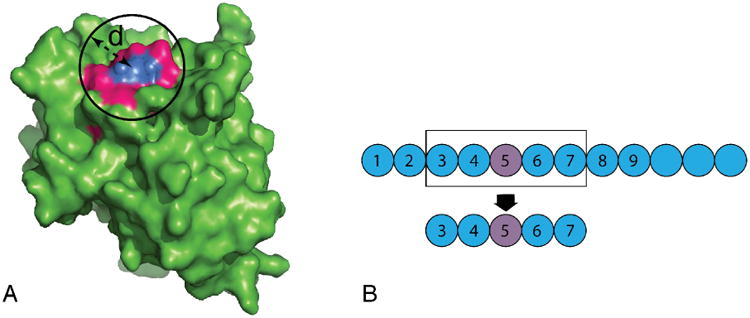
A) A surface patch defined by a target residue (blue) and its spatial neighboring residues (magenta) that fall within a virtual sphere of diameter, d, centered on the target residue. B) A sequence window centered on a target residue (purple).

Representative structure-based machine learning predictors include: SPPIDER (Porollo & Meller, 2007), PINUP (Liang, 2006), ProMate (Neuvirth, Raz, & Schreiber, 2004), and PIER (Kufareva, Budagyan, Raush, Totrov, & Abagyan, 2007) (for details see Table 1).

Structure-based methods offer several apparent advantages over sequence-based methods. For example, rather than making predictions for every residue in a protein, structure-based predictors need only to identify interfacial residues from among surface residues. However, structure-based prediction methods also have several disadvantages. First, their applicability is limited because they require knowledge of query protein structures, and the vast majority of proteins, especially those involved in transient binding interactions, do not have experimentally determined 3D structures. Transient interactions provide a mechanism for the cell to quickly respond to environmental stimuli, and are essential in the regulation of many disease-related pathways (Nooren & Thornton, 2003; Ozbabacan, Engin, Gursoy, & Keskin, 2011). Thus, reliable identification of interfaces involved in transient interactions has important implications in drug design. Second, structure-based methods are complicated by conformational changes that often occur when proteins interact with their binding partners (Zhou & Qin, 2007). Structure-based methods rely on structural features extracted from the query structure in its unbound state (or, for benchmarking cases, from a bound complex that has been separated into constituent proteins). Structural features extracted from unbound proteins may not exist in bound complexes due to conformational changes induced by or required for binding. Third, structure-based methods cannot handle disordered proteins. Higher organisms have a large number of intrinsically disordered proteins/regions (IDPs/IDRs), which become structured only upon binding to their partners (Dunker, Obradovic, Romero, Garner, & Brown, 2000). Such disordered regions - for which experimental structure information is, by definition, lacking - participate in many important cellular recognition events, and are believed to contribute to the ability of hub proteins to interact with multiple partners in protein-protein interaction networks (Dunker & Obradovic, 2001). Therefore, the development of sequence-based methods, which can reliably differentiate interfacial residues from non-interacting ones without requiring knowledge of protein structures, is of great interest.

Predicting protein interfaces from sequence alone is highly challenging and consequently sequence-based machine learning predictors are still underdeveloped. Given a protein sequence with L residues, a window of fixed width (typically 3-30 residues) is applied to the sequence, generating a total number of L overlapping windows, with each window centered on a target residue (Figure 1B). These sequence windows are used as input feature vectors, with sequences sometimes represented using physicochemical, statistical or predicted structural features, such as hydrophobicity or solvent accessibility. Representative sequence-based machine learning predictors include Yan et al.'s two-stage classifier (Yan, Dobbs, & Honavar, 2004), Sikic et al.'s random forest predictor (Šikić, Tomić, & Vlahoviček, 2009), PSIVER (Murakami & Mizuguchi, 2010), and the sequence-based version of PAIRpred (Afsar Minhas, Geiss, & Ben-Hur, 2013).

Currently most structure-based machine learning interface predictors have higher accuracy than sequence-based machine learning methods. One reason for this, mentioned above, is that most interfacial residues are on the protein surface, so structure-based methods can trivially identify surface residues and ignore all internal residues. Second, many protein-protein interfaces are highly segmented, comprising interfacial residues that are in close spatial proximity within the 3D structures, but far apart in the primary sequences of the proteins. The spatial positions of residues are key for macromolecular recognition. The absence of such information is therefore expected to reduce the performance of sequence-based predictors relative to structure-based ones. Third, geometric complementarity information is also readily available from 3D structures.

Meta-predictors

When individual predictors complement each other, a meta method, which pools the output of the individual methods to make a consensus prediction, often provides better performance than any of the member predictors. Therefore, the most reliable machine learning methods at present are meta-servers, such as meta-PPISP (Qin & Zhou, 2007) and CPORT (de Vries & Bonvin, 2011).

3 Basic Concepts and Evaluation

Existing machine learning interface predictors differ mainly in the specific type of machine learning classifier used and in the choice of features used as input to the classifier.

3.1 Characteristics of protein interfaces

To reliably predict interfacial residues, one needs to identify the characteristics that distinguish the interface region from the rest of the protein sequences or 3D structures. Such characteristics (or features) are critical for the success of a predictor. Widely used features in the literature include:

• Amino acid types. The most straightforward feature is an amino acid's identity or type. For classifiers that can process only numerical features, each type of commonly occurring amino acid can be represented as a binary vector of size 20 by 1. For example, alanine can be represented as [1,0,0,…,0].

• Physicochemical properties of amino acids. Commonly used physicochemical properties are hydrophobicity, charge and van der Waals volume. A database of numerical indices representing various physicochemical properties of amino acids and pairs of amino acids is provided in AAindex (Kawashima & Kanehisa, 2000).

• Interface propensity. The different physicochemical properties of amino acids result in differential interaction propensities. For example, in heterocomplexes, polar residues appear more frequently than do hydrophobic residues (Jones & Thornton, 1996) and aromatic amino acids tend to form stacking interactions. The higher its interface propensity, the more likely an amino acid is to appear in the interface as opposed to elsewhere on the protein surface. Such propensities are usually derived from an analysis of known structures in the PDB.

• Evolutionary information. Interfacial residues are important functional sites and tend to be conserved among homologs (Xue et al., 2011) or undergo correlated mutations (Hamer, Luo, Armitage, Reinert, & Deane, 2010). There are different ways to encode sequence conservation, and a widely used approach is to construct PSSMs (Position Specific Scoring Matrices) from multiple sequence alignments (MSAs). Each score in a PSSM is a log-likelihood ratio of an amino acid's appearance in a specific column of an MSA against a background distribution, representing the degree of conservation of the amino acid in that specific position; the higher the score, the higher the degree of conservation. Therefore, PSSMs capture important evolutionary information by exploiting the large number of available protein sequences, which are much easier to obtain than protein structures.

• Relative solvent accessibility. Most proteins recognize and interact with other proteins through their surface residues (i.e., residues with relatively high solvent accessible surface area) unless the interacting proteins undergo large conformational changes upon binding. Therefore, knowledge of protein surface residues can greatly reduce the prediction search space and increase prediction accuracy. Given the 3D structure of a protein, whether a residue is on the surface or not can be determined by calculating its relative accessible surface area (RASA) as follows:

  $$\mathit{\text{RASA}}=\frac{\mathit{\text{ASA}}\_\mathit{\text{residue}}\_\mathit{\text{in}}\_\mathit{\text{protein}}}{\mathit{\text{ASA}}\_\mathit{\text{free}}\_\mathit{\text{residue}}}$$

  where ASA_residue_in_protein is the surface area, i.e., accessible surface area (ASA), of the residue in the protein structure, and ASA_free_residue is the ASA of this residue in a “free” state. Surface areas of “free” residues are often estimated assuming that the residue X is the central residue in a tripeptide, G-X-G, or A-X-A, where G is Glycine and A is Alanine. A residue is generally regarded as a surface residue if its RASA is larger than 5% (Miller, Janin, Lesk, & Chothia, 1987; Porollo & Meller, 2007). Solvent accessibility of a residue in a protein can be calculated using software, for example, STRIDE (Frishman & Argos, 1995; Heinig & Frishman, 2004).

  When the protein structure is not available (which is the case for most proteins), one has to rely on bioinformatics methods to predict solvent accessibilities.

• Surface shape. The shape of a protein surface is also a useful indicator of interacting sites. One widely used measure for the concavity or convexity of the neighborhood of an atom in a protein is the CX value (Pintar, Carugo, & Pongor, 2002). To calculate the CX value of an atom, a sphere is centered on the target atom, and CX = Vext / Vint, where Vint is the volume occupied by the protein, and Vext is the free volume in the sphere.

Because a single feature cannot reliably discriminate interfacial residues from the rest of the residues in a protein, most existing prediction methods use a combination of several features. The most valuable feature identified so far is the evolutionary information encoded in PSSMs (refer to (Yan & Wang, 2014) for details regarding the relative contributions of individual features in predicting DNA-binding sites in proteins).

3.2 Interface definitions

There are several ways to define an interface. It is important to use the same interface definition when comparing different prediction methods. Commonly used definitions in the literature include:

• Heavy atom distance: A residue is an interfacial residue if any heavy atom (non-hydrogen atom) of the residue is within D_thr angstroms of any heavy atom of a residue in the interacting protein chain, where D_thr is the threshold diameter and usually ranges from 4-6 Å (Afsar Minhas et al., 2013; Xue et al., 2011). This is probably the most commonly used definition.

• CA-CA distance: Two residues in different chains interact if their CA atoms are within D_thr Ångstroms. A reasonable value for D_thr is 8 Å.

• van der Waals surface distance: Two residues in different chains interact if their van der Waals surfaces are within D_thr Å. D_thr is usually set around 0.5 Å (Jordan et al., 2012).

• ΔASA (Delta Accessible Surface Area): A residue is an interfacial residue if the change in its ASA upon complexation (going from a monomeric state to a dimeric state) is larger than 1 Ų (Jones & M, 1997).

i-RMSDs (interface root-mean-squared-deviation) and Fnat (fraction of native residue-residue contacts) are also widely used to evaluate the models generated by docking programs as used in the international blind experiment – CAPRI (Critical Assessment of Predicted Interactions) (Lensink & Wodak, 2013). To calculate i-RMSDs, the backbone atoms of interface residues within 10Å from the partner molecules of the reference complex are superimposed upon their equivalents of a docked model and the corresponding RMSD is calculated. (Méndez, Leplae, De Maria, & Wodak, 2003).

Fnat is defined as the number of correctly predicted residue-residue contacts in a docked model divided by the total number of contacts in the target complex using a 5Å distance cut-off (CAPRI definition).

3.3 Benchmark Datasets and Dealing with Unbalanced Data

The PDB (Protein Data Bank, www.rcsb.org) (Berman et al., 2000) is the largest database of high-resolution 3D structures, including both monomeric protein structures and structures of proteins in complexes with other molecules, including other proteins, DNAs, RNAs and cofactors or other small molecules. High quality protein-protein complexes (with a resolution less than 3 to 3.5 Å) can be extracted from the PDB to serve as training and testing datasets for interface predictors.

In globular proteins, the percentage of all residues that lie in the interface typically ranges from 10% to 18%, varying across different types of protein-protein interactions (Xue et al., 2011). In addition to the complex nature of physicochemical recognition, the highly unbalanced nature of the data (i.e., the number of non-interfacial residues is much larger than the number of interfacial residues) imposes a further challenge on the design of reliable interface predictors. When trained with highly unbalanced data, machine learning classifiers tend to over-predict the over-represented class. To avoid skewed performance of a predictor on unbalanced data, a widely used practice is to under-sample the negative data (i.e., non-interfacial residues) several times and to train an ensemble of classifiers using these sampled balanced datasets (i.e., equal number of interface instances and non-interface instances) (Ahmad & Mizuguchi, 2011). Another strategy is to set a larger penalty for misclassification of interfacial residues directly in the machine learning algorithm, for example, by adjusting the C parameter of an SVM. To objectively evaluate the performance of predictors, the testing dataset must be non-redundant, but should not be balanced, i.e., it should reflect the natural distribution of positive and negative examples. For constructing non-redundant datasets, a 30% sequence identity cutoff is commonly used.

Although the protein-protein docking benchmark 4.0 (DB4) (Hwang, Vreven, Janin, & Weng, 2010) was originally designed to evaluate docking programs, it also can serve as a good benchmark test dataset for evaluating protein-protein interface predictors. The DB4 dataset consists of 176 non-redundant protein-protein complexes and their corresponding component protein structures in the unbound state. The selected complexes represent three types of protein-protein interactions (enzyme-inhibitor, antigen-antibody, and others) and are grouped into 3 classes based on the degree of conformational changes upon binding (which is correlated with the expected “difficulty” for docking). The DB4 dataset is thus especially well suited for testing the robustness of structure-based interface predictors in dealing with conformational changes upon binding.

PIFACE -- a non-redundant database of protein-protein interface structures extracted from the PDB (Cukuroglu, Gursoy, Nussinov, & Keskin, 2014) also provides good source of training data for positive cases (i.e., interfaces).

3.4 Evaluation

3.4.1 Evaluation metrics

Predicting interfacial residues is usually formulated as a two-class classification problem, where interfacial residues belong to the positive class and non-interfacial residues to the negative class. To evaluate the performance of computational methods in predicting the interfacial residues of test proteins, several standard performance measures are used. These include: Sensitivity (Recall), Specificity (Precision), F1 measure, Matthew's correlation coefficient (MCC), and Accuracy (Baldi, Brunak, Chauvin, Andersen, & Nielsen, 2000), defined as follows:

$$\mathit{\text{Sensitivity}}(\mathit{\text{recall}})=\mathit{\text{TP}}/(\mathit{\text{TP}}+\mathit{\text{FN}})$$

$$\mathit{\text{Specificity}}(\mathit{\text{precision}})=\mathit{\text{TP}}/(\mathit{\text{TP}}+\mathit{\text{FP}})$$

$$F1=2\times \mathit{\text{precision}}\times \mathit{\text{recall}}/(\mathit{\text{precision}}+\mathit{\text{recall}})$$

$$\mathit{\text{MCC}}=\frac{\mathit{\text{TP}}\times \mathit{\text{TN}}-\mathit{\text{FP}}\times \mathit{\text{FN}}}{\sqrt{(\mathit{\text{TP}}+\mathit{\text{FN}})(\mathit{\text{TP}}+\mathit{\text{FP}})(\mathit{\text{TN}}+\mathit{\text{FP}})(\mathit{\text{TN}}+\mathit{\text{FN}})}}$$

$$\mathit{\text{Accuracy}}=\mathit{\text{TP}}/(\mathit{\text{TP}}+\mathit{\text{TN}}+\mathit{\text{FP}}+\mathit{\text{FN}})(\text{widely used but not recommended})$$

where TP (True Positive) is defined as the number of interface residues that are correctly predicted to be interface residues; FP (False Positive) is the number of residues that are incorrectly predicted to be interface residues; TN (True Negative) is the number of residues that are correctly predicted to be non-interface residues); and FN (False Negative) is the number of residues that are incorrectly predicted to be non-interface residues.

Sensitivity measures the proportion of actual interfacial residues that are correctly predicted as interfacial, while Specificity measures the proportion of predicted interfacial residues that are actual interfacial residues. (Note that in medical statistics literature a different definition of Specificity is often used, where Specificity is defined as the proportion of negative instances that are correctly identified as such, i.e., “Sensitivity” for the negative class (Baldi et al., 2000). F1 is the harmonic mean of sensitivity and specificity. We can also treat the binary prediction and the actual interface as two random variables taking only the values of 1 and 0, where 1 indicates a predicted or actual interfacial residue, and 0 indicates a predicted or actual non-interfacial residue. Then we can use MCC to measure the correlation coefficient between the prediction and the actual interface random variables.

Note that when the data are highly unbalanced (as they usually are in the interface prediction problem), accuracy is not an appropriate performance evaluation measure. For example, when only 10% of the test residues are actual interfacial residues, a “dumb” predictor that simply predicts all residues as non-interfacial residues will obtain an accuracy of 90%.

An advantage of predictors trained using machine learning is that it is possible to trade off one performance measure against another by varying the prediction score cutoff. For example, in some situations, experimental scientists may wish to obtain only a small number of interfacial residues predicted with a high degree of confidence. In this case, it makes sense to choose a relatively high score cutoff, which will return predictions with high specificity but low sensitivity (i.e., some actual interfacial residues will be predicted as non-interfacial). In contrast, choosing a low score cutoff can provide better coverage of actual interfacial residues, but at the risk of a higher false positive rate. Hence, reporting the performance of a predictor against all possible score cutoffs provides a much more complete and rigorous evaluation of its performance. Specificity vs. Sensitivity plots (also called Precision-Recall plots) or the ROC curve (true positive rate vs. false positive rate) show the trade-off between two performance measures, and allow experimentalists to choose a cutoff that fits their specific requirements for prediction accuracy. Such plots also provide a clear visualization of the comparative performance of different classifiers. For example, it is easy to tell whether two predictors have complementary prediction power, which is indicated by crossing curves for the two predictors. This allows users to combine the output from two complementary predictors into one combined score to gain a better performance.

3.4.2 Statistical comparison of two or more predictors

Cross-validation (CV) and leave-one-out are widely used in the field of machine learning to evaluate the performance of classifiers. N-fold cross-validation equally divides the dataset into N parts, trains the classifier on N – 1 parts and evaluates the trained classifier on the left-out part. The same procedure is repeated by leaving each of the N parts out as test data, and a total of N performance measures are obtained. When comparing two predictors, a pairwise t-test is often used to test the null hypothesis that the two predictors have the same mean performance (estimated using cross-validation), i.e., the differences between them are no greater than what would be expected at random. As Demšar (Demšar, 2006)) points out, since these samples are usually related, a lot of care is needed in designing the statistical procedures and tests that avoid problems with biased estimations of variance. Dietterich (Dietterich, 1998) recommends 5×2cv t-test that overcomes the problem of underestimated variance and the consequently elevated Type I error of the more traditional paired t-test over folds of the usual k -fold cross validation.

Salzberg (Salzberg, 1997) points out that in comparing two predictors using cross-validation, the common practice of using a paired t-test to test the null hypothesis that the two predictors have the same mean performance is problematic when the test sets are not independent. In such cases, Salzberg (Salzberg, 1997) recommends a simple way to compare the two predictors is to compare the percentage of times A got right that B got wrong with the percentage of times B got right that A got wrong, and throw out the ties. One can then use a simple binomial test for the comparison, with the Bonferroni adjustment for multiple tests. Note, however, that the binomial test is a relatively weak test that does not handle quantitative differences between predictors, or consider the frequency of agreement between two predictors. Nor can it be used to compare multiple predictors. Demšar (Demšar, 2006)) recommends a non-parametric pairwise statistical test, such as Wilcoxon signed-rank test for comparing two predictors; and analysis of variance (ANOVA) followed by Tukey test or the non-parametric Friedman test or the Nemenyi test in the case of multiple predictors (for more details, refer to the excellent review by Demšar (Demšar, 2006)).

3.4.3 Statistical comparison with random predictions

Any reasonable interface predictor should at least outperform random predictions. Random predictions can be formulated by the hypergeometric distribution: X∼HG (N, M, K), where X is the number of actual interfacial residues in the top K predictions, N is the total number of instances (i.e., total number of residues in query proteins), and M is the total number of actual interfacial residues. $P(X=x)=\left(\begin{array}{c}M\\ x\end{array}\right)\left(\begin{array}{c}N-M\\ K-x\end{array}\right)/\left(\begin{array}{c}N\\ K\end{array}\right)$ is the probability that there are x actual interfacial residues in the top K randomly predicted interfacial residues.

3.5 An important caveat in evaluation

A critical mistake in performance evaluation, which still repeatedly appears in the recent published literature, should be noted by predictor developers and reviewers. This caveat regards the use of CV or leave-one-out procedures to evaluate protein interface predictions. Most, if not all, machine learning-based interface predictors use sliding windows or surface patches to generate the training and testing instances. Individual instances (i.e., sequence windows or surface patches of amino acids) obtained from the same protein have large overlaps with their neighboring instances; thus, they are not independent from each other. To objectively evaluate the performance of an interface predictor, one should perform CV or leave-one-out on the protein level (or protein complex level) instead of on the instance (i.e., a window or a surface patch of amino acids) level, because users naturally want to know the prediction accuracy on individual input protein(s) instead of a bag of mixed residues from multiple proteins. Using CV on the instance level can yield overly optimistic measures of performance. Walia et al. (Walia et al., 2012) systematically compared sequence-based and structure-based methods with different features and different machine learning classifiers on different datasets, using leave-one-out over instances vs. leave-one-out over proteins. In all cases, evaluation using leave-one-out over instances gave a misleadingly higher estimate of the prediction performance compared with the estimates by leave-one-out over proteins (Table 2).

Table 2. The comparison of instance-based evaluation and protein-based evaluation in terms of AUC.

Cross-validation (CV) over instances yields overly optimistic measures of performance, while CV over proteins gives a more realistic estimation for practical applications. Three different classifiers are evaluated: Naïve Bayes (NB), Support Vector Machine (SVM) with linear kernel (LK), and SVM with radial basis function (RBF) kernel. Three types of sequence-derived features are used: IDseq (amino acid identity), PSSM, and smoothed PSSM (Smo PSSM). Only sequence-based predictors are listed here, but structure-based predictors support the same conclusion; see (Walia et al., 2012) for details. Table is reproduced with the permission of Walia et al. (Walia et al., 2012).

Feature	IDSeq	IDSeq	IDSeq	PSSM	PSSM	PSSM	Smo PSSM	Smo PSSM	Smo PSSM
Classifier	NB	LK	RBFK	NB	LK	RBFK	NB	LK	RBFK
Instance-based	0.73	0.72	0.73	0.74	0.78	0.80	0.75	0.77	0.78
Protein-based	0.68	0.67	0.68	0.71	0.72	0.74	0.68	0.70	0.72

4. Partners Do Matter

Despite considerable efforts dedicated to the development of sophisticated data-driven protein-protein interface predictors, most have so far ignored the fact that many proteins use different interacting surfaces to interact with different binding partners (partner-specificity). As mentioned earlier, partner-specificity is especially important in transient interactions such as those that occur in signal transduction pathways (Xue et al., 2011). The high degree of partner-specificity in transient interactions makes them especially appealing as potential targets for selective therapeutic inhibitors (Rudolph, 2007). Available non-partner-specific (NPS) prediction methods (i.e., those that do not take into consideration a protein's binding partner) have lower reliability in predicting transient binding sites compared with their performance on obligate interfaces (de Vries & Bonvin, 2008; Panchenko, Kondrashov, & Bryant, 2004). Hence, reliable methods for predicting interfaces in transient protein-protein interactions are needed.

Only within the last 5 years has the importance of partner-specificity for reliably predicting interfaces been fully realized. The first partner-specific method for predicting interfaces between two protein domains was i-Patch (Hamer et al., 2010). I-Patch requires as input two MSAs for the two query domains, and each row of the two MSAs must be concatenated in such that interacting homologs are concatenated into a single one row (this requirement imposes a limitation on the application of this method). The term “partner-specific interface prediction” was first used by our group in a paper published in 2011 (Xue et al., 2011). In that study, we conducted a systematic analysis of partner-specific interface conservation and demonstrated, for the first time, that interface locations are, in fact, highly conserved in transient protein-protein interactions, despite previous reports to the contrary (Grishin & Phillips, 1994), as discussed earlier. We implemented the first partner-specific protein-protein interface predictor, PS-HomPPI, and showed that it was more reliable than its non-partner-specific counterpart, NPS-HomPPI. Subsequently, two machine learning-based partner-specific interface prediction approaches were published: PPiPP (Ahmad & Mizuguchi, 2011), which is an ensemble of NN (Neural Network) based methods, and PAIRpred (Afsar Minhas et al., 2013), which is a pairwise kernel based SVM (Support Vector Machines) method. PPiPP is a sequence-based method, which uses a binary encoding of amino acids and PSSMs as features. It uses an ensemble of 24 NNs trained on datasets generated from different window sizes and different samples of negative data; the average of the 24 NNs prediction scores is the final score (Ahmad & Mizuguchi, 2011). PAIRpred has both a sequence-based and a structure-based version (Afsar Minhas et al., 2013). To predict whether two residues interact with each other, both PPiPP and PAIRpred use features of the query residue pair and their neighboring residues as input. Both methods have been shown to outperform several state-of-the-art non-partner-specific (NPS) methods (Afsar Minhas et al., 2013; Ahmad & Mizuguchi, 2011) (Figure 2).

Figure 2. Partner-specific interface predictors outperform non-partner-specific predictors.

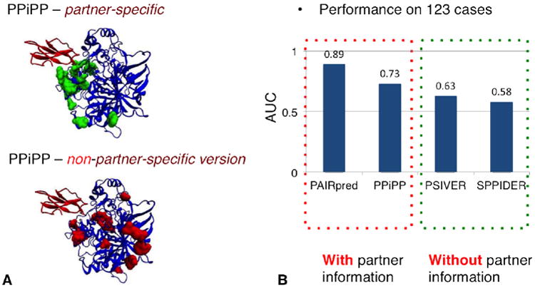
(A) A comparison of the top 20 predicted interfacial residues for a complex of Acetylcholinesterase (blue ribbons) and Toxin F-VII Fasciculin-2 (red ribbons) (PDB ID: 1MAH) by the partner-specific method, PPIPP (Ahmad & Mizuguchi, 2011), and the corresponding non-partner-specific version. By including partner information, PPIPP is able to predict interfacial residues (green) clustering around the interaction location specific to the binding partner whereas those predicted by the non-partner-specific method (red) are scattered over the surface of query protein. Figure credit: (Ahmad & Mizuguchi, 2011)(B) Prediction performance comparisons over a set of 123 non-redundant protein-protein complexes in Docking Benchmark 3.0 (Hwang, Pierce, Mintseris, Janin, & Weng, 2008). We compared two partner-specific predictors, PAIRpred (Afsar Minhas et al., 2013) and PPiPP (a sequence-based predictor) (Ahmad & Mizuguchi, 2011), with two non-partner-specific machine learning predictors: PSIVER, a sequence-based predictor (Murakami & Mizuguchi, 2010) and SPPIDER, a structure-based predictor (Porollo & Meller, 2007). With partner information, PAIRpred and PPiPP outperform the two predictors that do not consider partner information when making predictions, improving Area Under Curves (AUCs) from 0.63 (PSIVER) and 0.58 (SPPIDER) to 0.73 (PPiPP) and 0.89 (PAIRpred). AUC values are extracted from (Afsar Minhas et al., 2013; Ahmad & Mizuguchi, 2011).

Partner-specific interface prediction is an important advance in protein-protein interface prediction. By exploiting binding partner information, partner-specific interface predictors generally out-perform their non-partner-specific counterparts (Afsar Minhas et al., 2013; Ahmad & Mizuguchi, 2011; Xue et al., 2011). Improved partner-specific interface predictors will likely be the focus in designing the next generation of interface predictors.

5 Interface Prediction can Enhance Computational Docking

Another major and drastically different strategy for predicting protein-protein interfaces is protein-protein docking. Computational docking methods are valuable tools for predicting the 3D structures of protein complexes, from which the interfacial residues can be extracted. Docking approaches aim to generate structures with low interaction energies by sampling a very large number of possible interaction modes (the sampling step) and evaluating each conformation using energy functions (the scoring step) (Figure 3).

Figure 3. Protein-protein docking and its two major challenges.

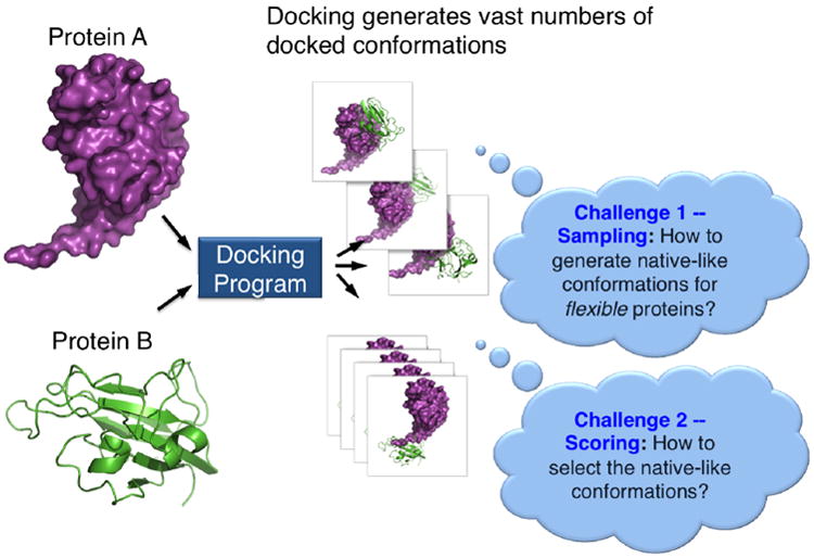
Despite recent advances displayed in the international community docking competition – CAPRI (Lensink & Wodak, 2013), docking still faces two major technical challenges that limit its reliability and hinder its large-scale application to complete proteomes. The first challenge is in the sampling step, especially in cases where conformational changes take place upon binding (Alexandre Bonvin, 2006; Zacharias, 2010). The flexibility of protein molecules generates a vast number of possible conformations that must be sampled and evaluated. The second challenge lies in the scoring step. Our understanding of the energetic aspects of protein interactions is still incomplete and current scoring functions have limited ability to single out native-like conformations from the vast number of possible docked conformations (Kastritis & Bonvin, 2010; Lensink & Wodak, 2013)

Docking and machine learning-based interface predictions both have strengths and weaknesses, and they complement each other. Docking, by nature, is a partner-specific method. Because docking is based on geometric and energetic models, in theory, it does not require a large amount of pre-existing data as a training set. Machine learning methods can seamlessly integrate heterogeneous sources of existing experimental data and extract interaction rules in order to make interface predictions. For example, machine learning methods can make use of evolution information extracted from MSAs, which provides critical complementary information to docking. In addition, machine learning predictors are typically much faster and require fewer computational resources than docking. To process one query, a machine learning predictor requires a few seconds to 1 hour, compared with minutes to several hours or days on a single processor for docking programs. Although machine learning predictors tend to predict at the residue level and can have a high false positive rate, they can be used to conduct a fast pre-screen to identify several potential binding patches that can be further tested and refined by high-resolution (i.e., at the atomic level) docking. Recently, binding patches predicted by machine learning have been shown to efficiently narrow down the search space for docking (see below).

Guided docking, in which experimentally determined interfacial contacts are used to constrain the docking search space, has been highly successful. The pioneering method, HADDOCK (High Ambiguity Driven protein–protein Docking) (de Vries, van Dijk, & Bonvin, 2010b; Dominguez et al., 2003), can use experimentally determined interface data (e.g., from chemical shift perturbation or mutagenesis experiments) as distance restraints in its sampling process. It can generate near-native conformations for cases that undergo medium to large conformational changes upon binding (Karaca & Bonvin, 2011). The use of experimental restraints allows HADDOCK to concentrate its search around relevant regions of the interaction space and refine the solutions allowing for explicit flexibility.

The HADDOCK group has also explored the use of predicted interfacial residues as docking restraints, and obtained improved results compared with the ab initio version of HADDOCK and competitive results compared with a state-of-the-art ab initio docking method, ZDOCK (de Vries & Bonvin, 2011). These results are encouraging because interface prediction-guided docking has the promise of effectively narrowing down the sampling space of docking, thus reducing the computational cost. Currently, interface prediction-guided docking defines a lower bound for data-driven docking. With future improvements, interface predictions should further enhance the reliability of the 3D protein complex models by computational docking.

Homology-based interface predictions have also been used to improve the scoring of docked models. Li and Kihara (Li & Kihara, 2012) concluded that (non-partner-specific) machine learning-based predicted interfaces cannot be used to reliably identify near-native conformations. Subsequently, however, our group demonstrated that DockRank, a method that uses partner-specific homology-based interface predictions, can significantly improve the scoring of docked poses (Xue, Jordan, Yasser, Dobbs, & Honavar, 2014). DockRank outperforms several energy-based scoring functions and three non-partner-specific machine learning and homology-based methods.

Conversely, docking can also facilitate interface predictions: In the context of the CAPRI experiment, it has been shown that generated docking decoys can assist interface predictions even when considering cases where no near-native solutions could be generated (de Vries et al., 2010a). Similar observations have been made by the ZDOCK group (Hwang, Vreven, & Weng, 2014).

6 Challenges and Future Directions

Protein interface prediction will continue to be a highly challenging and important research topic. Reliable identification of protein binding sites has wide applications in computational protein design and rational drug design. In the past 20 years, there has been significant progress in computational prediction of protein interfaces, but there is still much room for improving the reliability of interface predictors.

To further improve interface prediction, improved feature extraction methods and feature representations that can effectively capture the complexities of protein recognition in diverse types of interactions will be important. For example, we now know that transient and obligate interactions have different recognition patterns and should be treated separately. Also, even though most existing machine learning interface predictors are structure-based, typically the only structural information used to encode input feature vectors is statistical information about surface patches; information about the spatial arrangement of residues and/or atoms has been largely ignored. Most importantly, the evidence is now clear that consideration of specific binding partners is essential for reliably predicting binding sites. Both the feature representation and the design of the classifiers must take into account the partner-specific nature of transient protein interactions.

The availability of high throughput data regarding protein-protein interaction partners also may provide valuable co-evolutionary information for predicting partner-specific protein-protein interfaces. Recently, inverse-covariance-matrix based methods have brought breakthrough advances in protein structure prediction (reviewed in (Marks et al., 2012)). With unprecedented accuracy, this type of statistical model predicts amino acid contact pairs that are in close spatial proximity within a 3D structure by calculating the correlation between two columns, conditional on the rest of columns in an MSA; then the predicted contacts are used as distance restraints to fold proteins with impressive accuracy. Contacting pairs of amino acids in protein-protein interfaces are also expected to undergo correlated mutations (Hamer et al., 2010; Lunt et al., 2010). In fact, inverse-covariance-matrix based methods have already been successfully applied to predict interfaces of query protein pairs (Halabi et al., 2009; Hopf et al., 2014; Lunt et al., 2010). However, the applicability of this method to large-scale protein interface predictions is limited by the fact that it requires knowledge of whether two homologs of the query proteins interact with each other. With massive-throughput sequencing capabilities and high-throughput techniques for determining protein-protein interactions (such as yeast 2-hybrid assays and chip-based assays) or advances in computational prediction of protein-protein interaction partners (for example, (Kotlyar et al., 2015)), this limitation will eventually be addressed, making this solution applicable on a larger scale.

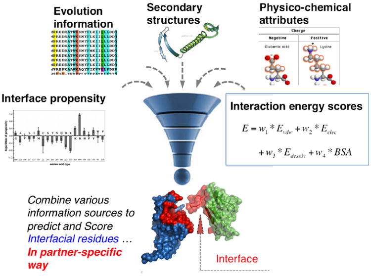
Finally, another promising future direction is developing effective ways to combine energy model-driven docking with data-driven interface prediction methods. The PDB has been accumulating a large number of atomic resolution structures of protein-protein complexes: 104,570 as of Oct. 1st, 2015¹. This large amount of high-resolution structure data, together with the enormous number of protein sequences now available, provide rich training data for machine learning algorithms to learn statistical interaction patterns. Combining low-resolution statistical interaction patterns learned from experimental data with high-resolution computational docking has the potential to dramatically improve interface predictions -- and reveal both structural and functional information about protein-protein interactions (Figure 4).

Figure 4. Machine learning toward improved 3D protein interaction prediction.

References

- Afsar Minhas FUA, Geiss BJ, Ben-Hur A. PAIRpred: Partner-specific prediction of interacting residues from sequence and structure. Proteins: Structure, Function, and Bioinformatics. 2013;82(7):1142–1155. doi: 10.1002/prot.24479. http://doi.org/10.1002/prot.24479. [DOI] [PMC free article] [PubMed] [Google Scholar]
- Ahmad S, Mizuguchi K. Partner-Aware Prediction of Interacting Residues in Protein-Protein Complexes from Sequence Data. PLoS One. 2011;6(12):e29104. doi: 10.1371/journal.pone.0029104. http://doi.org/10.1371/journal.pone.0029104. [DOI] [PMC free article] [PubMed] [Google Scholar]
- Baldi P, Brunak S, Chauvin Y, Andersen CA, Nielsen H. Assessing the accuracy of prediction algorithms for classification: an overview. Bioinformatics. 2000;16(5):412–424. doi: 10.1093/bioinformatics/16.5.412. [DOI] [PubMed] [Google Scholar]
- Berman HM, Westbrook J, Feng Z, Gilliland G, Bhat TN, Weissig H, et al. The Protein Data Bank. Nucleic Acids Research. 2000;28(1):235–242. doi: 10.1093/nar/28.1.235. http://doi.org/10.1093/nar/28.1.235. [DOI] [PMC free article] [PubMed] [Google Scholar]
- Bonvin Alexandre. Flexible protein-protein docking. Current Opinion in Structural Biology. 2006;16(2):194–200. doi: 10.1016/j.sbi.2006.02.002. http://doi.org/10.1016/j.sbi.2006.02.002. [DOI] [PubMed] [Google Scholar]
- Caffrey DR, Somaroo S, Hughes JD, Mintseris J, Huang ES. Are protein–protein interfaces more conserved in sequence than the rest of the protein surface? Protein Science. 2004;13(1):190–202. doi: 10.1110/ps.03323604. http://doi.org/10.1110/ps.03323604. [DOI] [PMC free article] [PubMed] [Google Scholar]
- Chen H, Zhou HX. Prediction of interface residues in protein-protein complexes by a consensus neural network method: test against NMR data. Proteins: Structure, Function, and Bioinformatics. 2005;61(1):21–35. doi: 10.1002/prot.20514. http://doi.org/10.1002/prot.20514. [DOI] [PubMed] [Google Scholar]
- Cukuroglu E, Gursoy A, Nussinov R, Keskin O. Non-redundant unique interface structures as templates for modeling protein interactions. PLoS One. 2014;9(1):e86738. doi: 10.1371/journal.pone.0086738. http://doi.org/10.1371/journal.pone.0086738. [DOI] [PMC free article] [PubMed] [Google Scholar]
- de Vries SJ, Bonvin A. How proteins get in touch: interface prediction in the study of biomolecular complexes. Current Protein and Peptide Science. 2008 doi: 10.2174/138920308785132712. [DOI] [PubMed] [Google Scholar]
- de Vries SJ, Bonvin A. CPORT: A Consensus Interface Predictor and Its Performance in Prediction-Driven Docking with HADDOCK. PLoS One. 2011;6(3):e17695. doi: 10.1371/journal.pone.0017695. http://doi.org/10.1371/journal.pone.0017695. [DOI] [PMC free article] [PubMed] [Google Scholar]
- de Vries SJ, Melquiond ASJ, Kastritis PL, Karaca E, Bordogna A, van Dijk M, et al. Strengths and weaknesses of data-driven docking in critical assessment of prediction of interactions. Proteins: Structure, Function, and Bioinformatics. 2010a;78(15):3242–3249. doi: 10.1002/prot.22814. http://doi.org/10.1002/prot.22814. [DOI] [PubMed] [Google Scholar]
- de Vries SJ, van Dijk ADJ, Bonvin A. WHISCY: What information does surface conservation yield? Application to data-driven docking. Proteins: Structure, Function, and Bioinformatics. 2006;63(3):479–489. doi: 10.1002/prot.20842. http://doi.org/10.1002/prot.20842. [DOI] [PubMed] [Google Scholar]
- de Vries SJ, van Dijk M, Bonvin A. The HADDOCK web server for data-driven biomolecular docking. Nature Protocols. 2010b;5(5):883–897. doi: 10.1038/nprot.2010.32. http://doi.org/10.1038/nprot.2010.32. [DOI] [PubMed] [Google Scholar]
- Demšar J. Statistical Comparisons of Classifiers over Multiple Data Sets. The Journal of Machine Learning Research. 2006;7:1–30. [Google Scholar]
- Dietterich TG. Approximate Statistical Tests for Comparing Supervised Classification Learning Algorithms. Dx Doi org. 1998;10(7):1895–1923. doi: 10.1162/089976698300017197. http://doi.org/10.1162/089976698300017197. [DOI] [PubMed] [Google Scholar]
- Dominguez C, Boelens R, Bonvin A. HADDOCK: a protein-protein docking approach based on biochemical or biophysical information. Journal of the American Chemical Society. 2003;125(7):1731–1737. doi: 10.1021/ja026939x. http://doi.org/10.1021/ja026939x. [DOI] [PubMed] [Google Scholar]
- Dunker AK, Obradovic Z. The protein trinity--linking function and disorder. Nature Biotechnology. 2001;19(9):805–806. doi: 10.1038/nbt0901-805. http://doi.org/10.1038/nbt0901-805. [DOI] [PubMed] [Google Scholar]
- Dunker AK, Obradovic Z, Romero P, Garner EC, Brown CJ. Intrinsic protein disorder in complete genomes. Genome Informatics Workshop on Genome Informatics. 2000;11:161–171. [PubMed] [Google Scholar]
- Esmaielbeiki R, Krawczyk K, Knapp B, Nebel JC, Deane CM. Progress and challenges in predicting protein interfaces. Briefings in Bioinformatics. 2015:bbv027. doi: 10.1093/bib/bbv027. http://doi.org/10.1093/bib/bbv027. [DOI] [PMC free article] [PubMed]
- Ezkurdia I, Bartoli L, Fariselli P, Casadio R, Valencia A, Tress ML. Progress and challenges in predicting protein–protein interaction sites. Briefings in Bioinformatics. 2009;10(3):bbp021–246. doi: 10.1093/bib/bbp021. http://doi.org/10.1093/bib/bbp021. [DOI] [PubMed] [Google Scholar]
- Frishman D, Argos P. Knowledge-based protein secondary structure assignment. Proteins. 1995;23(4):566–579. doi: 10.1002/prot.340230412. http://doi.org/10.1002/prot.340230412. [DOI] [PubMed] [Google Scholar]
- Göbl C, Madl T, Simon B, Sattler M. NMR approaches for structural analysis of multidomain proteins and complexes in solution. Progress in Nuclear Magnetic Resonance Spectroscopy. 2014;80:26–63. doi: 10.1016/j.pnmrs.2014.05.003. http://doi.org/10.1016/j.pnmrs.2014.05.003. [DOI] [PubMed] [Google Scholar]
- Grishin NV, Phillips MA. The subunit interfaces of oligomeric enzymes are conserved to a similar extent to the overall protein sequences. Protein Science : a Publication of the Protein Society. 1994;3(12):2455–2458. doi: 10.1002/pro.5560031231. http://doi.org/10.1002/pro.5560031231. [DOI] [PMC free article] [PubMed] [Google Scholar]
- Halabi N, Rivoire O, Leibler S, Ranganathan R. Protein sectors: evolutionary units of three-dimensional structure. Cell. 2009;138(4):774–786. doi: 10.1016/j.cell.2009.07.038. http://doi.org/10.1016/j.cell.2009.07.038. [DOI] [PMC free article] [PubMed] [Google Scholar]
- Hamer R, Luo Q, Armitage JP, Reinert G, Deane CM. i-Patch: Interprotein contact prediction using local network information. Proteins: Structure, Function, and Bioinformatics. 2010;78(13):2781–2797. doi: 10.1002/prot.22792. http://doi.org/10.1002/prot.22792. [DOI] [PubMed] [Google Scholar]
- Heinig M, Frishman D. STRIDE: a web server for secondary structure assignment from known atomic coordinates of proteins. Nucleic Acids Research. 2004;32(Web Server issue):W500–2. doi: 10.1093/nar/gkh429. http://doi.org/10.1093/nar/gkh429. [DOI] [PMC free article] [PubMed] [Google Scholar]
- Hoofnagle AN, Resing KA, Ahn NG. Protein analysis by hydrogen exchange mass spectrometry. Annual Review of Biophysics and Biomolecular Structure. 2003;32(1):1–25. doi: 10.1146/annurev.biophys.32.110601.142417. http://doi.org/10.1146/annurev.biophys.32.110601.142417. [DOI] [PubMed] [Google Scholar]
- Hopf TA, Schärfe CPI, Rodrigues JPGLM, Green AG, Kohlbacher O, Sander C, et al. Sequence co-evolution gives 3D contacts and structures of protein complexes. eLife. 2014;3 doi: 10.7554/eLife.03430. http://doi.org/10.7554/eLife.03430. [DOI] [PMC free article] [PubMed] [Google Scholar]
- Hwang H, Vreven T, Weng Z. Binding interface prediction by combining protein-protein docking results. Proteins: Structure, Function, and Bioinformatics. 2014;82(1):57–66. doi: 10.1002/prot.24354. http://doi.org/10.1002/prot.24354. [DOI] [PMC free article] [PubMed] [Google Scholar]
- Hwang H, Vreven T, Janin J, Weng Z. Protein–protein docking benchmark version 4.0. Proteins: Structure, Function, and Bioinformatics. 2010;78(15):3111–3114. doi: 10.1002/prot.22830. http://doi.org/10.1002/prot.22830. [DOI] [PMC free article] [PubMed] [Google Scholar]
- Jones S, M TJ. Analysis of Protein-Protein Interaction Sites using Surface Patches. 1997:1–12. doi: 10.1006/jmbi.1997.1234. [DOI] [PubMed] [Google Scholar]
- Jones S, Thornton JM. Principles of protein-protein interactions. Proceedings of the National Academy of Sciences. 1996;93(1):13–20. doi: 10.1073/pnas.93.1.13. [DOI] [PMC free article] [PubMed] [Google Scholar]
- Jordan RA, EL-Manzalawy Y, Dobbs D, Honavar V. Predicting protein-protein interface residues using local surface structural similarity. BMC Bioinformatics. 2012;13(1):41. doi: 10.1186/1471-2105-13-41. http://doi.org/10.1186/1471-2105-13-41. [DOI] [PMC free article] [PubMed] [Google Scholar]
- Jubb H, Blundell TL, Ascher DB. Flexibility and small pockets at protein-protein interfaces: New insights into druggability. Progress in Biophysics and Molecular Biology. 2015 doi: 10.1016/j.pbiomolbio.2015.01.009. http://doi.org/10.1016/j.pbiomolbio.2015.01.009. [DOI] [PMC free article] [PubMed]
- Karaca E, Bonvin A. A multidomain flexible docking approach to deal with large conformational changes in the modeling of biomolecular complexes. Structure (London, England : 1993) 2011;19(4):555–565. doi: 10.1016/j.str.2011.01.014. http://doi.org/10.1016/j.str.2011.01.014. [DOI] [PubMed] [Google Scholar]
- Kastritis PL, Bonvin A. Are scoring functions in protein-protein docking ready to predict interactomes? Clues from a novel binding affinity benchmark. Journal of Proteome Research. 2010;9(5):2216–2225. doi: 10.1021/pr9009854. http://doi.org/10.1021/pr9009854. [DOI] [PubMed] [Google Scholar]
- Kaveti S, Engen JR. Protein interactions probed with mass spectrometry. Methods in Molecular Biology (Clifton, N J) 2006;316(Chapter 9):179–197. doi: 10.1385/1-59259-964-8:179. http://doi.org/10.1385/1-59259-964-8:179. [DOI] [PubMed] [Google Scholar]
- Kawashima S, Kanehisa M. AAindex: amino acid index database. Nucleic Acids Research. 2000;28(1):374. doi: 10.1093/nar/28.1.374. [DOI] [PMC free article] [PubMed] [Google Scholar]
- Kotlyar M, Pastrello C, Pivetta F, Sardo Lo A, Cumbaa C, Li H, et al. In silico prediction of physical protein interactions and characterization of interactome orphans. Nature Methods. 2015;12(1):79–84. doi: 10.1038/nmeth.3178. http://doi.org/10.1038/nmeth.3178. [DOI] [PubMed] [Google Scholar]
- Kufareva I, Budagyan L, Raush E, Totrov M, Abagyan R. PIER: Protein interface recognition for structural proteomics. Proteins: Structure, Function, and Bioinformatics. 2007;67(2):400–417. doi: 10.1002/prot.21233. http://doi.org/10.1002/prot.21233. [DOI] [PubMed] [Google Scholar]
- Lensink MF, Wodak SJ. Docking, scoring, and affinity prediction in CAPRI. Proteins: Structure, Function, and Bioinformatics. 2013;81(12):2082–2095. doi: 10.1002/prot.24428. http://doi.org/10.1002/prot.24428. [DOI] [PubMed] [Google Scholar]
- Li B, Kihara D. Protein docking prediction using predicted protein-protein interface. BMC Bioinformatics. 2012;13(1):7. doi: 10.1186/1471-2105-13-7. http://doi.org/10.1186/1471-2105-13-7. [DOI] [PMC free article] [PubMed] [Google Scholar]
- Liang S. Protein binding site prediction using an empirical scoring function. Nucleic Acids Research. 2006;34(13):3698–3707. doi: 10.1093/nar/gkl454. http://doi.org/10.1093/nar/gkl454. [DOI] [PMC free article] [PubMed] [Google Scholar]
- Loewenstein Y, Raimondo D, Redfern OC. Protein function annotation by homology-based inference. Genome …. 2009 doi: 10.1186/gb-2009-10-2-207. [DOI] [PMC free article] [PubMed] [Google Scholar]
- Lunt B, Szurmant H, Procaccini A, Hoch JA, Hwa T, Weigt M. Inference of direct residue contacts in two-component signaling. Methods in Enzymology. 2010;471:17–41. doi: 10.1016/S0076-6879(10)71002-8. http://doi.org/10.1016/S0076-6879(10)71002-8. [DOI] [PubMed] [Google Scholar]
- Marks DS, Hopf TA, Sander C. Protein structure prediction from sequence variation. Nature Publishing Group. 2012;30(11):1072–1080. doi: 10.1038/nbt.2419. http://doi.org/10.1038/nbt.2419. [DOI] [PMC free article] [PubMed] [Google Scholar]
- Martí-Renom MA, Stuart AC, Fiser A, Sánchez R, F M, Šali A. Comparative protein structure modeling of genes and genomes. Dx Doi org. 2003 doi: 10.1146/annurev.biophys.29.1.291. http://doi.org/10.1146/annurev.biophys.29.1.291. [DOI] [PubMed]
- Méndez R, Leplae R, De Maria L, Wodak SJ. Assessment of blind predictions of protein-protein interactions: current status of docking methods. Proteins: Structure, Function, and Bioinformatics. 2003;52(1):51–67. doi: 10.1002/prot.10393. http://doi.org/10.1002/prot.10393. [DOI] [PubMed] [Google Scholar]
- Miller S, Janin J, Lesk AM, Chothia C. Interior and surface of monomeric proteins. Journal of Molecular Biology. 1987;196(3):641–656. doi: 10.1016/0022-2836(87)90038-6. [DOI] [PubMed] [Google Scholar]
- Murakami Y, Mizuguchi K. Applying the Naïve Bayes classifier with kernel density estimation to the prediction of protein-protein interaction sites. Bioinformatics. 2010;26(15):1841–1848. doi: 10.1093/bioinformatics/btq302. http://doi.org/10.1093/bioinformatics/btq302. [DOI] [PubMed] [Google Scholar]
- Nelson DL, Lehninger AL, Cox MM. Lehninger principles of biochemistry 2008 [Google Scholar]
- Neuvirth H, Raz R, Schreiber G. ProMate: A Structure Based Prediction Program to Identify the Location of Protein–Protein Binding Sites. Journal of Molecular Biology. 2004;338(1):181–199. doi: 10.1016/j.jmb.2004.02.040. http://doi.org/10.1016/j.jmb.2004.02.040. [DOI] [PubMed] [Google Scholar]
- Nooren IMA, Thornton JM. Structural Characterisation and Functional Significance of Transient Protein–Protein Interactions. Journal of Molecular Biology. 2003;325(5):991–1018. doi: 10.1016/s0022-2836(02)01281-0. http://doi.org/10.1016/S0022-2836(02)01281-0. [DOI] [PubMed] [Google Scholar]
- Ozbabacan SEA, Engin HB, Gursoy A, Keskin O. Transient protein-protein interactions. Protein Engineering, Design & Selection : PEDS. 2011;24(9):635–648. doi: 10.1093/protein/gzr025. http://doi.org/10.1093/protein/gzr025. [DOI] [PubMed] [Google Scholar]
- Panchenko AR, Kondrashov F, Bryant S. Prediction of functional sites by analysis of sequence and structure conservation. Protein Science : a Publication of the Protein Society. 2004;13(4):884–892. doi: 10.1110/ps.03465504. http://doi.org/10.1110/ps.03465504. [DOI] [PMC free article] [PubMed] [Google Scholar]
- Pintar A, Carugo O, Pongor S. CX, an algorithm that identifies protruding atoms in proteins. Bioinformatics. 2002;18(7):980–984. doi: 10.1093/bioinformatics/18.7.980. [DOI] [PubMed] [Google Scholar]
- Porollo A, Meller J. Prediction-based fingerprints of protein–protein interactions. Proteins: Structure, Function, and Bioinformatics. 2007;66(3):630–645. doi: 10.1002/prot.21248. http://doi.org/10.1002/prot.21248. [DOI] [PubMed] [Google Scholar]
- Qin S, Zhou HX. meta-PPISP: a meta web server for protein-protein interaction site prediction. Bioinformatics. 2007;23(24):3386–3387. doi: 10.1093/bioinformatics/btm434. http://doi.org/10.1093/bioinformatics/btm434. [DOI] [PubMed] [Google Scholar]
- Rask-Andersen M, Almén MS, Schiöth HB. Trends in the exploitation of novel drug targets. Nature Reviews Drug Discovery. 2011;10(8):579–590. doi: 10.1038/nrd3478. http://doi.org/10.1038/nrd3478. [DOI] [PubMed] [Google Scholar]
- Reddy BVB, Kaznessis YN. A quantitative analysis of interfacial amino acid conservation in protein-protein hetero complexes. Journal of Bioinformatics and Computational Biology. 2005;3(5):1137–1150. doi: 10.1142/s0219720005001429. [DOI] [PubMed] [Google Scholar]
- Rodrigues JPGLM, Bonvin A. Integrative computational modeling of protein interactions. The FEBS Journal. 2014;281(8):1988–2003. doi: 10.1111/febs.12771. http://doi.org/10.1111/febs.12771. [DOI] [PubMed] [Google Scholar]
- Rodrigues JPGLM, Karaca E, Bonvin A. Information-driven structural modelling of protein-protein interactions. Methods in Molecular Biology (Clifton, N J) 2015;1215(Chapter 18):399–424. doi: 10.1007/978-1-4939-1465-4_18. http://doi.org/10.1007/978-1-4939-1465-4_18. [DOI] [PubMed] [Google Scholar]
- Rudolph J. Inhibiting transient protein-protein interactions: lessons from the Cdc25 protein tyrosine phosphatases. Nature Reviews Cancer. 2007;7(3):202–211. doi: 10.1038/nrc2087. http://doi.org/10.1038/nrc2087. [DOI] [PubMed] [Google Scholar]
- Salzberg SL. On Comparing Classifiers: Pitfalls to Avoid and a Recommended Approach. Data Mining and Knowledge Discovery. 1997;1(3):317–328. http://doi.org/10.1023/A:1009752403260. [Google Scholar]
- Shi Y. A glimpse of structural biology through X-ray crystallography. Cell. 2014;159(5):995–1014. doi: 10.1016/j.cell.2014.10.051. http://doi.org/10.1016/j.cell.2014.10.051. [DOI] [PubMed] [Google Scholar]
- Shoemaker BA, Zhang D, Thangudu RR, Tyagi M, Fong JH, Marchler-Bauer A, et al. Inferred Biomolecular Interaction Server--a web server to analyze and predict protein interacting partners and binding sites. Nucleic Acids Research. 2009;38(Database):D518–D524. doi: 10.1093/nar/gkp842. http://doi.org/10.1093/nar/gkp842. [DOI] [PMC free article] [PubMed] [Google Scholar]
- Šikić M, Tomić S, Vlahoviček K. Prediction of Protein–Protein Interaction Sites in Sequences and 3D Structures by Random Forests. PLoS Computational Biology. 2009;5(1):e1000278. doi: 10.1371/journal.pcbi.1000278. http://doi.org/10.1371/journal.pcbi.1000278. [DOI] [PMC free article] [PubMed] [Google Scholar]
- Vakser IA. Protein-protein docking: from interaction to interactome. Biophysical Journal. 2014;107(8):1785–1793. doi: 10.1016/j.bpj.2014.08.033. http://doi.org/10.1016/j.bpj.2014.08.033. [DOI] [PMC free article] [PubMed] [Google Scholar]
- van Ingen H, Bonvin A. Information-driven modeling of large macromolecular assemblies using NMR data. Journal of Magnetic Resonance (San Diego, Calif : 1997) 2014;241:103–114. doi: 10.1016/j.jmr.2013.10.021. http://doi.org/10.1016/j.jmr.2013.10.021. [DOI] [PubMed] [Google Scholar]
- Walia RR, Caragea C, Lewis BA, Towfic F, Terribilini M, EL-Manzalawy Y, et al. Protein-RNA interface residue prediction using machine learning: an assessment of the state of the art. BMC Bioinformatics. 2012;13(1):89. doi: 10.1186/1471-2105-13-89. http://doi.org/10.1186/1471-2105-13-89. [DOI] [PMC free article] [PubMed] [Google Scholar]
- Xue LC, Dobbs D, Honavar V. HomPPI: a class of sequence homology based protein-protein interface prediction methods. BMC Bioinformatics. 2011;12(1):244. doi: 10.1186/1471-2105-12-244. http://doi.org/10.1186/1471-2105-12-244. [DOI] [PMC free article] [PubMed] [Google Scholar]
- Xue LC, Jordan RA, Yasser EM, Dobbs D, Honavar V. DockRank: Ranking docked conformations using partner-specific sequence homology-based protein interface prediction. Proteins: Structure, Function, and Bioinformatics. 2014;82(2):250–267. doi: 10.1002/prot.24370. http://doi.org/10.1002/prot.24370. [DOI] [PMC free article] [PubMed] [Google Scholar]
- Yan C, Wang Y. A graph kernel method for DNA-binding site prediction. BMC Systems Biology. 2014;8 Suppl 4(Suppl 4):S10. doi: 10.1186/1752-0509-8-S4-S10. http://doi.org/10.1186/1752-0509-8-S4-S10. [DOI] [PMC free article] [PubMed] [Google Scholar]
- Yan C, Dobbs D, Honavar V. A two-stage classifier for identification of protein-protein interface residues. Bioinformatics. 2004;20 Suppl 1(Suppl 1):i371–8. doi: 10.1093/bioinformatics/bth920. http://doi.org/10.1093/bioinformatics/bth920. [DOI] [PMC free article] [PubMed] [Google Scholar]
- Yu H, Luscombe NM, Lu HX, Zhu X, Xia Y, Han JDJ, et al. Annotation transfer between genomes: protein-protein interologs and protein-DNA regulogs. Genome Research. 2004;14(6):1107–1118. doi: 10.1101/gr.1774904. http://doi.org/10.1101/gr.1774904. [DOI] [PMC free article] [PubMed] [Google Scholar]
- Zacharias M. Accounting for conformational changes during protein-protein docking. Current Opinion in Structural Biology. 2010;20(2):180–186. doi: 10.1016/j.sbi.2010.02.001. http://doi.org/10.1016/j.sbi.2010.02.001. [DOI] [PubMed] [Google Scholar]
- Zhang QC, Deng L, Fisher M, Guan J, Honig B, Petrey D. PredUs: a web server for predicting protein interfaces using structural neighbors. Nucleic Acids Research. 2011;39(Web Server issue):W283–7. doi: 10.1093/nar/gkr311. http://doi.org/10.1093/nar/gkr311. [DOI] [PMC free article] [PubMed] [Google Scholar]
- Zhou HX, Qin S. Interaction-site prediction for protein complexes: a critical assessment. Bioinformatics. 2007;23(17):2203–2209. doi: 10.1093/bioinformatics/btm323. http://doi.org/10.1093/bioinformatics/btm323. [DOI] [PubMed] [Google Scholar]