Characterizing Cancer-Specific Networks by Integrating TCGA Data

Abstract

The Cancer Genome Atlas (TCGA) generates comprehensive genomic data for thousands of patients over more than 20 cancer types. TCGA data are typically whole-genome measurements of multiple genomic features, such as DNA copy numbers, DNA methylation, and gene expression, providing unique opportunities for investigating cancer mechanism from multiple molecular and regulatory layers. We propose a Bayesian graphical model to systemically integrate multi-platform TCGA data for inference of the interactions between different genomic features either within a gene or between multiple genes. The presence or absence of edges in the graph indicates the presence or absence of conditional dependence between genomic features. The inference is restricted to genes within a known biological network, but can be extended to any sets of genes. Applying the model to the same genes using patient samples in two different cancer types, we identify network components that are common as well as different between cancer types. The examples and codes are available at https://www.ma.utexas.edu/users/yxu/software.html.

Introduction

The Cancer Genome Atlas (TCGA)^1,2 records multilayer genomic measurements on thousands of patient samples from more than 20 types of cancer. The genomic features recorded by TCGA include gene expression (GE), protein expression (PE), DNA methylation (ME), gene copy number (CN), and more. Such a wealth of information enables the study of interaction networks of these features for a systematic investigation of molecular compositions and dynamics of cancer. Integration of cross-platform genomics data provides opportunities on learning the complex relationships in the biological system among different features.

Identifying the genomic interaction networks and understanding their behaviors in cancer conditions are critical to the elucidation of the molecular mechanisms of cancer, identification of cancer genes and pathways,^3–5 and discovery of network-based biomarkers that improve cancer diagnosis and prognosis.^6,7 TCGA provides unique opportunities for cancer genomics research. Specifically, it allows scientists to access measurements of different genomic and epigenetic features for matched patient samples. Consequently, a core challenge is to develop effective tools that integrate the multi-platform data and systematically screen the analysis results in hopes of novel discoveries that would not have been available by only looking at data from a single feature.

Some efforts have been directed to the integration of multi-platform genomic data. Many analyses mainly focus on pairwise integration of data generated by different platforms, for example, between DNA CN and GE or between DNA ME and GE. Waaijenborg et al.⁸ proposed a penalized canonical correlation analysis to study genome-wide association between DNA CN and GE. Menezes et al.⁹ modeled the relationship of DNA CN and GE by a linear model based on a modified correlation coefficient and an explorative Wilcoxon test. Choi et al.¹⁰ described a Bayesian double-layered mixture model that directly modeled the stochastic nature of CN variation and identified abnormally expressed genes because of aberrant CN change. Etcheverry et al.¹¹ investigated the effect of ME on GE in glioblastoma and identified 13 genes that display an inverse correlation between ME and mRNA expression using Pearson’s correlation coefficient. More sophisticated methods have been designed to integrate more than two types of genomic data. Shen et al.¹² developed a clustering method to integrate heterogeneous genomic data for identifying tumor subtypes. Li et al.¹³ introduced a sparse multiblock partial least squares regression method to analyze multi-platform genomic data for identifying regulatory modules containing regulatory factors from different regulation layers that are likely to jointly regulate GE. They applied the method on TCGA ovarian cancer datasets and showed that DNA CN, DNA ME, and miRNA can have a coupled impact on the expression of important oncogenes and tumor suppressor genes.¹⁴ Another attempt by Setty et al.¹⁵ used regularized regression via a lasso constraint¹⁶ to study GE regulation by miRNA, DNA ME, and DNA CN based on TCGA glioblastoma data.

We propose a Bayesian graphical model that imposes a probability distribution on the unknown networks and applies an autologistic prior to learning the dependence structure between genomic features. In the graph, nodes represent features (different assay platforms) of genes, and edges indicate the conditional dependence between the features. Through probabilistic and model-based inference, we formalize a framework that integrates multi-platform TCGA data and investigate relationship of different features within and between genes. The Bayesian graphical model provides full probabilistic inferences allowing for automatic adjustment of multiplicity and false discovery rate (FDR) assessment on the network, its subnetworks, and any edges in the network. In the next section, we give a brief overview of the breast invasive carcinoma (BRCA) data and head and neck squamous cell carcinoma (HNSC) data from TCGA, to which we apply our integration analysis. In Methods section, we introduce the proposed Bayesian graphical model along with Markov Chain Monte Carlo (MCMC) simulation details. Simulation study section presents several simulation studies to evaluate the performance of the proposed model. In Results section, we report results based on the analyses of TCGA BRCA data and HNSC data. We conclude with a discussion in Discussion and Conclusion section.

BRCA and HNSC Data

TCGA has collected over 1,000 cases of BRCA and 500 cases of HNSC. We downloaded level 3 TCGA data for analysis. These samples were measured for GE, DNA CN, DNA ME, or PE, although only a portion of them possess all four measurements. GE data were generated using Illumina HiSeq 2000 RNA sequencing platform. DNA CNs were produced using Affymetrix Genome-Wide Human SNP Array 6.0 platform and SNP array and Illumina HiSeq 2000 DNA sequencing platform. DNA ME data were generated using Illumina Infinium Human DNA ME 27 and 450 beadchips. PE was produced using reverse-phase protein arrays. GEs, CNs, and MEs are whole-genome measurements, including data of more than 20,000 genes. For DNA ME data, we computed the average ME value of the CpG sites that were within 1,500 nucleotide base pairs of transcription start site and were in DNase hypersensitive region. PE data generated by reverse-phase protein array measured protein abundances of about 150 important and cancer-related genes.

Methods

Sampling model

For a single gene, data are arranged in an N × P matrix X = [x_ij]. Rows represent different samples, columns represent features such as GE or PE, and each element x_ij represents the measurement of each feature per sample, i = 1,…, N and j = 1, 2,…, P. We introduce a latent trinary variable c_ij ∈ {−1, 0,1} denoting under-, regular, and overexpression of the corresponding measurement, respectively. Given different values of c_ij, we assume the distribution of x_ij as follows

$$x_{ij}|c_{ij},{\theta }_j=\{\begin{array}{ll}\text{Uniform}({\mu }_j-k_{j-},{\mu }_j)\hfill & \text{when}{c}_{ij}=-1\hfill \\ \text{Normal}({\mu }_j,{\sigma }_j^2)\hfill & \text{when}{c}_{ij}=0\hfill \\ \text{Uniform}({\mu }_j,{\mu }_i+k_{j+})\hfill & \text{when}{c}_{ij}=1\hfill \end{array},$$

where Uniform(A) denotes a uniform distribution over the set A, Normal(,) denotes normal distribution, and the vector ${\theta }_j=({\mu }_j,{\sigma }_j^2,k_{j-},k_{j+})$ collects all the other parameters.

Parmigiani et al.¹⁷ proposed the idea to describe the probability of GE data. This model is called the probability of expression model. In other words, we assume a mixture model with uniform, normal, and uniform components corresponding to under-, regular, and overexpression respectively, given by

$$\begin{array}{l}{x}_{ij}|c_{ij},{\theta }_j~I[c_{ij}=-1]U(x_{ij}|{\mu }_j-k_{j-},{\mu }_j)\\ +I[c_{ij}=0]N(x_{ij}|{\mu }_j,{\sigma }_j^2)+I[c_{ij}=1]U(x_{ij}|{\mu }_j,{\mu }_j+k_{j+}),\end{array}$$ (1)

where I[ ] is the indicator function.

To set up upcoming graphical models, we subsequently convert the trinary variable c_ij to a binary variable z_ij with p(c_ij|z_ij = 0) = δ₋₁(c_ij), and

$$p(c_{ij}=0|{\pi }_j,z_{ij}=1)={\pi }_j,p(c_{ij}=1|{\pi }_j,z_{ij}=1)=1-{\pi }_j.$$

Graphical model

We use a graph to characterize the dependence structure across different features. Denote the graph by G = {V, E} where V = {1,…, P} represents the set of P nodes standing for P features, E is a set of undirected edges {u,w}, u,w ∈ V. A graph G can be used to describe the conditional independence structure of a set of variables indexed by V, for example, the binary indicators {z_ij, j ∈ V} in the case of our application. The absence of an edge {u,w} indicates conditional independence of z_iu and z_iw given the remaining variables z_ik, k ≠ u, k ≠ w. Any joint probability model p(z_i1,…, z_iP) that respects the dependence structure G with up to second-order interactions can be written as¹⁸:

$$p(z_i|\beta ,G)=p(0|\beta ,G)\times \exp \left\{{\displaystyle \sum _{j=1}^P{\beta }_j{z}_{ij}+}{\displaystyle \sum _{\left\{u,w\right\}\in V;u<w}{\beta }_{uw}{z}_{iu}{z}_{iw}}\right\}$$ (2)

where Z_i = (z_i1,…, z_iP) and β = (β₁,…, β_P, β₁₂,…, β_{(P − 1),P}). Coefficients β_uw are nonzero only when the corresponding edge is included in the graph. Model (2) is known as the autologistic model.

For better mixing of the posterior simulation and simplicity of prior setup, Caragea and Kaiser,¹⁹ Hughes et al.²⁰, and Mitra et al.²¹ proposed an alternative MCMC scheme called centered parameterization. The centered version is used in the form of

$$\begin{array}{l}p(z_i|\beta ,G)=p(0|\beta ,G)\\ \times \exp \left\{{\displaystyle \sum _{j=1}^P{\beta }_j{z}_{ij}+}{\displaystyle \sum _{\left\{u,w\right\}\in V;u<w}{\beta }_{uw}(z_{iu}-h_u)(z_{iw}-h_w)}\right\},\end{array}$$ (3)

where h_u = exp(β_u)/{1 + exp(β_u)}. The sign of β_uw has an intuitively appealing interpretation. We can show that β_uw is the log odds ratio of z_u and z_w through simple algebra, where β_uw > 0 implies that p(z_u = 1 | z_w = 1, z_−uw) > p(z_u = 1 | z_w = 0, z_−uw). That is, a positive β value implies a positive interaction between the two nodes.

$$\begin{array}{l}p(X,c,z,\pi ,\theta ,\beta ,G)\\ =p(X|c,\theta )p(c|z,\pi )p(z|\beta ,G)p(\theta )p(\beta |G)p(\pi )p(G)\end{array}$$ (4)

We introduce the priors p(θ), p(β | G), and p(G) next. Let Ga(a,b) denote a gamma distribution with mean a/b. We assume conditionally conjugate priors

$$\begin{array}{c}{\mu }_j~N(0,{\tau }_{\mu }),\frac{1}{{\sigma }_j^2}~Ga({\gamma }_{\sigma },{\lambda }_{\sigma }),\\ \frac{1}{k_{j-}}~Ga({\gamma }_{k_{j-}},{\lambda }_{k_{j-}}),\frac{1}{k_{j+}}~Ga({\gamma }_{k_{j+}},{\lambda }_{k_{j+}}),\\ {\beta }_{*}~N(0,{\sigma }_{\beta }^2),{\pi }_j~U(0,1),\end{array}$$

where β_* stands for the coefficients β_j, β_uw in (3).

Finally, we define a model p(G) by constructing an informative prior. Let G₀ = (V, E₀) be a prior guess of the dependence structure. For example, if there exist mRNA expression and CNV in a single network, we could connect edges between E and C, since CNV is biologically known to be positively related to mRNA expression. Then, the prior of G is based on the number of changes to G₀ by assuming

$$p(G)\propto {\rho }^{d(G,G_0)},$$ (5)

where $d(G,G_0)=|E\cap E_0^c|+|E\cap E_0|$. This prior setting imposes less weight on graphs that are more distant fromv G₀, and the weight decreases exponentially when d increases. Mitra et al.²¹ discussed the convergence property of the proposed network model. We set ρ = 0.8 after careful calibration. Figure 1 shows the graphical model representation of the proposed network model.

Figure 1.

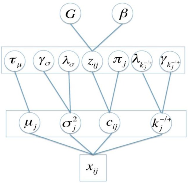
The graphical model representation of the proposed network model.

MCMC simulations

We carry out posterior inference for model (4) using MCMC simulations. Each iteration of the MCMC scheme includes the following transition probabilities,

$$\begin{array}{c}p(x|X,\pi ,\theta ,\beta ,G),p(c|\pi ,z),p(\pi |c),\\ p(\theta |X,c),p(\beta |z,G),p(G|z,\beta ).\end{array}$$

We start by generating Z_ij from its complete conditional posterior. Following the update of z, we generate values for c from complete conditional posterior p(c | π, z). If z_ij= 0, the update is deterministic, c_ij = −1. If z_ij = 1, the update requires a Bernoulli draw for c_ij = 0 versus c_ij = 1. The update of parameter θ is straightforward. Resampling G and the regression coefficients β could be challenging in large graphs, essentially because of the difficult evaluation of the normalization constant p(0 | β, G) in (3).²¹ For small graphs, which means that the number P of features in one single network is smaller than 12, we calculate the normalization constant p(0 | β, G) directly since p(G) is only supported over 2^P possible graphs, making the evaluation of the normalization constant straightforward. Thus, resampling G and β reduces to straightforward transdimensional MCMC as in Ref. 22. When P > 12, we implement an importance sampling estimate²¹ to approximate the ratio of the normalizing constants required for the evaluation of acceptance probabilities in the Metropolis–Hastings steps to update β and G.

FDR for edge inclusion

Statistically, owing to our fully model-based inference using posterior probabilities, we can easily assess the noise associated with the genomic data. This is a major advantage of our proposed Bayesian modeling approach over other algorithm-driven methods. Adopting the methods introduced by Newton et al.²³ and Müller et al.¹⁴, we compute the FDR for a given cutoff β₀, given by

$$\text{FDR}({\beta }_0)=\frac{{\displaystyle {\sum }_{u=1}^P{\displaystyle {\sum }_{w>u}(1-{\widehat{\beta }}_{uw})I({\widehat{\beta }}_{uw}\le {\beta }_0)}}}{{\displaystyle {\sum }_{u=1}^P{\displaystyle {\sum }_{w>u}I({\widehat{\beta }}_{uw}\le {\beta }_0)}}},$$

where I() is the indicator function, ${\widehat{\beta }}_{uw}$ is the posterior mean of β_uw in (3). We use 0.01 for the cutoff on FDR to call significant edges in the analyses.

Simulation Study

To evaluate the proposed model, we examined the performance of our model with three simulated data sets, each with N = 300 samples and P = 4,5,6 features, respectively. For each of the three simulations, a simulation truth G was first generated. For each pair of nodes {u,w}, we included the edge with a probability 0.5. For each imputed edge {u,w}, we generated values of β_uw from N(µ₁, 0.5²), µ₁ ∼ U(−4, 4). For the autologistic intercepts j, we first generated β_j from N(µ₂,0.5²), µ₂ ∼ U(−0.4, 0.4), and subsequently generated z for N = 300 samples. Since p(c_ij | z_ij = 0) = δ₋₁(c_ij), p(c_ij = 0|π_j, z_ij= 1) = π_j, and p(c_ij = 1|π_j,z_ij= 1) = 1 − π_j, we first generated π_j ∼ U(0.2,0.8), and then generated c. Furthermore, we let µ_j = 0, σ_j = 0.548, k_j− = 4, and k_j+ = 4 for each node. The hyper-parameters were fixed and set at τ_µ = 1, γ_σ = 2, λ_σ = 0.3, γ_k+ = 11, λ_k+ = 40, γ_k− = 11, λ_k− = 40, and σ_β = 3.

We implemented our model to compute the posterior summaries for each simulated data set. The posterior estimates were obtained by MCMC posterior simulation with 20,000 iterations, of which 6,000 are burn-in thinned by 10. This left us 1,400 posterior samplers. The computations were completed in less than 30 seconds on a MacBook Pro with 3 GHz Intel Core i7. We calculated the posterior inclusion probability q_uw for each possible edge {u,w} that is connected in the graph, which is defined as

$$q_{uw}=\frac{1}{1400}{\displaystyle \sum I\left(\left\{u,w\right\}\in E\right)}$$

substituting the edge set E of the imputed graph for each iteration of the MCMC. We then estimated the posterior graph $\widehat{G}$ using the FDR control based on the criterion {q_uw > q₀}. The threshold q₀ was chosen such that the posterior expected FDR was smaller than 0.1. We also reported parameter estimates $\overline{\beta }=E(\beta |X)$ denoting the posterior mean for the autologistic coefficients.

Figure 2 plots the simulated true graphs and posterior estimated graphs for three simulated data sets. Edge colors black and red represent positive and negative relationships. The numbers next to edges stand for either the true β_uw values or the posterior mean. The estimated graphs based on posterior inference are identical to the simulation truth, and the posterior estimated ${\widehat{\beta }}_{uw}$ are close to the true values.

Figure 2.

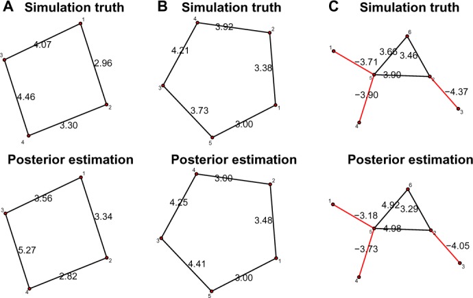
The simulation truth versus the estimated graph for three simulated data sets. Black edges represent positive relationship and red edges represent negative relationships. The number next to each edge represents either the true value or the posterior mean of the autologistic coefficients β_uws. (A) Data set 1; (b) data set 2; (C) data set 3.

Results

We implemented the proposed Bayesian graphical model and performed integrative inference based on BRCA and HNSC data described in BRCA and HNSC data section. We aim to discover the unknown dependence structure among different genomic features. The inference was obtained using the MCMC posterior simulation. The Markov chain included 20,000 iterations with 6,000 burn-in thinned by 10. The chain converged and mixed well. Three examples are showed in this section.

Multiple-genes network analysis

Transcription is an important genetic process in which DNA is transcribed to RNA. Perturbation of transcription may affect GE, and hence the subsequent protein production, leading to pathological states. Using the measurements of GE, CN and ME, one can learn the potential regulations within and between genes.

We chose two famous pathways including the MTOR signaling pathway and the p53 signaling pathway to show the posterior inference.

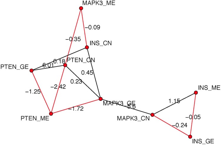
We selected measurements of GE, CN, and ME of three genes PTEN, INS, and MAPK in MTOR signaling pathway in BRCA data. So, the graph has nine nodes. Figure 3 shows the posterior estimated network. Edge colors black and red represent positive and negative relationships, respectively. The numbers next to edges stand for the posterior mean of autologistic coefficient β_uw. We find for gene PTEN, GE is positively related to CN and negatively related to ME, which is consistent with the biology finding that usually CN is positively related to GE while DNA ME is negatively related to GE. Similarly, GE and CN have positive relationship within gene MAPK3. In addition, given CN and GE of gene MAPK3, ME and GE of gene INS are conditionally independent with all other features.

Figure 3.

The posterior estimated graph for GE, CN, and ME of three genes PTEN, INS, and MAPK in MTOR signaling pathway in BRCA data. Black edges represent positive relationship and red edges represent negative relationships. The number next to each edge represents the posterior mean of the autologistic coefficients β_uws.

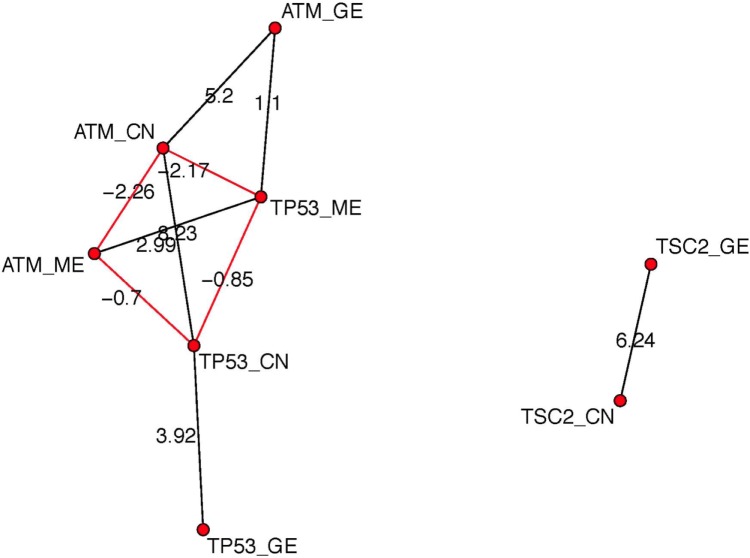
For p53 signaling pathway, we chose features GE, CN, and ME of genes ATM, TP53, and features GE, CN of TSC2. Thus, our network has eight nodes. Figure 4 shows the posterior estimated network. Within one single gene, we can observe that CN is positively related to GE, while ME is negatively related to GE, which agrees with known biology knowledge. There is no edge between features of gene TSC2 and features of other two genes TP53 and ATM, indicating that TSC2 functions independently with TP53 and ATM.

Figure 4.

The posterior estimated graph for GE, CN, and ME of three genes ATM, TP53, and TSC2 in p53 signaling pathway in BRCA data. Black edges represent positive relationship and red edges represent negative relationships. The number next to each edge represents the posterior mean of the autologistic coefficients β_uws.

Cancer-specific network analysis

A main goal of the proposed network model is to learn the cancer-specific networks so that the constructed networks can be used for the identification of different cancer types.

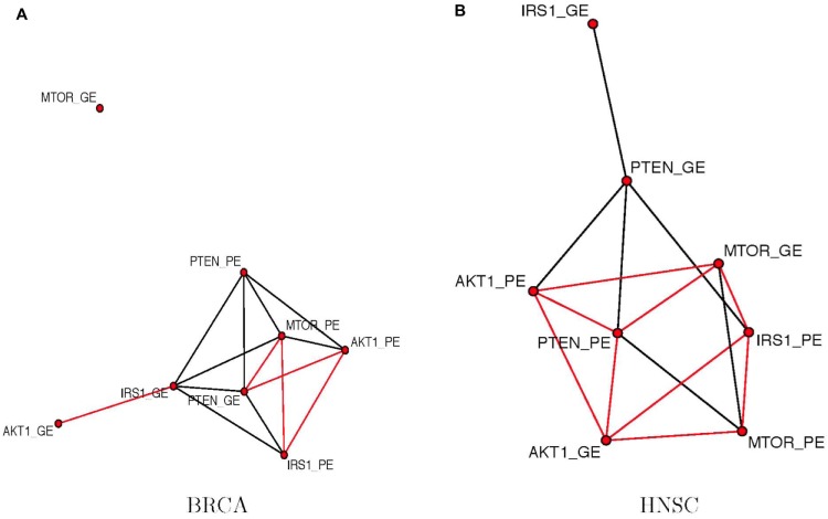
We selected two features GE and PE of four genes MTOR, IRS1, PTEN, and AKT1 in two different cancer types – BRCA and HNSC. All four genes function in MTOR signaling pathway. Figure 5 plots the posterior estimated graph. Comparing Figure 5A and B, we observe similarities and differences. In both cancer types, PE of gene MTOR is actively connected to other features. However, in BRCA, GE of MTOR does not have an edge with any other features, while in HNSC, GE of MTOR has an edge with four other features. Three of them are negative relationships. We observed edges consistent with existing understanding about the pathway. For example, PE of MTOR has a positive edge with PE of AKT1 in BRCA, which is consistent with the fact that MTOR is an activator of AKT1. Also, in HNSC, PE of PTEN has a negative edge with PE of AKT1 showing the effect of PTEN as an indirect repressor of AKT1 through PIP3 and PDK1. However, this edge becomes positive in BRCA condition indicating perturbations to MTOR signaling pathway in breast cancer. Comparing the topologies between two networks in different cancer types will be an interesting future direction.

Figure 5.

The posterior estimated graphs of features (GE and PE) among genes MTOR, IRS1, PTEN, and AKT1 in two different cancer types. Black edges represent positive relationship and red edges represent negative relationships. (A) BRCA and (b) HNSC.

Discussion and Conclusion

To study dependence structure of different genomic features within genes and between genes, we propose a Bayesian graphical model. The inferred graph gives a clear representation of the regulatory relationships. For example, GE of MTOR is positively related to PE of MTOR, but negatively related to PEs of AKT1, PTEN, and IRS1 in MTOR signaling pathway in HNSC. Our model can be easily applied to more features to learn the regulation relationship between features of different genes. For example, gene A could be a transcription factor for gene B if we detect a strong relationship between PE of gene A and mRNA expression of gene B. The proposed graphical model can well integrate multimodal genomic data from TCGA, including GE, PE, DNA ME, and gene CN, as shown in the analyses. It can also work on miRNA expression data, and we will extend the model to integrate DNA mutation data. In addition, we plan to implement the module linking the network topology with patient survival as a future extension. We are making a comprehensive list of these relationships using the entire TCGA data, expanding the effort to include more cancer types and more features such as microRNA and transcription factor. It is important to note that some interactions (such as CN–ME interactions) computationally derived by our proposed model might not be physical interactions, but could be indirect interactions through potentially multiple signaling steps that are not included in the current analysis. Confounding factors not included in analysis model can also contribute to the identified interactions. Nonetheless, we believe that the Bayesian graphical model will benefit researchers in different areas because of its rigor in statistical modeling for inferring interaction networks based on TCGA data.

REFERENCES

- 1.The Cancer Genome Atlas Network Comprehensive genomic characterization defines human glioblastoma genes and core pathways. Nature. 2008;455(7216):1061–8. doi: 10.1038/nature07385. [DOI] [PMC free article] [PubMed] [Google Scholar]
- 2.The Cancer Genome Atlas Network Comprehensive molecular portraits of human breast tumours. Nature. 2012;490(7418):61–70. doi: 10.1038/nature11412. [DOI] [PMC free article] [PubMed] [Google Scholar]
- 3.Jonsson PF, Bates PA. Global topological features of cancer proteins in the human interactome. Bioinformatics. 2006;22(18):2291–7. doi: 10.1093/bioinformatics/btl390. [DOI] [PMC free article] [PubMed] [Google Scholar]
- 4.Xu J, Li Y. Discovering disease-genes by topological features in human protein–protein interaction network. Bioinformatics. 2006;22(22):2800–5. doi: 10.1093/bioinformatics/btl467. [DOI] [PubMed] [Google Scholar]
- 5.Li Y, Liang M, Zhang Z. Regression analysis of combined gene expression regulation in acute myeloid leukemia. PLoS Comput Biol. 2014;10(10):e1003908. doi: 10.1371/journal.pcbi.1003908. [DOI] [PMC free article] [PubMed] [Google Scholar]
- 6.Friedman N, Linial M, Nachman I, Pe’er D. Using Bayesian networks to analyze expression data. J Comput Biol. 2000;7(3–4):601–20. doi: 10.1089/106652700750050961. [DOI] [PubMed] [Google Scholar]
- 7.Development Network, Schreiber SL, Shamji AF, et al. Towards patient-based cancer therapeutics. Nat Biotechnol. 2010;28(9):904–6. doi: 10.1038/nbt0910-904. [DOI] [PMC free article] [PubMed] [Google Scholar]
- 8.Waaijenborg S, de Witt Hamer V, Philip C, Zwinderman A. Quantifying the association between gene expressions and DNA-markers by penalized canonical correlation analysis. Stat Appl Genet Mol Biol. 2008;7(3) doi: 10.2202/1544-6115.1329. Article3. [DOI] [PubMed] [Google Scholar]
- 9.Menezes RX, Boetzer M, Sieswerda M, Van Ommen GJB, Boer JM. Integrated analysis of DNA copy number and gene expression microarray data using gene sets. BMC Bioinformatics. 2009;10(1):203. doi: 10.1186/1471-2105-10-203. [DOI] [PMC free article] [PubMed] [Google Scholar]
- 10.Choi H, Qin ZS, Ghosh D. A double-layered mixture model for the joint analysis of DNA copy number and gene expression data. J Comput Biol. 2010;17(2):121–37. doi: 10.1089/cmb.2009.0019. [DOI] [PMC free article] [PubMed] [Google Scholar]
- 11.Etcheverry A, Aubry M, De Tayrac M, et al. DNA methylation in glioblastoma: impact on gene expression and clinical outcome. BMC Genomics. 2010;11(1):701. doi: 10.1186/1471-2164-11-701. [DOI] [PMC free article] [PubMed] [Google Scholar]
- 12.Shen R, Olshen AB, Ladanyi M. Integrative clustering of multiple genomic data types using a joint latent variable model with application to breast and lung cancer subtype analysis. Bioinformatics. 2009;25(22):2906–12. doi: 10.1093/bioinformatics/btp543. [DOI] [PMC free article] [PubMed] [Google Scholar]
- 13.Li W, Zhang S, Liu CC, Zhou XJ. Identifying multi-layer gene regulatory modules from multi-dimensional genomic data. Bioinformatics. 2012;28(19):2458–66. doi: 10.1093/bioinformatics/bts476. [DOI] [PMC free article] [PubMed] [Google Scholar]
- 14.Müller P, Parmigiani G, Robert C, Rousseau J. Optimal sample size for multiple testing. J Am Stat Assoc. 2004;99(468):990–1001. [Google Scholar]
- 15.Setty M, Helmy K, Khan AA, et al. Inferring transcriptional and microRNA-mediated regulatory programs in glioblastoma. Mol Syst Biol. 2012;8(1):605. doi: 10.1038/msb.2012.37. [DOI] [PMC free article] [PubMed] [Google Scholar]
- 16.Tibshirani R. Regression shrinkage and selection via the lasso. J R Stat Soc Series B. 1996;58:267–88. [Google Scholar]
- 17.Parmigiani G, Garrett ES, Anbazhagan R, Gabrielson E. A statistical framework for expression-based molecular classification in cancer. J R Stat Soc Series B Stat Methodol. 2002;64(4):717–36. [Google Scholar]
- 18.Besag J. Spatial interaction and the statistical analysis of lattice systems. J R Stat Soc Series B. 1974;36:192–236. [Google Scholar]
- 19.Caragea PC, Kaiser MS. Autologistic models with interpretable parameters. JABES. 2009;14(3):281–300. [Google Scholar]
- 20.Hughes J, Haran M, Caragea PC. Autologistic models for binary data on a lattice. Environmetrics. 2011;22:374–8. [Google Scholar]
- 21.Mitra R, Müller P, Liang S, Yue L, Ji Y. A Bayesian graphical model for chip-seq data on histone modifications. J Am Stat Assoc. 2013;108(501):69–80. [Google Scholar]
- 22.Green PJ. Reversible jump Markov chain Monte Carlo computation and Bayesian model determination. Biometrika. 1995;82(4):711–32. [Google Scholar]
- 23.Newton MA, Noueriry A, Sarkar D, Ahlquist P. Detecting differential gene expression with a semiparametric hierarchical mixture model. Biostatistics. 2004;5:155–76. doi: 10.1093/biostatistics/5.2.155. [DOI] [PubMed] [Google Scholar]