Mapping Activity Patterns to Quantify Risk of Violent Assault in Urban Environments

Supplemental Digital Content is available in the text.

Background:

We collected detailed activity paths of urban youth to investigate the dynamic interplay between their lived experiences, time spent in different environments, and risk of violent assault.

Methods:

We mapped activity paths of 10- to 24-year-olds, including 143 assault patients shot with a firearm, 206 assault patients injured with other types of weapons, and 283 community controls, creating a step-by-step mapped record of how, when, where, and with whom they spent time over a full day from waking up until going to bed or being assaulted. Case–control analyses compared cases with time-matched controls to identify risk factors for assault. Case-crossover analyses compared cases at the time of assault with themselves earlier in the day to investigate whether exposure increases acted to the trigger assault.

Results:

Gunshot assault risks included being alone (odds ratio [OR] = 1.6, 95% confidence interval [CI] = 1.3, 1.9) and were lower in areas with high neighbor connectedness (OR = 0.7, 95% CI = 0.6, 0.8). Acquiring a gun (OR = 1.4, 95% CI = 1.1, 1.6) and entering areas with more vacancy, violence, and vandalism (OR = 1.7, 95% CI = 1.1, 2.7) appeared to trigger the risk of getting shot shortly thereafter. Nongunshot assault risks included being in areas with recreation centers (OR = 1.2, 95% CI = 1.1, 1.4). Entering an area with higher truancy (OR = 1.6, 95% CI = 1.1, 2.5) and more vacancy, violence, and vandalism appeared to trigger the risk of nongunshot assault. Risks varied by age group.

Conclusions:

We achieved a large-scale study of the activities of many boys, adolescents, and young men that systematically documented their experiences and empirically quantified risks for violence. Working at a temporal and spatial scale that is relevant to the dynamics of this phenomenon gave novel insights into triggers for violent assault.

Gunshot violence is the leading cause of death in 10- to 24-year-old African American males and the second leading cause of death among 10- to 24-year-olds overall in the United States.¹ For each adolescent that dies of a gunshot assault, five more will survive, undergoing extensive treatment in hospital emergency departments.^1,2 These assaults are predominantly an urban phenomenon.³

Whereas their minute-to-minute activities and locations influence the likelihood that adolescents will engage in risky behaviors and be exposed to violence-prone locations and environments, the precise mechanisms and details of this influence have been elusive.^4–9 The best insights from multiple disciplines suggest that youth violence is the end result of a web¹⁰ of factors that include alcohol use, access to firearms, and disadvantaged urban environments.^4,11–19 Most investigations of youth violence have used ecologic or cross-sectional designs, however, and thus could not scrutinize the observed effects relative to a strong counterfactual. A related limitation is that tests of a causal hypothesis ideally would allow for a time interval between exposure and disease onset that corresponds to a meaningful induction period.²⁰ Thus, while the best evidence suggests that a range of youth behaviors and urban environments correlate with violence, the factors that should be prioritized for targeted interventions are unknown.

We sought to fill this gap in knowledge through detailed space-time modeling of the step-by-step movement of individuals through an urban landscape over time, estimating their risks of violence relative to the people, places, and situations they encounter.

METHODS

Overview

We conducted the Space-Time Adolescent Risk Study in Philadelphia, Pennsylvania. Essentially, we aimed to obtain and then join data of two types: the step-by-step latitude and longitude coordinates of routes that young people travelled, and the social and structural aspects of the locations each person traversed or spent time.

Recruitment and Enrollment

Enrollment followed a population-based case–control study approach. The case subjects were 10- to 24-year-old males who sustained an injury from violence. We enrolled these assaulted individuals into one of two case subject groups according to their injury type: a gunshot wound, or an injury other than a gunshot wound (e.g., laceration, contusion, or fracture from being hit, struck with object, etc.). The cases were recruited from the emergency departments of a pediatric and an adult level I trauma center located adjacently in central Philadelphia. A control group of 10- to 24-year-old males was recruited from households in the 12 ZIP code hospital catchment area using random digit dialing to residential telephones (see eAppendix 2 for details; http://links.lww.com/EDE/A975). All participants were enrolled using informed consent or, for minors, assent with parental informed consent. The study was approved by the University of Pennsylvania institutional review board.

Interview and Collection of Space-time Activity Data

Case and control subjects were interviewed in person at our research office, at the subject’s home, or in the hospital. The interview included administering a questionnaire about demographics, health, school performance, relationships with friends and family, risk-taking behaviors, perspectives about the area where they live, and standardized instruments (see eTable 1, listing the questions; http://links.lww.com/EDE/A975).

The interview also involved collecting a detailed record of the subject’s recent activities. Cases referred to the day of the assault; respondents in the control sample were asked to refer to a recent day (within 3 days of the interview) designated at random. While seated side-by-side, the data were collected by entering the subject’s detailed report of their activities into a geographic information system application developed for this study (see eFigure1, showing a screenshot; http://links.lww.com/EDE/A975). Details of methods to collect and process the data are provided in eAppendix 2 (http://links.lww.com/EDE/A975).

Measuring the Landscape of Each Subject’s Activities

We accessed geographic data including characteristics of streets, buildings, and neighborhood populations from the University of Pennsylvania Cartographic Modeling Lab. Using kernel density methods for point data and inverse-distance weighing methods for polygon data, each variable was transformed into a raster data surface layer that spanned the entire surface area of Philadelphia and was expressed as a continuous variable.²¹

Seven of the geographic variables were based on residents’ responses to a regional household telephone interview. For example, the variable “improve” was derived by asking “Have people in your neighborhood ever worked together to improve the neighborhood? For example, through a neighborhood watch, creating a community garden, building a community playground, or participating in a block party” (see eTable 2, listing data sources and question wording; http://links.lww.com/EDE/A975).

Having geographically referenced data with a high level of geographic specificity for the entire city of Philadelphia, the map layers represent the prevalence of risk factors and protective factors present at any specific location. By appending these data of the environment to the activity path data by latitude and longitude coordinates of subjects’ activities, we derived estimates, with high geographic and temporal specificity, of the exposure history experienced by each subject over their daily activities. We also appended each path point with climate data to indicate the temperature, whether it was precipitating, and whether each point of each subject’s activities occurred during daylight or dark.

Factor Analysis

With 27 environmental variables, we would likely encounter multicollinearity in regressions designed to comprehensively control for environmental context. Thus, after appending the variables to the subject paths, we conducted factor analysis on the 27 variables and derived composite factors that efficiently represented the underlying constructs.²²

Descriptive Statistics

We used descriptive statistics to compare each case subject group with the control subject group. We generated figures to evaluate the percent of subjects’ activities spent in different types of activities and modes of transportation. Also, we investigated variability in the extent that subjects became exposed to features of the environment as they carried out daily activities (see eAppendix 2 for details; http://links.lww.com/EDE/A975).

Regression Analysis

We conducted two sets of regression analyses to derive estimates, in the form of odds ratios and 95% confidence intervals, of whether characteristics of individuals, their activities and their immediate context, and characteristics of the locations where they spent time protected against or posed a risk for young people to be assaulted.

In part 1, we estimated whether cases, at the time they were assaulted, differed from time-of-day matched observations on controls. This was accomplished by following a matched case–control analysis approach, using a conditional logistic regression model, and using only one observation to represent each case subject—the point when they were assaulted—and using all observations for each control subject. We stratified the model by time of day according to seven strata representing morning, afternoon, evening, and nighttime hours. In this way, each case subject’s exposure levels at the time they were assaulted were compared with the exposure levels experienced by controls at the same time of day that the particular case was assaulted.

Covariates in the model included characteristics of subjects, indicators of their activities and immediate context, and characteristics of their environment. Subject age was included as a covariate to control for age variability between cases and controls within the age-group strata used for recruitment. Variables indicating day of week, month, and date- and hour-specific precipitation were included to control for potential confounding. Each of the indicators of the built and social environment was modeled in its standardized form. Thus, the odds ratios are interpreted as the estimated relative risk of assault associated with a one standard deviation unit increase in the exposure. We used robust standard errors and stratified the model by age group to investigate effect modification.

Part 2 used the dataset that represented the entire span of subjects’ daily activities. We followed a case-crossover design to derive estimates of whether any of the exposures that we were interested in were intermittent and served to trigger the onset of assault.²³ This was accomplished by determining whether cases, at the time they were assaulted, were engaged in new activities as compared with earlier in the day, or were exposed to environmental variables at a level that differed from what they experienced earlier that day. To do this, we had one approach to manage dichotomous variables, like the indicator of whether the subject was carrying a gun at a given time (yes = 1, no = 0), and another approach to manage continuous environmental variables, like the prevalence of recreation centers in the location of the subject at a given time.

For each case subject, we identified whether the case was coded yes or no on each dichotomous (binary) variable at each point of their activity path, and from that value we subtracted the mean of the values on that variable that were observed among controls at the same time of day. For example, if a case had been carrying a gun at 7:20 pm (originally coded 1) and 40% of the controls had been carrying a gun at 7:20 pm, the new variable representing gun possession by that case subject was coded 0.6 (because the mean of a binary variable coded 1 for 40% of control subjects is 0.4, and 1–0.4 = 0.6). If the case had not been carrying a gun at 9:10 am (originally coded 0) and 10% of the controls had been carrying a gun at 9:10 am, the new variable representing gun possession by the case subject was coded −0.1 (because 0–0.1 = −0.1). For the continuous environmental variables, we identified the case subject’s level of exposure to each environmental variable at each point of their activity path, and from that value we subtracted the mean of the time-specific values that we had calculated on that variable among controls at that time of day. In this way, we differenced the time series of each case subject by the time-of-day-specific levels of exposures experienced by controls.

The analysis of these data used conditional logistic regression with robust standard errors and entailed comparing each case subject’s exposure status at the time they were assaulted (i.e., during the last 10 minutes of their activity path) to their own level of exposure at each point (i.e., during each 10- minute interval) earlier in the day. In this way, we were treating the hazard period as the 10 minutes leading up to and including the time of the assault.²³ When applied to the differenced exposure variables, this differenced case-crossover study carried out a difference-in-differences analysis. The models were stratified by age group to gauge effect modification. We also carried out a traditional (i.e., not differenced) case-crossover analysis as a robustness check.

RESULTS

Characteristics of Subjects

We enrolled 632 subjects, including 143 gunshot case subjects, 206 nongunshot case subjects, and 283 control subjects from among 250, 396, and 496 eligible individuals who were recruited, respectively. The enrolled case subjects did not differ from eligible patients who were not enrolled in terms of age, race, time of presenting to the emergency department, duration of time to be triaged, whether they were admitted to the hospital, or location of assault.

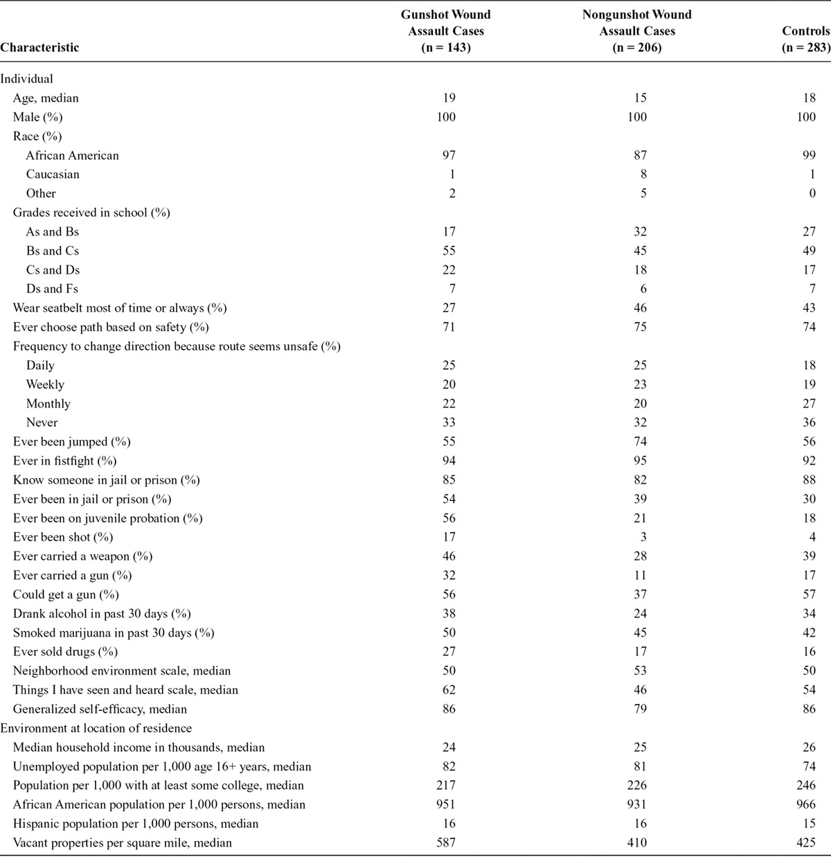
Table 1 reports subject characteristics, based on location of residence and baseline survey responses. As planned, all subjects were male. Compared with the controls, neither case group differed in grades received in school. Nongunshot cases, but not gunshot cases, were more likely than controls to frequently change direction as they walked due to feeling that their environment seemed unsafe. A greater proportion of nongunshot cases compared with controls had been “jumped” in the past, whereas a greater proportion of gunshot cases compared with controls had spent time in jail or prison or on juvenile probation. Four percent of controls and 3% of nongunshot cases had been shot before, and 17% of the gunshot case subjects had previously been shot. The areas where subjects’ homes were located were similar in median household income, unemployment rate, and prevalence of Hispanic population. See eAppendix 3 for a discussion of additional comparisons (http://links.lww.com/EDE/A975).

TABLE 1.

Characteristics of 10- to 24-Year-old Subjects

Factor Analysis

The factor analysis derived six factors and left over four variables that did not load on any of the factors (see eTable 3, showing results; http://links.lww.com/EDE/A975). The six factors represented constructs corresponding to connectedness among neighbors, income, alcohol outlets and drunkenness and disorderly conduct, vacant lots and vandalism and violence, fire stations and police stations, and race and ethnicity (where higher values correspond to a higher proportion of Hispanic residents and a lower proportion of African American residents). The remaining four variables were prevalence of household gun ownership, proportion of the population 15–24 years old, prevalence of recreation centers, and truancy rate in schools.

Activity Path Analysis

Dynamics in Modes of Transportation and Places of Daily Activities

Figure 1 shows stark variability in the percent of time during each hour that gunshot cases, nongunshot cases, and controls, respectively, spent in different types of places and modes of transportation. These findings communicate that the nature and location of activities varies dynamically across the course of daily activities and is evidence that such variability will be important to account for if we hope to understand assault risks that are associated with the context and nature of activities in the urban landscape (see eFigures 2 and 3 for supplementary findings; http://links.lww.com/EDE/A975).

FIGURE 1.

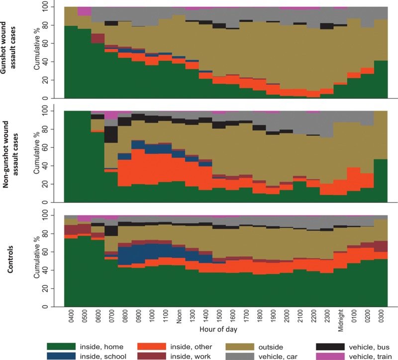
Percent of time during each hour of the day that subjects (all ages) spent in different types of locations and modes of transportation, by subject group.

Dynamics of Exposure Levels During Travel Across Urban Landscape

Raster map layers shown in Figure 2 indicate the levels of exposure of 27 features of the built and social environment across the urban landscape of the city. Each layer is immediately informative in that reveals the extent to which levels of exposure vary by location.

FIGURE 2.

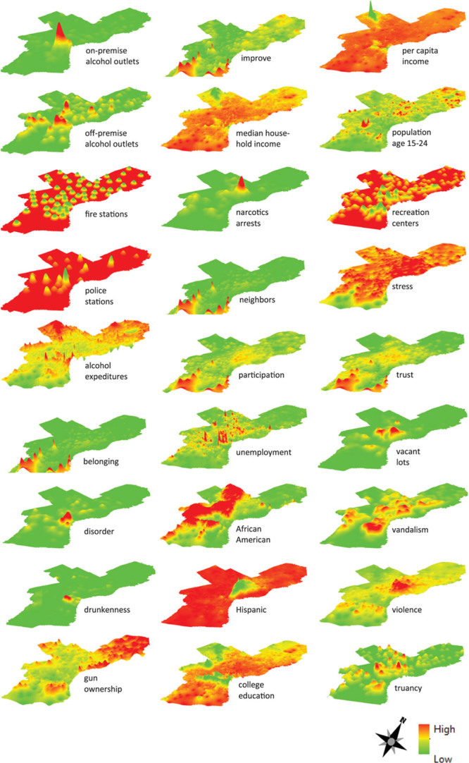
Raster surface layer of the 27 risk factors and protective factors across the urban landscape.

Figure 3 shows how subjects’ paths were overlaid upon the raster map layers, as demonstrated for all 632 subjects with respect to off-premise alcohol outlets as an example, to determine the levels of exposure that were encountered over daily activities.

FIGURE 3.

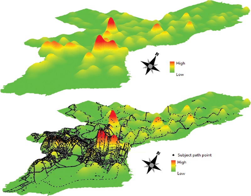
Raster surface layer of the level of a risk factor in the urban landscape as demonstrated using off-premise alcohol outlets (top). Raster surface layer of the urban landscape overlaid with path points marking locations of the daily activities of 632 study subjects (bottom).

Part 1 Regression

Individual Context and Environmental Exposures at Time of Assault

Table 2 reports regression results comparing gunshot case subjects and nongunshot case subjects at the location and time when they were assaulted to data on time-matched controls. Results varied by age group. Using this approach, among older subjects (ages 18 years and older; see eTable 4; http://links.lww.com/EDE/A975), the risk of gunshot assault was higher when subjects were alone, was higher when it was precipitating, and was higher when outdoors on foot and lower when riding a bus or trolley than when indoors. Also, the risk of gunshot assault was higher in areas with high levels of vacant properties and vandalism and violence, higher in areas with fire and police stations, and higher in areas with a high prevalence household gun ownership. The risk of gunshot assault was lower in areas with high levels of neighbor connectedness and with a high prevalence of Hispanic population and low prevalence of African American population. Among younger subjects (ages less than 18 years; see eTable 4; http://links.lww.com/EDE/A975), the risk of gunshot assault was higher when outdoors on foot and when using motorized transportation and lower when riding a bus or trolley than when indoors. Also, the risk of gunshot assault was higher when in areas of high household income, higher in areas with fire and police stations, and high levels of household gun ownership.

TABLE 2.

Results of Adjusted Case-control Analysis Comparing Gunshot and Nongunshot (All Ages) Case Subjects’ Levels of Exposure to Individual and Situational Circumstances, Climate Characteristics, and Environmental Contexts at the Time of Being Assaulted Relative to Time-matched Controls

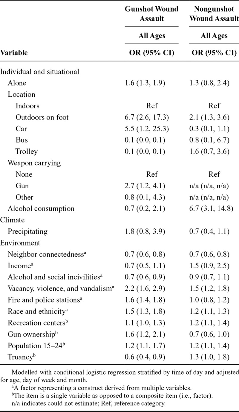
The results of the nongunshot assault analysis on subjects overall are shown in Table 2 as noted above. Among older subjects (see eTable 4; http://links.lww.com/EDE/A975), the risk of nongunshot assault was higher when riding a trolley compared with when indoors and was higher when consuming alcohol. Also, the risk of nongun assault was higher in areas with high levels of vacant properties and vandalism and violence. The risk of nongun assault was lower in areas with high levels of neighbor connectedness. Among younger subjects (see eTable 4; http://links.lww.com/EDE/A975), the risk of nongun assault was higher when outdoors on foot and was lower when riding a trolley compared with when indoors. Also, the risk of nongun assault was higher in areas with high levels of vacant properties, violence, and vandalism, and with recreation centers. The risk of nongun assault among younger subjects was also lower when it was precipitating and lower in areas of high neighbor connectedness.

The part 1 regression results do not account for the possibility that cases, and controls, experienced varying levels of exposure during their daily activities. Supplementary analyses (see eFigures 4 and 5, showing results; http://links.lww.com/EDE/A975) found that considerable variability did occur (also see description in eAppendix 3; http://links.lww.com/EDE/A975). The part 2 regression analyses investigate whether changes in exposure levels triggered the onset of assault.

Part 2 Regression

Triggers for Assault Based on Contexts and Environments of Daily Activities

Table 3 reports that young people were shot at a time when they were in different activities as compared with earlier in the day, and when in an extreme location, in that the prevalence of several risk factors and protective factors was considerably higher or lower in that location as compared with the locations where the subject spent time earlier that day. Results varied by age group. Using this approach, we found that older individuals (ages 18 years and older; see eTable 5; http://links.lww.com/EDE/A975) faced an elevated risk to be shot when they were outdoors on foot or when in a car, bus, or trolley as compared with when indoors. The risk was also higher when carrying a gun. Also, they faced an elevated risk to be shot when in an area that was high in vacancy and vandalism and in violence. We found that younger individuals (ages less than 18 years old; see eTable 5; http://links.lww.com/EDE/A975) faced an elevated risk to be shot when it was precipitating and when outdoors on foot or in a car, bus, or trolley as compared with when indoors.

TABLE 3.

Results of Adjusted Case-crossover Analysis Comparing Gunshot and Nongunshot (All Ages) Case Subjects’ Levels of Exposure to Individual and Situational Circumstances, Climate Characteristics, and Environmental Contexts at the Time of Being Assaulted Relative to Times Preceding the Assault

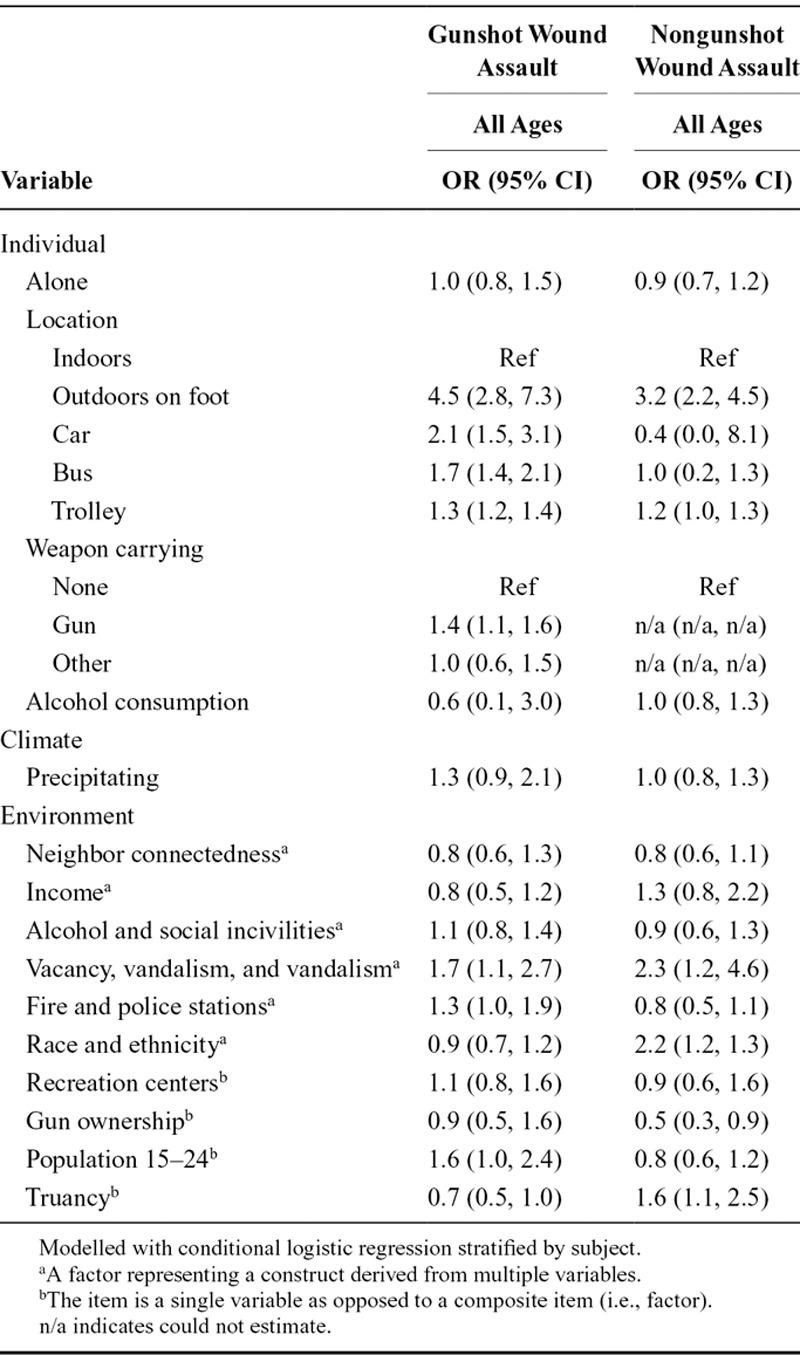
Regarding the risk of nongun assault, we found that older individuals faced an elevated risk to be assaulted with a nongun weapon when outdoors on foot or when riding a trolley as opposed to indoors (see eTable 5; http://links.lww.com/EDE/A975). Also, they faced an elevated risk to be assaulted when in an area with high household income or high in vacant properties and vandalism and in violence. Younger individuals faced an elevated risk to be assaulted with a nongun weapon when outdoors on foot as opposed to indoors and when in an area that was high in truancy (see eTable 5; http://links.lww.com/EDE/A975). They faced a lower risk to be assaulted when in an area high in gun ownership.

The approach that used a basic case-crossover analysis produced odds ratios that were generally larger (further from the null) for both risk factors and for protective factors (not reported). Thus, we preferred the differenced approach given that it appeared to produce conservative results.

DISCUSSION

By developing a new approach for studying the dynamics of activities in an urban environment, we found that the context of young people’s activities and characteristics of the places they spent time put them at risk to be assaulted or protected them from being assaulted, and certain activities appeared to trigger the onset of assault. Whereas in One Boy’s Day, Barker and Wright observed sequences of events play out as one research subject navigated his environment and encountered situations that could compromise his health,⁷ we achieved a large-scale study of the activities of many boys, adolescents, and young men that systematically documented their experiences and empirically quantified risks for violence (see eAppendix 1, for further discussion; http://links.lww.com/EDE/A975).

We found that individuals’ activities were constrained in space and time²⁴ as a function of their daily routines, and those who were assaulted differed considerably from those who were not assaulted in terms of the amount of time they spent in different types of activities, locations, and modes of transportation. The part 1 regressions suggested that individuals who are assaulted differ from others in terms of being chronically (i.e., generally) exposed to the conditions that were identified. The part 2 regressions enhanced our understanding of urban violence by revealing that engaging in certain activities and coming into contact with certain types of locations seemed to act as triggers that abruptly resulted in assault.

Of the numerous neighborhood conditions that we found to be associated with violence, we are most encouraged by identifying that structural features of the environment including recreation centers, alcohol outlets, and vacant properties were associated with a risk of violence. Others have suggested that each of these is potentially modifiable, and vacant properties in particular could be ameliorated with structural, scalable, and sustainable interventions²⁵ that could help make neighborhoods safer.^25,26

A key strength of this study was using a momentary analysis of activities rather than an individual-level analysis as is common in epidemiology research. Indeed, Chaix et al.²⁷ recently pointed out the importance of advancing past a typical approach that takes into account only residential neighborhoods in the definition of exposure, to studying the impact of mobility and health, and the importance of developing new methods to make this possible. One approach that is emerging quickly uses global position systems (GPS) to monitor the locations of activities, and incorporates ecologic momentary assessments to reveal valuable new insights about participants’ activities (e.g., smoking, physical activity) in relation to contexts and their locations. Note that a GPS approach is typically prospective in nature. Thus, GPS is well suited to study exposures and outcomes that occur frequently enough during a time frame during which subjects can reasonably be expected to participate. Our outcome of interest, the assault of an adolescent, despite occurring so frequently in the study setting, is a statistically rare event. Hence our motivation to use a case–control design, and hence our need to develop a new interview protocol and geographic information system mapping application to collect exposure information regarding subjects’ activities retrospectively, and measure mobility and the links between activities and exposures at a temporal and spatial scale that was relevant to the dynamics of the phenomenon under study. We hope our study will help motivate the emerging wave of research that Chaix et al. called for recently, and that Barker and Wright demonstrated 60 years ago in their seminal study of a single boy’s activities.

Our study yielded rich data that offer possibilities to study other important questions and to pursue next steps. In particular, we have the rare opportunity to investigate the length of the induction period for risk factors of adolescent assault. In our case-crossover analysis, the hazard period was defined as the 10 minutes preceding the assault.²³ Thus, we examined whether 10 minutes was the induction period for the covariates we investigated as potential risk factors. With no previous studies for insight, this was a reasonable starting assumption. For example, adolescents may dare to enter a high-risk situation shortly after acquiring a gun; adolescents may engage in conflict with other youth shortly after arriving at a recreation center. Alternatively, though, the induction period for each of these may be longer than 10 minutes. We have reserved a deeper investigation of this topic for separate study. Any bias from our use of a 10-minute window is expected to be toward the null.²³

Limitations

Nonparticipation bias could occur from issues with enrolling either case or control subjects. For one, controls were recruited only from homes with a landline telephone, whereas cases were recruited regardless of their telephone status. A potential concern is that income and telephone type may be related. Although we do not know how many of the case subjects did not have a landline telephone, we did report more direct evidence from the neighborhood data that cases and controls did not differ regarding income levels where they reside. This provides assurance that the controls did not differ systematically from the base population. Also, for case subjects, we enrolled only patients who survived an assault. We do not know whether assault victims who died during the study period differed from those who survived. Thus, not including decedents as cases could pose selection bias. We know of no literature or clinical evidence suggesting that a disparity exists systematically between urban violence assault victims who live versus die, however, and therefore feel that this threat to validity is minimal. Note that whereas some studies enroll deceased cases and interview a family member proxy, we believe that approach was not valid for collecting the detailed activity path data that we sought and that enabled the novel insights that we have reported here. Also, even among adolescent victims of assault by gunshot, approximately five of six victims survive, which further allays our concern of this potential bias.^1,2

Information bias from poor recall or untruthful responding is a threat to validity. However, control subjects’ responses to the baseline questions that were comparable with those administered to youth taking the Youth Risk Behavior Survey give evidence that our controls were like Pennsylvania youth in seatbelt use and substance use (see eAppendix 3, reporting results; http://links.lww.com/EDE/A975). Also, finding a high prevalence of socially undesirable behaviors on the baseline survey for both cases and controls is evidence that subjects were not underreporting. Ultimately it was the activity path data that we used to derive the effect estimates and there are indications those data are valid. Our primary aim investigated whether spending time around alcohol outlets, recreation centers, vacant lots, and other environmental features relate to assault risk. Yet we made no mention of these during the mapping exercise used to collect these data. We simply asked subjects to trace the route they travelled through their day. If we are correct that respondents would feel that little if any stigma would be attached to describing the route they travelled to the interviewer, this supports the possibility that the path data are valid. Also, face validity of the activity path data is evidenced by the figures of subjects’ activities by hour of day, indicating that by age group, the things that subjects reported doing made sense with respect to time of day. Also, we designed the entire recruitment and interview process to incorporate many features intended to assure subjects that their responses would be kept confidential.

Finally, most observed effects went in the hypothesized direction, but we did not expect to see neighborhood income relate positively to gunshot assault. Subsequent qualitative research could help interpret this finding.

Conclusion

We believe this is the first study to accomplish a momentary analysis of activities to elucidate specific mechanisms that put adolescents and young men at risk of violent assault. The results advance our understanding of violence, demonstrate the value of measuring momentary activities at a temporal and spatial scale that is meaningful to the relationships under study, and point to structural features of urban environments that can be targeted to make communities safer.

Supplementary Material

ede-27-032-s001.pdf ^{(1MB, pdf)}

REFERENCES

- 1.CDC. WISQARS Leading cause of death reports. 2009. [Google Scholar]
- 2.CDC. WISQARS Nonfatal Injury Reports. 2010. [Google Scholar]
- 3.Nance ML, Carr BG, Kallan MJ, Branas CC, Wiebe DJ. Variation in pediatric and adolescent firearm mortality rates in rural and urban US counties. Pediatrics. 2010;125:1112–1118. doi: 10.1542/peds.2009-3219. [DOI] [PubMed] [Google Scholar]
- 4.Rapp Paglicci LA, Wodarski JS. Antecedent behaviors of male youth victimization: an exploratory study. Deviant Behav. 2000;21:519–536. [Google Scholar]
- 5.Cherpitel CJ. Substance use, injury, and risk-taking dispositions in the general population. Alcohol Clin Exp Res. 1999;23:121–126. [PubMed] [Google Scholar]
- 6.Hertz-Picciotto I. Environmental epidemiology. In: Rothman KJ, Greenland S, editors. Modern Epidemiology. 2nd ed. Philadelphia, PA: Lippincott Williams & Wilkins; 1998. p. 557. [Google Scholar]
- 7.Barker RG, Wright HF. One Boy’s Day: A Specimen Record of Behavior. New York, NY: Harper & Brothers; 1951. [Google Scholar]
- 8.Anderson E. Code of the Street: Decency, Violence, and the Moral Life of the Inner City. New York, NY: W. W. Norton; 1999. [Google Scholar]
- 9.Christoffel KK. Violent death and injury in US children and adolescents. Am J Dis Child. 1990;144:697–706. doi: 10.1001/archpedi.1990.02150300095025. [DOI] [PubMed] [Google Scholar]
- 10.Mausner J. Epidemiology: An Introductory Text. Philadelphia, PA: WB Saunders; 1985. [Google Scholar]
- 11.Clark TA. Prevalence of drugs and alcohol in autopsied homicide cases in St. John Parish, Louisiana. J La State Med Soc. 1996;148:257–259. [PubMed] [Google Scholar]
- 12.Hlady WG, Middaugh JP. Suicides in Alaska: firearms and alcohol. Am J Public Health. 1988;78:179–180. doi: 10.2105/ajph.78.2.179. [DOI] [PMC free article] [PubMed] [Google Scholar]
- 13.Brent DA, Perper JA, Allman CJ. Alcohol, firearms, and suicide among youth. Temporal trends in Allegheny County, Pennsylvania, 1960 to 1983. JAMA. 1987;257:3369–3372. [PubMed] [Google Scholar]
- 14.Ford AB, Rushforth NB, Rushforth N, Hirsch CS, Adelson L. Violent death in a metropolitan county: II. Changing patterns in suicides (1959-1974). Am J Public Health. 1979;69:459–464. doi: 10.2105/ajph.69.5.459. [DOI] [PMC free article] [PubMed] [Google Scholar]
- 15.Rivara FP, Mueller BA, Somes G, Mendoza CT, Rushforth NB, Kellermann AL. Alcohol and illicit drug abuse and the risk of violent death in the home. JAMA. 1997;278:569–575. [PubMed] [Google Scholar]
- 16.DuRant RH, Kahn J, Beckford PH, Woods ER. The association of weapon carrying and fighting on school property and other health risk and problem behaviors among high school students. Arch Pediatr Adolesc Med. 1997;151:360–366. doi: 10.1001/archpedi.1997.02170410034004. [DOI] [PubMed] [Google Scholar]
- 17.Fingerhut LA, Ingram DD, Feldman JJ. Firearm homicide among black teenage males in metropolitan counties. Comparison of death rates in two periods, 1983 through 1985 and 1987 through 1989. JAMA. 1992;267:3054–3058. [PubMed] [Google Scholar]
- 18.Sheley JF, McGee ZT, Wright JD. Gun-related violence in and around inner-city schools. Am J Dis Child. 1992;146:677–682. doi: 10.1001/archpedi.1992.02160180035012. [DOI] [PubMed] [Google Scholar]
- 19.Wikström PH, Oberwittler D, Treiber K, Hardie B. Breaking Rules: The Social and Situational Dynamics of Young People’s Urban Crime. Oxford, England: Oxford University Press; 2013. [Google Scholar]
- 20.Greenland S. Applications of stratified analysis methods. In: Rothman KJ, Greenland S, Lash TL, editors. Modern Epidemiology. 3rd ed. Philadelphia, PA: Lippincott Williams & Wilkins; 2008. pp. 300–301. [Google Scholar]
- 21.Tomlin CD. Geographic Information Systems and Cartographic Modeling. Englewood Cliffs, NJ: Prentice-Hall; 1990. [Google Scholar]
- 22.Harman HH. Modern Factor Analysis. 3rd ed. Chicago, IL: University of Chicago Press; 1976. [Google Scholar]
- 23.Maclure M. The case-crossover design: a method for studying transient effects on the risk of acute events. Am J Epidemiol. 1991;133:144–153. doi: 10.1093/oxfordjournals.aje.a115853. [DOI] [PubMed] [Google Scholar]
- 24.Hägerstrand T. What about people in regional science? Pap Reg Sci Assoc. 1970;24:6–21. [Google Scholar]
- 25.Branas CC, MacDonald JM. A simple strategy to transform health, all over the place. J Public Health Manag Pract. 2014;20:157–159. doi: 10.1097/PHH.0000000000000051. [DOI] [PMC free article] [PubMed] [Google Scholar]
- 26.Maantay J. Zoning, equity, and public health. Am J Public Health. 2001;91:1033–1041. doi: 10.2105/ajph.91.7.1033. [DOI] [PMC free article] [PubMed] [Google Scholar]
- 27.Chaix B, Méline J, Duncan S, et al. Neighborhood environments, mobility, and health: towards a new generation of studies in environmental health research. Rev Epidemiol Sante Publique. 2013;61(Suppl 3):S139–S145. doi: 10.1016/j.respe.2013.05.017. [DOI] [PubMed] [Google Scholar]