

Abstract
Background
Drug poisoning mortality has increased substantially in the U.S. over the past 3 decades. Previous studies have described state-level variation and urban–rural differences in drug-poisoning deaths, but variation at the county level has largely not been explored in part because crude county-level death rates are often highly unstable.
Purpose
The goal of the study was to use small-area estimation techniques to produce stable county-level estimates of age-adjusted death rates (AADR) associated with drug poisoning for the U.S., 1999–2009, in order to examine geographic and temporal variation.
Methods
Population-based observational study using data on 304,087 drug-poisoning deaths in the U.S. from the 1999–2009 National Vital Statistics Multiple Cause of Death Files (analyzed in 2012). Because of the zero-inflated and right-skewed distribution of drug-poisoning death rates, a two-stage modeling procedure was used in which the first stage modeled the probability of observing a death for a given county and year, and the second stage modeled the log-transformed drug-poisoning death rate given that a death occurred. Empirical Bayes estimates of county-level drug-poisoning death rates were mapped to explore temporal and geographic variation.
Results
Only 3% of counties had drug-poisoning AADRs greater than ten per 100,000 per year in 1999–2000, compared to 54% in 2008–2009. Drug-poisoning AADRs grew by 394% in rural areas compared to 279% for large central metropolitan counties, but the highest drug-poisoning AADRs were observed in central metropolitan areas from 1999 to 2009.
Conclusions
There was substantial geographic variation in drug-poisoning mortality across the U.S.
Introduction
The death rate associated with drug poisoning has increased by roughly 300% over the past 3 decades and is now the leading cause of injury death in the U.S.1 Approximately 90% of poisoning deaths are attributable to illicit or licit drugs,1 and prescription drugs account for the majority of drug overdose deaths.2 The increase in deaths associated with drug poisoning over the past few decades parallels an increase in the use of prescription drugs, most notably opioid analgesics.2 Reports from the National Survey of Drug Use and Health indicate that approximately 2.1% of the U.S. population aged Z12 years has used prescription pain relievers nonmedically (without a prescription) in the past month, representing more than 5 million Americans.3
Previous studies have described state-level variation in age-adjusted poisoning death rates, ranging from 7.6 to 30.8 per 100,000 population.1,4 Moreover, anecdotal reports have suggested that the increase in the death rate associated with drug poisoning has been greater for nonmetropolitan or rural areas of the U.S., as compared to metropolitan areas.5–8 However, few empirical studies have confirmed this pattern,9 and geographic patterns in death rates associated with drug poisoning have largely been unexplored.
Mapping death rates associated with drug poisoning at the county level may help elucidate geographic patterns, highlight areas where drug-related poisoning deaths are higher than expected, and inform policies and programs designed to address the increase in drug- poisoning mortality and morbidity. Small-area estimation techniques can be used to produce stable local estimates that may inform surveillance efforts. Several local or state interventions to address the problem of drug-poisoning mortality have been described in the literature, such as prescription drug–monitoring programs, substance abuse treatment programs, policies targeting drug diversion, and local overdose prevention training programs.2,10–12 Estimates of the burden of drug-poisoning mortality at the county level may help inform these initiatives.
Examining geographic variation in drug-poisoning deaths by county poses a number of challenges. Since drug-poisoning deaths are a rare event, calculating county-level drug-poisoning death rates based on crude rates will produce highly unstable estimates. The objectives of this analysis were to use small-area estimation techniques to produce stable county-level estimates of age-adjusted death rates (AADRs) associated with drug poisoning for the U.S.,1999–2009, in order to examine geographic and temporal variation in drug-poisoning deaths.
Methods
Data
Data on 304,087 drug-poisoning deaths were obtained from the 1999–2009 National Vital Statistics Multiple Cause of Death Files.13–19 Deaths were classified using the ICD-10. Drug-poisoning deaths, which represent a subset of all poisoning deaths, were extracted based on the following underlying cause of death codes (UCOD): X40–X44 (unintentional); X60–X64 (suicide); X85 (homicide); Y10–Y14 (undetermined intent). Age-adjusted death rates due to drug poisoning were calculated by county and year using the direct method and the 2000 standard population.13–20 Data were analyzed in 2012.
County-level sociodemographic (e.g., racial and ethnic population distribution, age distribution, population size); socioeconomic (e.g., % poverty, median income, % with less than high school education); crime (e.g., number of arrests for drug-related crimes); and health-related data (e.g., number of hospitals, number of physicians) were drawn from the Area Resource Files,21 U.S. Federal Bureau of Investigation Uniform Crime Reporting Program,22 and the decennial U.S. Census23 for the year 2000. A comprehensive list of these variables can be seen in Appendix A, available online at www.ajpmonline.org.
Estimated proportions of the population reporting nonmedical use of prescription medication as assessed by the National Survey on Drug Use and Health were obtained from SAMSHA for 340–344 substate regions for 2002–2008.3 Counties whose centroid fell within each substate region were assigned that substate estimated value for nonmedical prescription drug use. The urban–rural designation of each county as indicated by the National Center for Health Statistics Urban Rural Classification scheme24 was also included in all models; metropolitan counties were classified to one of four levels based on the population size and proximity to urban centers: large core and large fringe (population Z1 million); medium (population 250,000–999,999); and small (population o250,000). Nonmetropolitan counties were classified as micro-politan or noncore (i.e., rural). Finally, the percentage of deaths for which the cause of death was pending (at the state level) was included in models because poisonings account for a large proportion of pending deaths.25
Data Analysis
Because of the collinearity of the predictor variables, a principal components analysis was done to create orthogonal component scores that could be included in the models of drug-poisoning AADRs and to achieve greater parsimony.26 There were eight components with eigenvalues >1, accounting for approximately 73% of the variance (Appendix A, available online at www.ajpmonline.org). The predicted scores for the eight components were included in models as county-level fixed effects. Urban–rural classification, census division, percentage pending deaths, and percentage of population reporting nonmedical prescription drug use were not included in the principal components and modeled as separate covariates in order to examine differences in drug-poisoning mortality by these variables.
Because of the highly non-normal distribution of AADRs due to poisoning by county, which is highly zero-inflated and right-skewed, a two-stage modeling procedure was used. Zero deaths were reported for approximately 31% of county-year observations, and annual county AADRs ranged from 0 to 222 per 100,000 (SD=10.0). Two-stage models (i.e., hurdle or mixture models) have been used in many other applications such as pharmacoepidemiology, economics, and behavioral and nutrition sciences to examine phenomenon characterized by a zero-inflated and right-skewed distribution.27–38 The first stage models the probability of an outcome occurring (e.g., death), and the second stage models the intensity of the outcome (e.g., AADR) given that it occurred. It is assumed that even though a given county may have recorded zero deaths in a given year, all counties have an underlying risk of recording a death due to drug poisoning, even if that risk is small.
County-level random intercepts and fixed effects were included in both steps of the model using the GLLAMM procedures in Stata 12.1 SE. Mixed-effect models are often used in small-area estimation, as they can be used to predict empirical Bayes estimates, which borrow strength across clusters in order to produce more-stable estimates (i.e., shrink extreme or unstable estimates toward the mean).39,40 Logistic regression procedures in GLLAMM were used to model the probability of observing no drug-poisoning deaths for a given county and year. The AADRs due to drug poisoning were log-transformed and then modeled using the linear regression procedures in GLLAMM (more-detailed descriptions of the models and sensitivity analyses can be seen in Appendix A, available online at www.ajpmonline.org).
For each county and year, the predicted posterior probabilities of having a death obtained from the first step was multiplied by the posterior mean drug-related AADR obtained from the second step to generate a predicted drug-poisoning AADR for each county and year. These predictions incorporate both an empirical Bayes estimate for each county, plus the linear (or log-linear) prediction from the fixed-effects portion of the models.40,41 The estimated annual predicted AADRs were then merged with U.S. Census Tiger/Line files and mapped using ArcGIS42 to explore geographic variation in drug-poisoning deaths and changes over time. To limit the number of maps when examining time trends, adjacent 2-year estimates were combined: 1999–2000, 2004–2005, and 2008–2009; however, maps for each year during 1999–2009 can be seen in Appendix B, available online at www.ajpmonline.org.
An interaction term between year and the NCHS urban–rural classification scheme was included to explore differential rates of increase over time by level of urbanization. Estimated annual predicted AADRs were examined by NCHS urban–rural classification as well as census division, to determine if there were different time trends by urbanization or region of the country. Year was modeled linearly. Sensitivity analyses did not indicate any obvious nonlinear time trends.
Intraclass correlation coefficients (ICCs), proportion change in variance (PCV), and fit statistics (e.g., Akaike’s information criterion [AIC] and the Bayesian information criterion [BIC]) were calculated based on null (i.e., no covariates) and fully adjusted (i.e., including all county fixed effects) models. The ICC is indicative of the between-county heterogeneity in outcomes (i.e., probability of observing no deaths and the log-transformed AADR). The PCV describes the proportion of county variation in outcomes that is attributable to the various covariates included in each of the models. Post hoc pairwise tests were implemented to compare the annual change in drug-poisoning AADR across urban/rural categories, corrected for multiple comparisons using Scheffe’s test.43
Results
The mean number of deaths per county ranged from a low of 5.4 in 1999 to a high of 11.8 in 2009. In 1999, the average drug-poisoning AADR across all counties was 3.9 per 100,000 which increased to 12.0 per 100,000 in 2009. The estimated AADRs produced by the two-stage modeling procedure ranged from a low of 3.6 per 100,000 in 1999 to a high of 12.1 in 2009, and the differences between the estimated AADRs and the raw rates were small; however, the estimated AADRs were much less variable, ranging from 0.3 to 53.7 (SD 5.2) compared to 0 to 222 for the raw rates.
There were significant differences in the magnitude of the changes in drug-poisoning AADRs over the past decade by level of urbanization, as indicated by the interaction term between year and rural–urban category and post hoc comparison tests (Figure 1). Large central metropolitan areas had the highest AADRs across all time periods (Figure 2). Rural counties had the lowest AADRs in 1999, but increased more rapidly than the small metro- and micro-politan counties so that similar drug-poisoning AADRs were observed for all these categories in 2009. However, AADRs among central and medium metropolitan areas also increased fairly rapidly, and remained substantially higher than rates observed for fringe, small metropolitan, micropolitan, and rural counties in 2009. Large central metropolitan areas demonstrated the largest annual increase in drug-poisoning AADRs, and these changes were significantly higher than those seen for large fringe, small, and micropolitan counties. Annual increases were also more rapid for medium metropolitan and rural areas as compared to small or micropolitan counties (Figure 1).
Figure 1.
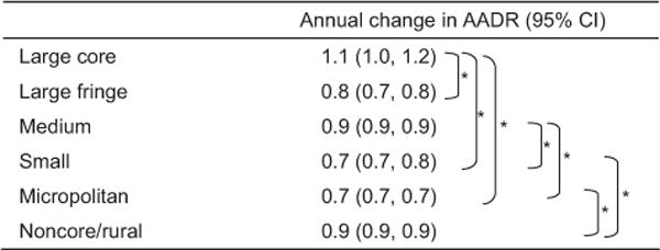
Annual change in age-adjusted death rate due to drug poisoning by urban/rural status
*Significant differences between groups, adjusted for multiple comparisons using Scheffe’s test
AADR, age-adjusted death rate
Figure 2.
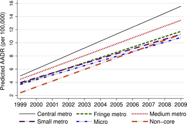
Age-adjusted death rates due to drug poisoning in the U.S. by level of urbanization, 1999–2009
Similar time trends by region of the country can be seen in Figure 3. Estimated drug-poisoning AADRs were roughly similar in 1999 across most regions of the country (with the exception of the West North Central, which had very low drug-poisoning AADRs throughout the study period). Over time, estimated rates diverged, with the highest AADRs in 2009 observed for the Pacific, Mountain, and East South Central regions and the lowest observed for the West North Central.
Figure 3.
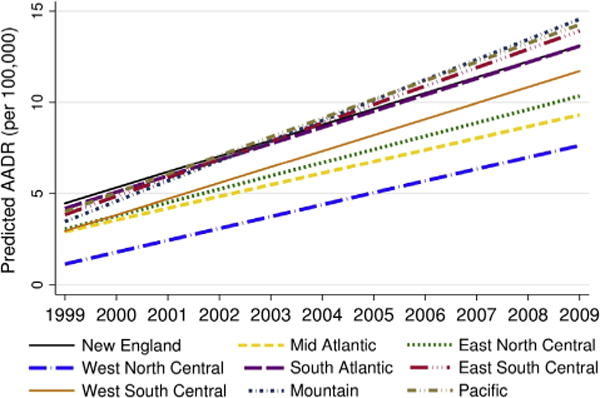
Age-adjusted death rates due to drug poisoning in the U.S. by region of the country, 1999–2009
Figure 4 illustrates the geographic patterns in drug-poisoning mortality over time (annual estimates for 1999–2009 can be seen in Appendix B, available online at www.ajpmonline.org). In 1999–2000, the vast majority of counties (72%) had estimated drug-poisoning AADRs of less than five per 100,000 per year. Only 3% had estimated AADRs of ten or more per 100,000 per year. By 2008–2009, only 10% of counties had estimated drug-poisoning AADRs less than five per 100,000 per year, and 54% of counties had estimated AADRs of ten or more per 100,000 per year.
Figure 4.
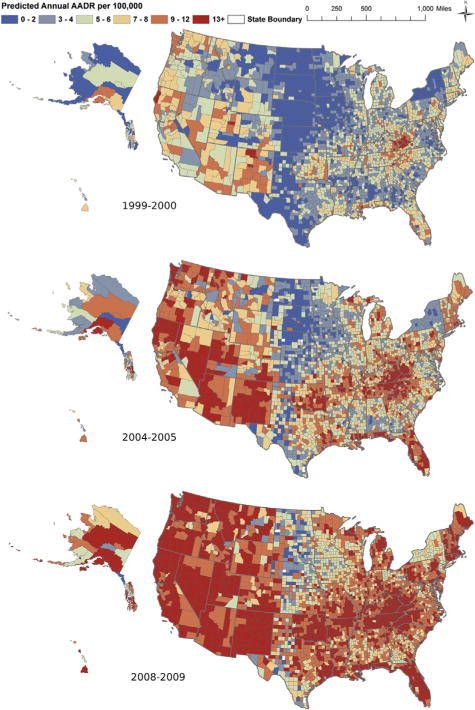
Maps of predicted age-adjusted death rates due to drug poisoning (per 100,000), 1999–2000, 2004–2005, 2008–2009
Model Fit and Evaluation
Table 1 describes the results of the two-stage models. Overall, the fully adjusted models explained approximately 75% of the county-level variance in probability of observing zero deaths, and the ICC was reduced from 0.7 to 0.3. In Stage-2 models, approximately 49% of the between-county variance in AADR was explained by the covariates included, and the ICC decreased from 0.4 to 0.3. Approximately 26% of the within-county variance in log-AADR was explained by the included covariates.
Table 1.
Variance and model diagnostics from Stage 1 and 2 null and adjusted models
| Model diagnostics | Stage 1: probability of zero deaths | Stage 2: log-transformed AADR | ||
|---|---|---|---|---|
| Null | Adjusted | Adjusted | Adjusted | |
| Random effectsa | ||||
| Level-1 variance | – | – | 0.3 | 0.3 |
| Level-2 variance | 6.2 | 0.3 | 0.2 | 0.1 |
| Fit statistics | ||||
| −2 log-likelihood | 31394.2 | 26623.4 | 47276.2 | 39288.9 |
| AIC | 31398.2 | 26665.4 | 47282.2 | 39344.9 |
| BIC | 31415.1 | 26842.9 | 47306.4 | 39571.1 |
| ICC | 0.7 | 0.3 | 0.4 | 0.3 |
| PCV Level 1 | – | – | – | 26% |
| PCV Level 2 | – | 75% | – | 49% |
Level-1 variance refers to the within-county variance in log-AADR (due to within-county variation over time); Level-2 variance refers to the between-county variance in probability of observing no deaths or the log-AADR. GLLAMM does not calculate within-county variance for logistic models.
AADR, age-adjusted death rate; AIC, Akaike’s information criterion; BIC, Bayesian information criterion; ICC, intraclass correlation coefficient; PCV, proportion change in variance
Although the residuals from each individual stage of the models did not display any obvious violations of assumptions, the overall “quasi-residual” differences between actual AADR and predicted AADR were correlated highly with actual AADR (r2 =0.74). In other words, the final estimated AADR produced by the two-stage modeling procedure resulted in underestimates of AADRs in areas where actual AADRs were very high. One consequence of this is that the overall quasi-residuals were much larger and more variable for rural counties (Appendix C, available online at www.ajpmon line.org).
Rural counties, on average, had very low probabilities of observing a death but some of the highest death rates due to drug poisoning. When looking only at counties that recorded a death for a given year (i.e., Stage 2 of the modeling procedure), the drug-poisoning AADRs were higher for rural areas compared to all other categories of urbanization, although rates increased at a similar pace from 1999–2009 for both rural areas and central cities (Figure 5).
Figure 5.
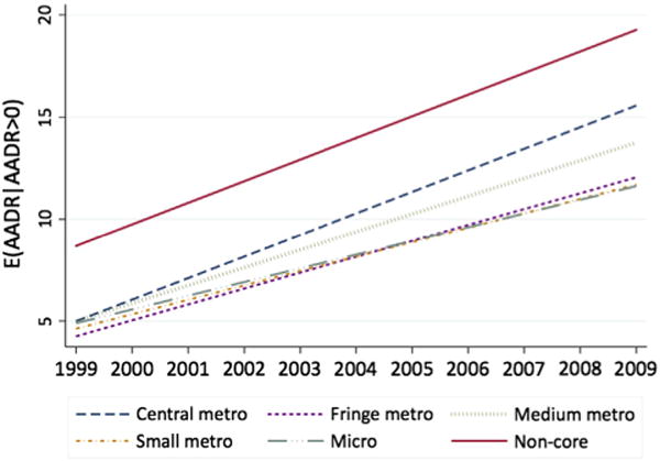
Age-adjusted death rates due to drug poisoning, given that a death was observed, by level of urbanization, 1999–2009
Discussion
Drug-poisoning fatalities have increased by more than 300% across the U.S. over the past 10 years. Although only 3% of counties had drug-poisoning AADRs of more than ten per 100,000 per year in 1999–2000, 54% had annual AADRs of more than ten per 100,000 in 2008–2009. There was substantial geographic variation in drug-poisoning mortality and increases over time. For example, drug-poisoning AADRs were lowest in the West North Central area of the U.S. throughout the study period. Although the Pacific, Mountain, and East South Central areas of the U.S. had drug-poisoning AADRs that were similar to those in other areas of the country in 1999, poisoning mortality increased rapidly in these regions over time; the highest AADRs were observed in these areas in 2009. Maps of drug-poisoning mortality over time illustrated that AADRs greater than 29 per 100,000 per year were largely concentrated to Appalachian counties in 1999–2000; by 2008–2009, counties across the entire U.S. displayed AADRs of more than 29 per 100,000 per year. These high rates could be seen in Alaska, Hawaii, the entire Pacific region, New Mexico, Oklahoma, Appalachia, the southern coasts of Louisiana and Mississippi, Florida, and New England.
Increases in drug-poisoning AADRs were larger in rural areas, where drug-poisoning death rates grew by 394% as compared to 279% for large central metropolitan counties. These findings are consistent with previous research looking at poisoning mortality due to narcotics from 1999 to 20049 and suggest that this pattern has continued through 2009. Although the urbanization by time interaction was significant and results suggest that AADRs increased to a larger degree in rural areas, drug-poisoning mortality was higher for central urban areas compared to rural areas across the study period. The interaction suggests that both central metropolitan and rural areas experienced similar absolute rates of increase (i.e., slopes) in drug-poisoning AADRs from 1999 to 2009; and that these rates of increase were more rapid than those seen in fringe or small metropolitan or micropolitan areas. However, because the AADRs in rural areas were substantially lower in 1999 as compared to central cities, the percentage increase was larger for rural areas over time (394%) compared to urban (279%).
A few, but not all, studies have reported similar patterns. For example, one study44 of West Virginia reported more rapid increases in drug-poisoning fatalities in rural areas compared to metropolitan areas, whereas another study45 reported no differences in mortality by population density. Another study in Oklahoma also reported larger increases in overdose death rates from 1997 to 2006 in rural areas as compared to urban areas.46 Other larger studies utilizing national vital statistics have reported similar findings to those presented here, whereby larger increases in drug-poisoning mortality were evidenced by rural areas as compared to larger metropolitan cities.9
There are several factors that could contribute to inconsistent findings with respect to urban–rural differences in drug-poisoning mortality. First, urban–rural classification could be serving as a proxy for geographic variation, particularly in studies that examine limited geographic areas. As the maps show, there is a large concentration of extremely high drug-poisoning fatalities in Appalachia, which encompasses rural areas across several states, whereas rural areas in other states such as North and South Dakota or New York have very low rates. Second, previous studies have not used small-area estimation techniques to examine drug-poisoning mortality by county or two-stage modeling procedures to account for the zero-inflated and right-skewed distribution of AADRs. Therefore, it is unclear whether previous findings may have been a consequence of unstable rate estimation in areas with small populations or the result of an underlying pattern where rural areas exhibit higher drug-poisoning mortality and more rapid increases over time (or both).
Given that a death occurred, the AADRs in rural areas were higher than those observed for more metropolitan areas. However, most rural counties in the U.S. had very low predicted probabilities of having a death; 88% of the zero deaths observed for a given county in a given year occurred in rural counties. Subsequently, the two-stage modeling procedure that combined the probability of observing a death with the estimated death rate reduced extreme AADRs in areas with low probabilities (i.e., rural counties). This is exactly the purpose of using small-area estimation techniques, as these procedures generate stable rates by borrowing information across counties and shrinking extreme values; but there is a tradeoff between improving the stability of rates and accurately capturing extreme values.
The small-area estimation technique utilized did not account for spatial dependence in generating county-level estimates. In other words, the modeling approach utilized information from counties with similar characteristics to shrink extreme values toward the mean. However, information about the proximity of counties was not used to inform these estimates. Alternative strategies that account for potential spatial dependencies by shrinking estimates toward local means,47,48 or hierarchical Bayes,49–52 could be explored in future studies in this area. However, Datta and Ghosh53 have noted that small-area estimates are typically robust to the frequentist or Bayesian method of estimation.
There are a few additional limitations of this analysis worth noting. Poisoning deaths, which often require lengthy investigations, are typically among the causes that remain pending at the close of the file. Although the percentage of pending cases at the state level was included as a covariate, it is possible that drug-poisoning deaths were underestimated, and it is unknown whether these underestimates may vary by county and year in a systematic way.54 Additionally, examination of the quasi-residuals—the difference between actual AADRs and the predicted—highlighted that predicted AADRs underestimated drug-poisoning AADRs in areas where rates were extremely high. Future research is needed to determine whether this underestimation is a result of the two-stage modeling and small-area estimation methods, residual spatial variation, or omitted variables such as physician prescribing patterns of narcotics by county or prevalence of doctor-shopping and drug-diversion.4
Supplementary Material
Acknowledgments
The findings and conclusions in this paper are those of the author(s) and do not necessarily represent the official position of the National Center for Health Statistics, CDC.
Appendix: Supplementary data
Supplementary data associated with this article can be found, in the online version, at http://dx.doi.org/10.1016/j.amepre.2013.07.012.
Footnotes
No financial disclosures were reported by the authors of this paper.
References
- 1.Warner M, Chen LH, Makuc DM, Anderson RN, Minino AM. Drug poisoning deaths in the U.S., 1980–2008. NCHS Data Brief. 2011:1–8. [PubMed] [Google Scholar]
- 2.CDC. Vital signs: overdoses of prescription opioid pain relievers—U.S, 1999–2008. MMWR Morb Mortal Wkly Rep. 2011;60:1487–92. [PubMed] [Google Scholar]
- 3.Substance Abuse and Mental Health Services Administration. The NSDUH Report: trends in nonmedical use of prescription pain relievers: 2002 to 2007. Rockville MD: 2009. [Google Scholar]
- 4.Paulozzi LJ, Ryan GW. Opioid analgesics and rates of fatal drug poisoning in the U.S. Am J Prev Med. 2006;31:506–11. doi: 10.1016/j.amepre.2006.08.017. [DOI] [PubMed] [Google Scholar]
- 5.Frosch D. Prescription drug overdoses plague. New Mexico: New York Times; 2012. Jun 8, [Google Scholar]
- 6.Hiaasen S. Pain pills from South Florida flood Appalachian states. Miami Herald. 2009 Apr 8; [Google Scholar]
- 7.CDC. CDC grand rounds: prescription drug overdoses—a U.S. epidemic. MMWR Morb Mortal Wkly Rep. 2012;61:10–3. [PubMed] [Google Scholar]
- 8.McDonald DC, Carlson K, Izrael D. Geographic variation in opioid prescribing in the U.S. J Pain. 2012;13(10):988–96. doi: 10.1016/j.jpain.2012.07.007. [DOI] [PMC free article] [PubMed] [Google Scholar]
- 9.Paulozzi LJ, Xi Y. Recent changes in drug poisoning mortality in the U.S. by urban-rural status and by drug type. Pharmacoepidemiol Drug Saf. 2008;17:997–1005. doi: 10.1002/pds.1626. [DOI] [PubMed] [Google Scholar]
- 10.CDC. Community-based opioid overdose prevention programs providing naloxone—U.S., 2010. MMWR Morb Mortal Wkly Rep. 2012;61(6):101–5. [PMC free article] [PubMed] [Google Scholar]
- 11.CDC. Vital signs: risk for overdose from methadone used for pain relief —U.S., 1999–2010. MMWR Morb Mortal Wkly Rep. 2012;61(26):493–7. [PubMed] [Google Scholar]
- 12.Chakravarthy B, Shah S, Lotfipour S. Prescription drug monitoring programs and other interventions to combat prescription opioid abuse. West J Emerg Med. 2012;13(5):422–5. doi: 10.5811/westjem.2012.7.12936. [DOI] [PMC free article] [PubMed] [Google Scholar]
- 13.Minino AM, Murphy SL, Xu J, Kochanek KD. Deaths: final data for 2008. Natl Vital Stat Rep. 2011;59:1–126. [PubMed] [Google Scholar]
- 14.Heron M, Hoyert DL, Murphy SL, Xu J, Kochanek KD, Tejada-Vera B. Deaths: final data for 2006. Natl Vital Stat Rep. 2009;57:1–134. [PubMed] [Google Scholar]
- 15.Minino AM, Heron MP, Murphy SL, Kochanek KD. Deaths: final data for 2004. Natl Vital Stat Rep. 2007;55:1–119. [PubMed] [Google Scholar]
- 16.Kochanek KD, Murphy SL, Anderson RN, Scott C. Deaths: final data for 2002. Natl Vital Stat Rep. 2004;53:1–115. [PubMed] [Google Scholar]
- 17.Arias E, Anderson RN, Kung HC, Murphy SL, Kochanek KD. Deaths: final data for 2001. Natl Vital Stat Rep. 2003;52:1–115. [PubMed] [Google Scholar]
- 18.Minino AM, Arias E, Kochanek KD, Murphy SL, Smith BL. Deaths: final data for 2000. Natl Vital Stat Rep. 2002;50:1–119. [PubMed] [Google Scholar]
- 19.Hoyert DL, Arias E, Smith BL, Murphy SL, Kochanek KD. Deaths: final data for 1999. Natl Vital Stat Rep. 2001;49:1–113. [PubMed] [Google Scholar]
- 20.Minino AM, Anderson RN, Fingerhut LA, Boudreault MA, Warner M. Deaths: injuries, 2002. Natl Vital Stat Rep. 2006;54:1–124. [PubMed] [Google Scholar]
- 21.DHHS, Health Resources and Services Administration. Area resource file (ARF) 2000 [Google Scholar]
- 22.Federal Bureau of Investigation. Uniform crime reports. 2000 [Google Scholar]
- 23.U.S. Departmentof of Commerce, Bureau of the Census. Census of population and housing, 2000: Summary File 3. 2002 [Google Scholar]
- 24.Ingram DD, Franco SJ. NCHS urban-rural classification scheme for counties. Vital Health Stat. 2012;2(154):1–65. [PubMed] [Google Scholar]
- 25.Warner M, Chen LH. Variations in the reporting of national data for drug poisoning mortality. National Vital Statistics system, 1999–2009; Presentation at the Council of State and Territorial Epidemiologists Conference; 2012 Jun 3–7; Omaha NE. [Google Scholar]
- 26.Everitt B, Hothorn T. Principal components analysis. In: Everitt B, Hothorn T, editors. An introduction to applied multivariate analysis with R. New York NY: Springer; 2011. pp. 61–103. [Google Scholar]
- 27.Zhang F, Huang CL, Lin BH, Epperson JE. Modeling fresh organic produce consumption with scanner data: a generalized double hurdle model approach. Agribusiness. 2008;24:510–22. [Google Scholar]
- 28.Bilgic A, Florkowski WJ. Application of a hurdle negative binomial count data model to demand for bass fishing in the southeastern U.S. J Environ Manage. 2007;83:478–90. doi: 10.1016/j.jenvman.2006.10.009. [DOI] [PubMed] [Google Scholar]
- 29.Baughman AL. Mixture model framework facilitates understanding of zero-inflated and hurdle models for count data. J Biopharm Stat. 2007;17:943–6. doi: 10.1080/10543400701514098. [DOI] [PubMed] [Google Scholar]
- 30.Labeaga JM. A double-hurdle rational addiction model with heterogeneity: estimating the demand for tobacco. J Econom. 1999;93:49–72. [Google Scholar]
- 31.Yen ST, Jensen HH, Wang QB. Cholesterol information and egg consumption in the U.S.: a nonnormal and heteroscedastic double-hurdle model. Eur Rev Agric Econ. 1996;23:343–56. [Google Scholar]
- 32.Kowalski KG, McFadyen L, Hutmacher MM, Frame B, Miller R. A two-part mixture model for longitudinal adverse event severity data. J Pharmacokinet Phar. 2003;30:315–36. doi: 10.1023/b:jopa.0000008157.26321.3c. [DOI] [PubMed] [Google Scholar]
- 33.Alfo M, Maruotti A. Two-part regression models for longitudinal zero-inflated count data. Can J Stat. 2010;38:197–216. [Google Scholar]
- 34.Wang LJ. IRT-ZIP Modeling for multivariate zero-inflated count data. J Educ Behav Stat. 2010;35:671–92. [Google Scholar]
- 35.Xie H, McHugo G, Sengupta A, Clark R, Drake R. A method for analyzing longitudinal outcomes with many zeros. Ment Health Serv Res. 2004;6:239–46. doi: 10.1023/b:mhsr.0000044749.39484.1b. [DOI] [PubMed] [Google Scholar]
- 36.Hall DB, Zhang ZG. Marginal models for zero inflated clustered data. Stat Model. 2004;4:161–80. [Google Scholar]
- 37.Li N, Elashoff DA, Robbins WA, Xun L. A hierarchical zero-inflated log-normal model for skewed responses. Stat Methods Med Res. 2011;20:175–89. doi: 10.1177/0962280208097372. [DOI] [PubMed] [Google Scholar]
- 38.Afifi AA, Kotlerman JB, Ettner SL, Cowan M. Methods for improving regression analysis for skewed continuous or counted responses. Annu Rev Public Health. 2007;28:95–111. doi: 10.1146/annurev.publhealth.28.082206.094100. [DOI] [PubMed] [Google Scholar]
- 39.Rao JNK. Small area estimation. Hoboken NJ: Wiley; 2003. [Google Scholar]
- 40.Skrondal A, Rabe-Hesketh S. Prediction in multilevel generalized linear models. J R Stat Soc Stat. 2009;172:659–87. [Google Scholar]
- 41.Rabe-Hesketh S, Skrondal A, Pickles A. Maximum likelihood estimation of limited and discrete dependent variable models with nested random effects. J Econom. 2005;128:301–23. [Google Scholar]
- 42.ESRI. ArcGIS desktop: release 10. Redlands CA: Environmental Systems Research Institute; 2011. [Google Scholar]
- 43.Bender R, Lange S. Adjusting for multiple testing—when and how? J Clin Epidemiol. 2001;54(4):343–9. doi: 10.1016/s0895-4356(00)00314-0. [DOI] [PubMed] [Google Scholar]
- 44.Wunsch MJ, Nakamoto K, Behonick G, Massello W. Opioid deaths in rural Virginia: a description of the high prevalence of accidental fatalities involving prescribed medications. Am J Addict. 2009;18:5–14. doi: 10.1080/10550490802544938. [DOI] [PMC free article] [PubMed] [Google Scholar]
- 45.Hall AJ, Logan JE, Toblin RL, et al. Patterns of abuse among unintentional pharmaceutical overdose fatalities. JAMA. 2008;300:2613–20. doi: 10.1001/jama.2008.802. [DOI] [PubMed] [Google Scholar]
- 46.Piercefield E, Archer P, Kemp P, Mallonee S. Increase in unintentional medication overdose deaths: Oklahoma, 1994–2006. Am J Prev Med. 2010;39(4):357–63. doi: 10.1016/j.amepre.2010.05.016. [DOI] [PubMed] [Google Scholar]
- 47.Lawson AB. Bayesian disease mapping: hierarchical modeling in spatial epidemiology. Boca Raton FL: Taylor & Francis Group; 2009. [Google Scholar]
- 48.Lawson AB, Song HR, Cai B, Hossain MM, Huang K. Space-time latent component modeling of geo-referenced health data. Stat Med. 2010;29(19):2012–27. doi: 10.1002/sim.3917. [DOI] [PMC free article] [PubMed] [Google Scholar]
- 49.Malec D, Davis W, Cao X. Small area estimates of overweight prevalence using the third national health and nutrition examination survey (NHANES III) Proc Am Stat Assoc. 1996;1:326–31. [Google Scholar]
- 50.Malec D, Davis WW, Cao X. Model-based small area estimates of overweight prevalence using sample selection adjustment. Stat Med. 1999;18(23):3189–200. doi: 10.1002/(sici)1097-0258(19991215)18:23<3189::aid-sim309>3.0.co;2-c. [DOI] [PubMed] [Google Scholar]
- 51.Malec D, Sedransk J, Moriarity CL, LeClere FB. Small area inference for binary variables in the National Health Interview Survey. J Am Stat Assoc. 1997;92(439):815–26. [Google Scholar]
- 52.Nandram B, Sedransk J, Pickle LW. Bayesian analysis and mapping of mortality rates for chronic obstructive pulmonary disease. J Am Stat Assoc. 2000;95(452):1110–8. [Google Scholar]
- 53.Datta G, Ghosh M. Small area shrinkage estimation. Stat Sci. 2012;27(1):95–114. [Google Scholar]
- 54.Landen MG, Castle S, Nolte KB, et al. Methodological issues in the surveillance of poisoning, illicit drug overdose, and heroin overdose deaths in New Mexico. Am J Epidemiol. 2003;157:273–8. doi: 10.1093/aje/kwf196. [DOI] [PubMed] [Google Scholar]
Associated Data
This section collects any data citations, data availability statements, or supplementary materials included in this article.