Relating multi-sequence longitudinal intensity profiles and clinical covariates in incident multiple sclerosis lesions

Abstract

The formation of multiple sclerosis (MS) lesions is a complex process involving inflammation, tissue damage, and tissue repair — all of which are visible on structural magnetic resonance imaging (MRI) and potentially modifiable by pharmacological therapy. In this paper, we introduce two statistical models for relating voxel-level, longitudinal, multi-sequence structural MRI intensities within MS lesions to clinical information and therapeutic interventions: (1) a principal component analysis (PCA) and regression model and (2) function-on-scalar regression models. To do so, we first characterize the post-lesion incidence repair process on longitudinal, multi-sequence structural MRI from 34 MS patients as voxel-level intensity profiles. For the PCA regression model, we perform PCA on the intensity profiles to develop a voxel-level biomarker for identifying slow and persistent, long-term intensity changes within lesion tissue voxels. The proposed biomarker's ability to identify such effects is validated by two experienced clinicians (a neuroradiologist and a neurologist). On a scale of 1 to 4, with 4 being the highest quality, the neuroradiologist gave the score on the first PC a median quality rating of 4 (95% CI: [4,4]), and the neurologist gave the score a median rating of 3 (95% CI: [3,3]). We then relate the biomarker to the clinical information in a mixed model framework. Treatment with disease-modifying therapies (p < 0.01), steroids (p < 0.01), and being closer to the boundary of abnormal signal intensity (p < 0.01) are all associated with return of a voxel to an intensity value closer to that of normal-appearing tissue. The function-on-scalar regression model allows for assessment of the post-incidence time points at which the covariates are associated with the profiles. In the function-on-scalar regression, both age and distance to the boundary were found to have a statistically significant association with the lesion intensities at some time point. The two models presented in this article show promise for understanding the mechanisms of tissue damage in MS and for evaluating the impact of treatments for the disease in clinical trials.

Highlights

• •Pipeline to extract voxel level longitudinal profiles from four MRI sequences within lesion tissue
• •Propose two statistical models to relate clinical covariates to the longitudinal profiles
• •Develop a biomarker that identifies areas of slow, long-term intensity changes at a voxel level
• •We validate the biomarker with ratings by two expert MS clinicians

1. Introduction

Structural magnetic resonance imaging (MRI) can be used to detect lesions in the brains of multiple sclerosis (MS) patients. The formation of these lesions is a complex process involving inflammation, tissue damage, and repair — all of which MRI has been shown to be sensitive. The McDonald criteria for diagnosis of MS emphasize the key role of dissemination of lesions in the central nervous system on MRI not only in space, but also in time (Polman et al., 2011). Characterizing the longitudinal behavior of lesions on structural MRI is therefore likely to be important for monitoring disease progression and response to therapy and for understanding the etiology of the disease. Surprisingly, there is poor association between clinical findings and the radiological extent of involvement on MRI using traditional volumetric measures, a phenomenon referred to as the clinico-radiological paradox (Barkhof, 2002). Here we address this paradox by modeling the association between the longitudinal behavior of lesions after incidence on MRI and clinical covariates and disease-modifying treatment.

Previous work to characterize the longitudinal behavior of lesions on structural MRI and to further relate these changes to clinical information has only involved single structural MRI sequences. In the work of Meier and Guttmann (2003), Meier and Guttmann (2006) and Meier et al. (2007), longitudinal lesion behavior is characterized only on the intensity normalized proton density (PD) volume, using bi-weekly MRI studies. Although they did not relate these changes to clinical covariates, it was found that the maximal insult within a lesion occurred at the center of the lesion, that lower initial intensity within a lesion was predictive of repair, and that most lesion activity did not last beyond 10 weeks. More recently, Ghassemi et al. (2014) examined the change over a 2-year period in normalized T1-weighted (T1) intensity within new lesions, and compared these changes in pediatric and adult-onset MS patients. A generalized linear mixed-effects model was used to relate clinical covariates, such as disease duration and treatments, to changes in intensity in the MRI. The only statistically significant relationship was that the T1 intensity in lesions increased between incidence and 1-year follow-up, and this recovery was more pronounced in children. Work has also been done to relate longitudinal changes in lesion intensity to sample size calculations for clinical trials. Reich et al. (2015) used the change in the 25th percentile of intensity-normalized PD signal within a lesion over time to estimate necessary sample sizes for clinical trials of differing lengths. The 25th, 50th, and 75th percentiles of multiple MRI sequences were assessed, and it was found that the 25th percentile of the normalized PD yielded the smallest sample size requirements. A limitation of these studies is that each uses only one MRI sequence to characterize the behavior of the lesions, which ignores information known to be available in the other sequences (McFarland et al., 2002).

Here, we describe two models to understand the relationship between clinical covariates and the longitudinal intensity profiles in lesion tissue from the T1, T2, T2-weighted fluid-attenuated inversion recovery (FLAIR), and PD sequences. The first is a principal component analysis (PCA) and regression model and the second consists of function-on-scalar regression models (Fan and Zhang, 2000). We use multi-sequence MRI studies acquired at the National Institute of Neurological Disease and Stroke (NINDS), with subjects being scanned on average once every 37 days (sd 52.3, range [13, 889]) yielding an average of 21 scans per subject (sd 8.0, range [10, 37]). In the PCA and regression model, we first reduce the data to a scalar, voxel-level biomarker for identifying slow and persistent, long-term intensity changes (which we will refer to from this point on as intensity changes for simplicity) within lesion tissue. The ability of the biomarker to identify these changes is then validated in an expert rater trial with two raters, a neuroradiologist and a neurologist. After this validation, we relate the biomarker to clinical information in a voxel-level mixed-effects regression framework. In the function-on-scalar regression, we directly relate the entire longitudinal trajectories from each sequence to the clinical covariates. This allows for assessment of how the clinical information relates to the intensity points at the post-lesion incidence time periods at which these associations occur, unlike in the PCA regression model.

2. Material and methods

In this section, we first describe the image acquisition and preprocessing, followed by the patient demographics. Next, we briefly describe the longitudinal lesion intensity profiles in the subsection Lesion Profiles, with a more complete description of the pipeline for extracting these profiles provided in Appendix A. We then introduce two models for studying the relationship between the lesion profiles and the clinical information in the subsections Principal Component Analysis and Regression and Function-on-Scalar Regressions. The subsection Principal Component Analysis and Regression also includes the expert rater trial of the voxel-level biomarker for identifying intensity changes within lesion tissue. All analysis, except for image preprocessing, was performed in the R environment (R Development Core Team, 2008) using the R package oro.nifti (Whitcher et al., 2011).

2.1. Image acquisition and preprocessing

Whole-brain 2D FLAIR, PD, T2, and 3D T1 volumes were acquired in a 1.5 Tesla (T) MRI scanner (Signa Excite HDxt; GE Healthcare, Milwaukee, Wisconsin) using the body coil for transmission. The 2D FLAIR, PD, and T2 volumes were acquired using fast-spin-echo sequences, and the 3D T1 volume was acquired using a gradient-echo sequence. The PD and T2 volumes were acquired as short and long echoes from the same sequence. The scanning parameters were clinically optimized for each acquired image.

For image preprocessing, we use Medical Image Processing Analysis and Visualization (http://mipav.cit.nih.gov) and the Java Image Science Toolkit (http://www.nitrc.org/projects/jist) (Lucas et al., 2010). We interpolate all images for each subject at each visit to a voxel size of 1 mm³ and rigidly co-register all volumes longitudinally and across sequences to the Montreal Neurological Institute standard space (Fonov et al., 2009). We remove extracerebral voxels using a skull-stripping procedure (Carass et al., 2007). We automatically segment the entire brain using the T1 and FLAIR images (Shiee et al., 2010) to produce a mask of normal-appearing white matter (NAWM), or white matter excluding lesions. After preprocessing, studies were manually quality controlled by a researcher with over four years experience with structural MRI (EMS). Studies with motion or other artifacts were removed.

2.2. Patient demographics

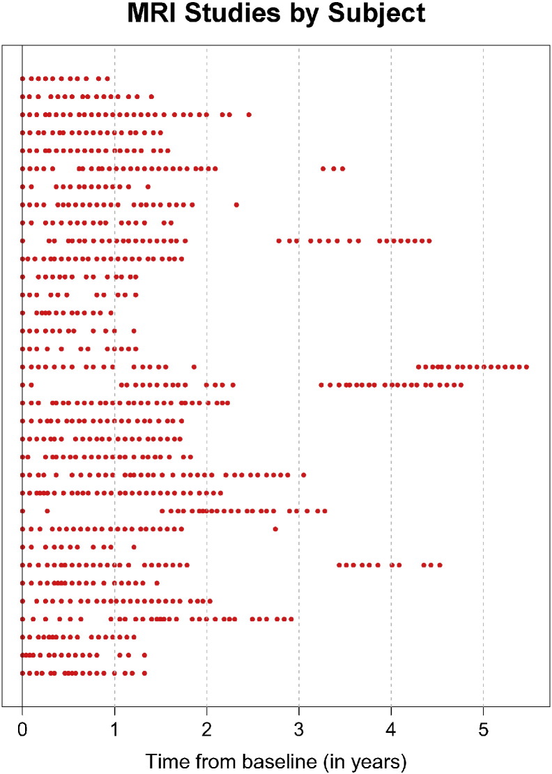
For this analysis, we use 60 subjects scanned at the NINDS, with the earliest scan performed in 2000 and the most recent scan performed in 2008. Three subjects were excluded during the expert validation because it was found that the longitudinal registration had failed, causing overall poor segmentation of lesion tissue. After exclusion of these subjects and subjects that did not have voxels with incident lesions that met a pre specified inclusion criteria (subjects scanned at least once within 40 days of lesion incidence and at least once 200 days after lesion incidence), there were 34 subjects left in the analysis. The 34 subjects included in the analysis had an average of 21 scans each (sd 8.0, range [10, 37]). Fig. 1 shows the time points at which each of the 34 subjects was scanned. Each row of the plot corresponds to a subject, and each point in the plot represents an MRI study, with time from the subject's baseline visit in years along the horizontal axis. The total follow-up time per subject was on average 2.2 years (sd 1.2, range [0.9, 5.5]). The mean age of the subjects at baseline was 37 years (sd 10.1, range [18,60]). At baseline, there were 30 subjects with relapsing–remitting MS (RRMS) and 4 subjects with secondary-progressive MS (SPMS). There were 20 females and 14 males, 14 subjects on disease-modifying treatment, and 2 subjects who received steroids at the baseline visit. The disease-modifying treatments and use of steroids for many of these subjects changed at subsequent follow-up visits.

Fig. 1.

The time points at which each of the 34 subjects included in the analysis was scanned. Each row of the plot is a subject, and each point in the plot represents an MRI study. The horizontal axis represents the time from the subject's baseline visit in years.

2.3. Lesion profiles

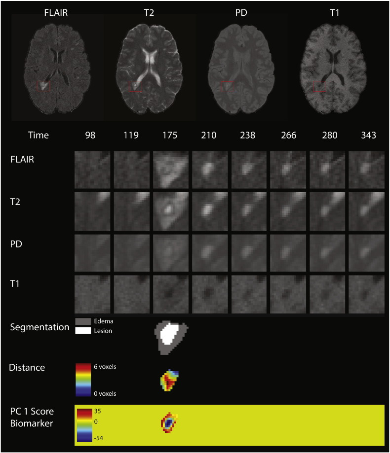
Fig. 2 shows an example of the longitudinal, multi-sequence MRI studies used for this analysis. For our analysis, we use intensity profiles from voxels that are detected during a subject's follow-up period. The first row of Fig. 2 shows the multiple MRI sequences at one time point (from left to right, the FLAIR, T2, PD, and T1 sequences). In each sequence, a red box shows an area with a lesion that develops during the follow-up period. The subsequent 4 rows of the figure show the longitudinal behavior within this red box. Each column of the figure shows a different MRI study, starting at 98 days after baseline in the far left column and going until 343 days after baseline. The lesion in the red box is first observed 175 days after baseline.

Fig. 2.

Longitudinal MRI studies within lesions. The first row of the figure shows an axial slice from the multiple MRI sequences, 175 days after baseline (from left to right, the FLAIR, T2, PD, and T1 sequences). In each sequence, a red box shows an area with a lesion that develops during the follow-up period. In the subsequent rows of the figure, we show the longitudinal behavior within this red box. Each column of the figure represents a different MRI study, starting at 98 days after baseline in the far left column and going until 343 days after baseline. A lesion is first identified in this area at 175 days. The first four rows show the longitudinal behavior of the FLAIR, T2, PD, and T1 sequences. The next row shows the segmentation of the edema and lesion tissue. The following row shows the distance to the boundary of abnormal MRI signal. The last row shows the score on the first PC, which identifies areas of lesion repair and permanent damage.

The pipeline for extracting the longitudinal voxel-level lesion profiles from the collection of multi-sequence structural MRI is divided into four steps: (1) identifying voxels with new lesion formation, (2) intensity normalization, (3) temporal alignment, and (4) temporal interpolation. We briefly describe these steps here and include an extended description of all steps in this pipeline in Appendix A. For the first step of identifying the lesion tissue, we distinguish between areas that contain vasogenic edema (which we will refer to simply as “edema”) and actual lesion tissue, which both manifest as areas of abnormal signal intensity, especially on the T2-weighted sequences. For this analysis, we are interested only in areas with tissue damage, as opposed to the neighboring edema. We combine two previously developed lesion segmentation methods, SuBLIME and OAISIS, to find new lesion voxels and distinguish between edema and lesion tissue (Sweeney et al., 2013a, Sweeney et al., 2013b). The row labeled “Segmentation” in Fig. 2 shows the edema and lesion tissue segmentation for each study at the time point in which the lesion was detected. The subsequent analysis is performed only on the lesion tissue in new lesion voxels.

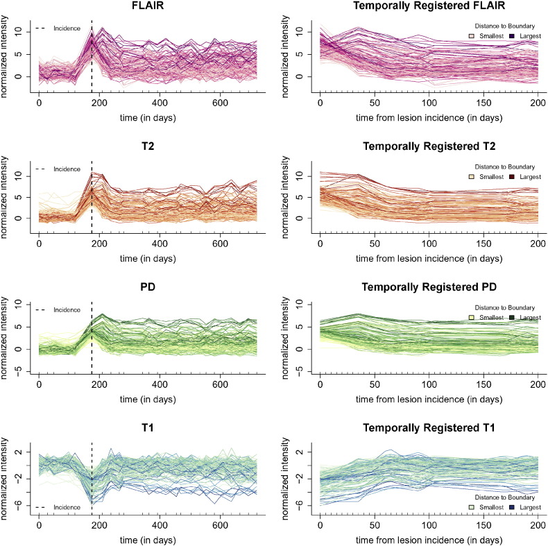
For intensity normalization, we put the units from each imaging sequence into standard deviations about the mean of intensities within the NAWM mask (Shiee et al., 2010) for the sequence, using the methodology of Shinohara et al. (2011) and Shinohara et al. (2014). After segmentation and normalization, the intensity normalized longitudinal profiles from the lesion in Fig. 2 for all four sequences can be seen in the first column of Fig. 3. From top to bottom in the first column of Fig. 3 we have the profiles from 150 randomly sampled voxels from the lesion in Fig. 2 for the FLAIR, T2, PD, and T1 sequences. Each line in the plot represents the longitudinal profile from a single voxel. The x-axis shows the time in days from the baseline visit, with the point of lesion incidence denoted by a vertical dashed line, and the y-axis shows the normalized sequence intensities.

Fig. 3.

Multi-sequence lesion profiles. The first column of the figure shows the full longitudinal profiles from all four sequences (from top to bottom, the FLAIR, T2, PD, and T1 sequences). The profiles are from 150 randomly sampled voxels from the lesion in Fig. 2, and for display purposes the periods between each study have been linearly interpolated. Each line in the plot represents the longitudinal profile from a single voxel. The x-axis shows the time in days from the subject's baseline visit, the time of lesion incidence is denoted by a dashed line, and the y-axis shows the normalized sequence intensities. The second column shows the same voxels after temporal alignment and linear interpolation over the 200 day period after incidence, the time period used in this analysis. The profiles are colored by distance to the boundary of abnormal MRI signal.

In this work, we are interested in the lesion dynamics only after lesion incidence, so we perform linear interpolation within the window after lesion incidence and up to 200 days post-incidence. We select the end point of 200 days, as it has been previously found that new T2 lesions show the most dramatic changes in intensity for three to four months (Meier et al., 2007), and we opt to be conservative and include some data beyond this reported stabilization point. Voxels are selected for the analysis if the subject has at least one visit 200 days or more after lesion incidence, and at least one visit within 40 days of incidence. Of the 60 subjects in this analysis, 34 have voxel profiles meeting this inclusion criteria, after removing the three subjects for poor longitudinal registration. We linearly interpolate over a grid of 0 to 200 days in increments of 5 days so that all profiles are observed on the same time grid. We denote the vector of observations from a voxel over this time grid for sequence S in voxel v for subject i in lesion l at registered study time t′ (since lesion incidence) as S_ilv^N(t′), for S = FLAIR, T1, T2, and PD. Then we let S_ilv^N be the longitudinal collection of these interpolated values, namely the 1 × 41 vector S_ilv^N = {S_ilv^N(t′) : t′ ∈ (0, 5, …, 200)}. The second column of Fig. 3 shows the temporally registered and linearly interpolated profiles, S_ilv^N, over the period of 0 to 200 days for the lesion in Fig. 2 for the same 150 randomly sampled voxels as shown in the first column.

2.4. Principal component analysis and regressions

In this section, we outline the PCA and regression modeling approach for studying the relationship between the longitudinal lesion profiles and demographics, disease, and treatment. We begin by describing the voxel-level biomarker for identifying intensity changes within lesion tissue. Next we describe the validation of this biomarker with an expert rater trial with two raters, a neuroradiologist and a neurologist. Last, we describe a mixed-model regression framework for relating the voxel-level biomarker to clinical covariates.

2.4.1. Biomarker

We begin by describing the voxel-level biomarker for identifying intensity changes within lesion tissue. The biomarker is the score on the first principal component (PC), after performing PCA on the longitudinal lesion profiles. To perform PCA on the longitudinal lesion profiles, we first concatenate the profiles for each voxel from the four sequences together. For each sequence and at each voxel, we have a 1 × 41 vector of longitudinal intensities, S_ilv^N. Let I_ilv denote the 1 × 164 dimensional vector of the four concatenated profiles, S_ilv^N, from subject i lesion l and voxel v. More precisely,

$$I_{ilv}=\left\{\mathit{FLAI}{R}_{ilv}^N,T{1}_{ilv}^N,T{2}_{ilv}^N,P{D}_{ilv}^N\right\}$$ (1)

and we index the entries I_ilv(j), where j = 1, …, 164 is the jth entry of the concatenated vector. Note that we first remove the mean from the concatenated profiles and then perform a PCA on these concatenated profiles. Let ϕ_k denote the kth PC, where ϕ_k is also indexed by j. The relationship between the score on the kth PC, the one-dimensional value ξ_ilv(k), and the observed trajectory for I_ilv(j) is:

$$I_{ilv}\left(j\right)={\displaystyle \sum _{k=1}^K{\xi }_{ilv}\left(k\right){\varphi }_k\left(j\right)\text{.}}$$ (2)

We focus on the first PC, ϕ₁, and the score on this component, ξ_ilv(1). The first PC is found to identify intensity changes at the voxel-level within lesions. Positive values of ξ_ilv(1) correspond to a return of the voxel to intensity values closer to that of normal-appearing tissue and negative values of ξ_ilv(1) correspond to the voxels maintaining intensity values closer to those at lesion incidence. This biomarker, ξ_ilv(1), collapses the full profiles at each voxel from the four sequences into a single scalar. We use the score on the first PC in this analysis, as the other PCs explain only 25% of the variation in the data, were not found to be associated with any biological processes, and are thus likely due to scanner-related and other noise. To assess the variability in both the mean and the first PC, we bootstrap this procedure by resampling subjects with replacement 1000 times (Efron and Tibshirani, 1994).

2.4.2. Expert validation of biomarker

We use expert validation to determine the quality of the lesion tissue segmentation (excluding edema) as well as the ability of the biomarker to identify areas of slow, long-term intensity change. For this validation we use two raters, a neuroradiologist with 11 years of research experience in MS (DSR) and a neurologist with 4 years of research experience in MS (MKS). For each lesion, we first determine the axial slice of the image that contains the largest number of voxels with abnormal signal intensity. Then for each lesion the two raters are presented the following: (1) the full axial slice for the FLAIR, T2, PD, and T1 volumes that contains the largest number of voxels with abnormal signal intensity; (2) the entire collection of longitudinal scans for a box containing the abnormal signal intensity in the FLAIR, T2, PD, and T1 volumes for this axial slice; (3) the segmentation of the lesion and edema tissue within this box; (4) the biomarker for the voxels segmented as lesion tissue within this box and a scale for the intensities within this image; (5) the entire collection of longitudinal scans for the FLAIR, T2, PD, and T1 weighted volumes within this box with the score for the first PC overlaid on the images for each scan after lesion incidence. The raters are then asked to rate the quality of the lesion tissue segmentation and the biomarker for identifying areas of intensity changes on an integer scale from 1 to 4, with each rating corresponding to the following: (1) failed miserably; (2) some redeeming features; (3) passed with minor errors; and (4) passed. Examples of the images presented to the raters for each lesion that received a rating of 1 through 4 for the score on the first PC by both raters are provided in Appendix A. Forty-seven lesions are selected at random to be repeated in the analysis to assess intra-rater reliability.

We report the median of the ratings of the lesion segmentation and the biomarker for each rater over all lesions. To assess between-rater and within-rater reliability, we report the Cohen's κ coefficients over all of the lesions and for the set of repeated lesions respectively, for both the rating of the biomarker and the lesion segmentation. We also report κ for the rating of the lesion segmentation and the biomarker for all lesions, for each rater, to determine if the quality of the segmentation and the quality of the biomarker are related. We nonparametrically bootstrap by subject with replacement 1000 times to produce the confidence intervals for the median of the ratings for each rater and the κ coefficients.

2.4.3. Regression model

The clinical information for each subject that we consider at each study visit consists of MS disease subtype, age, sex, an indicator of treatment with steroids, an indicator of disease-modifying treatment, and distance to the boundary of an area of abnormal signal intensity. An example of distance to the boundary of an area of abnormal signal intensity can be seen in the seventh row of Fig. 2. We center age at the mean age of 36 years over all of the voxel-level observations. During the observation period, many of the subjects were enrolled in clinical trials at NINDS to test various experimental therapies. Our indicator of disease-modifying treatment indicates treatment with any of the Food and Drug Administration-approved treatments, including interferon beta 1-a (intramuscular or subcutaneous), interferon beta 1-b, and glatiramer acetate, as well as experimental therapy. As many of the covariates change over time, we model the relationship between the lesion profiles and the value of the covariate at the time of lesion incidence for the particular profiles. For the following analysis, we have a total of 57,908 voxels from 315 lesions in 34 subjects.

We now introduce a linear mixed-effects model to relate the biomarker, that is the score on the first PC, to the clinical covariates (McCulloch and Neuhaus, 2001). We use the value of the covariate at the time of lesion incidence for the particular profiles, which can vary within subject. Thus, for added precision, the covariates that change over time are indexed by the subject index i, lesion index l and voxel index v, as voxels from the same lesion may have different times of incidence. For example, the sex of the subject does not change by time of lesion incidence, so it is only indexed by i. In contrast, age of the subject changes with voxel lesion incidence and is indexed by i, l and v. We also add random effects for subject and lesion, which we denote by b_i and b_l, respectively, with both following a normal distribution: b_i ~ N(0, σ_i²) and b_l ~ N(0, σ_l²), where σ² denotes the variance of the random effects. We consider the following basic model for the association between the biomarker, ξ_ilv(1), and the covariates:

$$\begin{array}{c}\hfill {\xi }_{ilv}\left(1\right)={\beta }_0+{\beta }_1{\mathrm{SPMS}}_{ilv}+{\beta }_2{\mathrm{Distance}}_{ilv}+{\beta }_3{\mathrm{Age}}_{ilv}+{\beta }_4{\left(\mathrm{Age}-4\right)}_{+ilv}\hfill \\ \hfill +{\beta }_5{\mathrm{Steroids}}_{ilv}+{\beta }_6{\mathrm{Male}}_i+{\beta }_7{\mathrm{Treatment}}_{ilv}+b_i+b_l+{\epsilon }_{ilv}\hfill \end{array}\text{.}$$

We assume that the error terms are independent and identically distributed, with each following a normal distribution, ε_ilv ~ N(0, σ_ϵ²). In the model, the term SPMS is an indicator of being diagnosed with SPMS where the comparison group is being diagnosed with RRMS. Note that the age term has been centered at the mean age of 36 years. The term (Age − 4)_+ ilv = Age_ilv ⋅ 1(Age_ilv > 4) is a spline term for centered age over 4 years (or age over 40 years), which was included in the model after visualizing the relationship between the biomarker and age. We also investigated simpler models with the same mixed-effects structure, but where we considered each covariate separately.

To test for associations, we use two procedures. First, we perform a parametric bootstrapping procedure (Efron and Tibshirani, 1994), and second we calculate p-values using a normal approximation for the distribution of the fixed-effects in the mixed-effects model (Barr et al., 2013). We use 1000 bootstrap samples for the bootstrap procedure. We perform the parametric bootstrap because steroid use and disease subtype of SPMS did not always appear in nonparametric bootstrap samples. A complete description of this procedure is found in Appendix A. We also use the normal approximation, as this approximation has been found to be a reasonable approximation for the distribution of the fixed-effects in most settings (Barr et al., 2013).

2.5. Function-on-scalar regressions

The previous model is an attempt to collapse the information from the four profiles (across sequences and time) into a single scalar at each voxel. As an alternative, we also fit a two-step function-on-scalar regression model (Fan and Zhang, 2000), where we can investigate the relationship between the covariates of interest and the profile at each time point. We fit a function-on-scalar regression model for each sequence separately. For simplicity of notation, we now use t for the registered time, as opposed to t′. The outcome in the model is the full lesion intensity profile:

$$\begin{array}{c}\hfill S_{ilv}^N\left(t\right)={\beta }_0^{\prime }\left(t\right)+{\beta }_1^{\prime }\left(t\right){\mathrm{SPMS}}_{ilv}+{\beta }_2^{\prime }\left(t\right){\mathrm{Distance}}_{ilv}+{\beta }_3^{\prime }\left(t\right){\mathrm{Age}}_{ilv}+{\beta }_4^{\prime }\left(t\right){\left(\mathrm{Age}-4\right)}_{+ilv}\hfill \\ \hfill +{\beta }_5^{\prime }\left(t\right){\mathrm{Steroids}}_{ilv}+{\beta }_6^{\prime }\left(t\right){\mathrm{Male}}_i+{\beta }_7^{\prime }\left(t\right){\mathrm{Treatment}}_{ilv}+{\mathrm{ϵ}}_{ilv}\left(t\right)\hfill \end{array}$$

for S = FLAIR, T1, T2, and PD. To fit the model, we use a two-step function-on-scalar regression implemented in the R package refund (Crainiceanu et al., 2014). The procedure first fits a scalar-on-scalar regression at each individual time point. Then the resulting coefficient functions are smoothed over time using a cubic spline basis with an automatically selected penalty on the second derivative.

To assess the variability in the coefficient functions and provide bootstrapped, point-wise 95% confidence intervals, we non-parametrically bootstrap by subject using 1000 resampled datasets. When samples do not contain subjects with a covariate, for example the indicator of steroids, we remove this sample from the bootstrap and replace it with another sample. The difference between the function-on-scalar regression and the PCA regression model is that PCA collapses the entire temporal intensity profile of the voxel into a scalar. By contrast, the function-on-scalar regression investigates the association at every time point. While function-on-scalar regression is more comprehensive and interpretable, it is more appropriate when there are strong functional effects that are not captured by a small number of principal components, due to the potential for decreased statistical power.

3. Results

3.1. Principal component analysis and regression

3.1.1. Biomarker

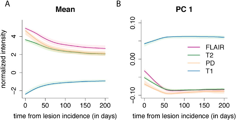
In Fig. 4A we show the mean profiles for each sequence over the registered 200 day period, and in Fig. 4B we show the first PC, ϕ₁, for each sequence over the registered 200 day period, where the first PC is divided into different sequences for purposes of presentation. The subfigures for both the mean and the first PC show the bootstrapped 95% confidence intervals. The first PC explains 75% (95% CI: [72%, 76%]) of the variation in the concatenated longitudinal profiles.

Fig. 4.

The mean profile and first PC for each of the four sequences. Panel A of the figure shows the mean profiles for each of the imaging sequences over the registered 200 day period, and panel B shows the first PC for each of the imaging sequences. The first PC explains 75% of the variation in the concatenated longitudinal profiles. Along the x-axis for both plots is plotted the time in days since lesion detection. The 95% confidence intervals in both panels are obtained using 1000 nonparametric bootstrapped samples.

To interpret the PCs, we recall that the normalization procedure puts the volumes into units of standard deviations above the mean of the NAWM. Therefore a value of 0 on the image corresponds to the average value of NAWM from the particular MRI scan. The mean profiles for the FLAIR, T2, and PD are all above 0 throughout the time course, as lesions are hyperintense on these sequences. In contrast, the mean profile for the T1 sequence is below 0, as lesions are hypointense on this sequence. The first PC for the FLAIR, T2, and PD is negative throughout the time course, with values closer to 0 at lesion incidence (time 0). Positive scores on this PC indicate a decrease in the signal in these sequences, which corresponds to a return of the voxel to intensity values closer to that of normal-appearing tissue. In contrast, negative scores indicate the voxel maintaining intensity values closer to those at lesion incidence, with more hypointensity than the average profile. Similarly, for T1 the first PC is positive throughout the time course, with values closer to 0 at lesion incidence. Positive scores on this PC indicate increased signal on the T1. As lesions are hypointense on the T1, this also indicates a return of the voxel to intensity values closer to that of normal-appearing tissue. Negative scores again correspond to the voxels maintaining intensity values closer to those at lesion incidence.

We therefore consider the score on the first PC to be a biomarker of intensity changes within the lesion at the voxel level. In the last row of Fig. 2 we see the PC scores or the biomarker from the lesion that is shown in the figure. We see that the positive scores indicate areas of the lesion that return to values of normal-appearing tissue, while the negative scores show areas that remain at the intensity values at lesion incidence.

3.1.2. Expert validation of biomarker

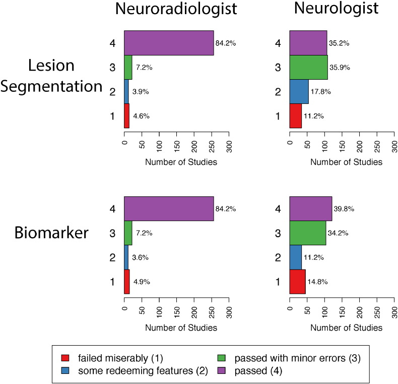
We use expert validation to determine the quality of the lesion segmentation (excluding edema tissue) and the ability of the biomarker to identify areas of slow, long-term intensity change. The distributions of the ratings for the two raters for both the lesion segmentation and the biomarker are shown in Fig. 5. The first row of plots in Fig. 5 shows the distribution of the ratings for the lesion segmentation and the second row shows the ratings for the biomarker. Plots in the left column are ratings by the neuroradiologist, and plots on the right column are ratings by the neurologist. The median rating for both the lesion segmentation and the biomarker by the neuroradiologist is 4 (95% CI: [4,4]), which is a rating of passed, the highest possible rating. The median rating for both the lesion segmentation and the biomarker by the neurologist are 3 (95% CI: [3,3]), which is a rating of passed with minor errors. Note that criteria for assigning scores were not discussed between the two raters prior to their respective analyses.

Fig. 5.

Distributions of the ratings for the two raters. The first row of plots shows the distributions of the ratings for the lesion segmentation, and the second row shows the ratings for the biomarker. Plots in the left column are ratings by the neuroradiologist, and plots on the right column are ratings by the neurologist. Each plot shows the number of studies that failed miserably (1), had some redeeming features (2), passed with minor errors (3), and passed (4) along with the percentage of each rating.

The κ coefficients for the within- and between-rater agreement for both the lesion segmentation and the scores on the biomarker are shown in Table 1. The values for the κ coefficient range between 0 and 1, with a value of 1 indicating total agreement and 0 indicating no agreement. The within-rater agreement for the lesion segmentation and the score on the biomarker are higher for the neuroradiologist than the neurologist. There is only modest agreement between the neuroradiologist and neurologist on both ratings, with a κ coefficient of 0.29 (95% CI: [0.18, 0.41]) for the lesion segmentation and 0.24 (95% CI: 0.11, 0.39) for the score on the biomarker. This is due, in part, to the fact that the neurologist spread ratings of the studies between 3 and 4, while the neuroradiologist gave more ratings of 4.

Table 1.

κ coefficients for the ratings of the lesion segmentation and the biomarker. The table on the left shows the κ coefficients for the lesion segmentation, and the table on the right shows the same for the biomarker. The between-rater agreement is reported using all lesions. The within-rater agreement is reported using only the forty-seven repeated lesions.

	Lesion Segmentation		Biomarker
Neuroradiologist	Neurologist	Neuroradiologist	Neurologist
Neuroradiologist	0.92; (0.76,0.99)	0.29; (0.18, 0.41)	0.92; (0.76, 0.99)	0.24; (0.11, 0.39)
Neurologist		0.75; (0.62, 0.86)		0.72; (0.51, 0.86)

The κ coefficient for the agreement between the rating of the lesion segmentation and the biomarker is 0.97 (95% CI: 0.93, 1.00) for the neuroradiologist and 0.68 (95% CI: 0.58, 0.78) for the neurologist. The high correlation between these ratings, especially for the neuroradiologist, indicates that the quality of the segmentation impacts the quality of the rating of the biomarker. Comments from the raters mirrored this finding, as many of the low scores for both the lesion segmentation and the biomarker were due to (1) missing the first time point of lesion incidence and segmenting it as new lesion at a later time point; (2) not segmenting the entire lesion; and (3) parts of the same lesion being segmented (unnecessarily) at different time points. As both the ratings for the lesion segmentation and the score on the biomarker were high, the quality of the lesion segmentation does not appear to be negatively impacting the method.

3.1.3. Regression model

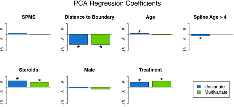
We fit both univariate and multivariate mixed-effects models to investigate the relationship between the covariates and the biomarker. The estimates of the coefficients from both models are shown in the bar plots in Fig. 6, with asterisks indicating statistical significance at the 5% level using the bootstrapped 95% confidence intervals. Tables containing the coefficient estimates, standard errors, t-statistics, p-values using the normal approximation, and 95% bootstrapped confidence intervals can be found in Appendix A for both the univariate and the multivariate models. There are no differences in the conclusions determined by the normal approximation and the bootstrapped 95% confidence intervals. For continuous covariates, such as age, the coefficient is interpreted as the expected change in the biomarker for a one unit increase in the covariate. For binary variables, such as disease subtype, the coefficient is interpreted as the difference in the expected change in the biomarker in the specified group. Therefore, positive coefficients are indicative of the voxel returning to intensity values closer to normal-appearing tissue with an increase in the covariate, while negative coefficients are indicative of the voxel maintaining the intensities at lesion incidence with an increase in the covariate (or in some rare cases having intensities that have an increasing departure from those of normal-appearing tissue over time with an increase in the covariate). The results indicate that voxels that are farther away from the boundary have increased risk for maintaining abnormal signal intensity. In this model, the coefficient for distance to the boundary has a value of − 9.4 (95% CI: [− 9.6, − 9.3]), indicating that for a one voxel (or 1 mm) increase in distance away from the boundary (toward the center of the lesion) the average value of the biomarker decreases by 9.4, adjusting for the other coefficients and the random effects. In the last row of Fig. 2, we see this spatial relationship between the biomarker and the distance to the lesion boundary, with positive scores near the boundary and negative scores near the center of the lesion. In both models, we found the use of disease-modifying treatment and steroids to be associated with return of a voxel to the value of normal-appearing tissue. The coefficient for treatment has a value of 5.4 (95% CI: [4.7, 6.1]), indicating that when subjects are on treatment the average value of the biomarker increases by 5.4, adjusting for the other coefficients and the random effects. The use of steroids has a similar interpretation, with a coefficient value of 4.3 (95% CI: [2.7, 5.9]).

Fig. 6.

Coefficients from the PCA Regression model. This figure shows bar plots of the coefficient estimates from the univariate and multivariate mixed-effects models with the biomarker as an outcome. The results from the univariate model are shown in blue, and the results from the multivariate model are shown in green. Asterisks indicate significance at the 5% level. In both the univariate and multivariate models, disease-modifying therapy, steroids, and age were found to be significant.

3.2. Function-on-scalar regression

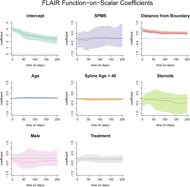
The resulting coefficient functions from the function-on-scalar regression with bootstrapped, point-wise 95% confidence intervals with the FLAIR profile as the outcome are shown in Fig. 7. Similar figures for models with the T2, PD, and T1 profiles are provided in Appendix A. The coefficient functions for continuous variables in the function-on-scalar regression model are interpreted as the change in the expected profile at each time point for a one unit increase in the covariate. Similarly, for binary variables, the coefficient function is interpreted as the change in the expected profile for the specified group. For the FLAIR profiles, the coefficient functions corresponding to distance to the boundary and age have bootstrapped 95% confidence intervals that do not overlap with 0 across any of the time points, and are therefore statistically significant at the .05 level. The coefficient function for distance to the boundary is greater than 0 throughout the entire trajectory, indicating that the farther away from the boundary the voxel is, the more the FLAIR hyperintensity is maintained within the voxel. For a one voxel (or 1 mm) increase in distance away from the boundary (toward the center of the lesion) the average normalized intensity of the trajectory increases by around 0.5 at all time points, adjusting for the other coefficients and the random effects. The result for distance from the boundary agrees with the results from the PCA regression model.

Fig. 7.

Coefficient functions from the function-on-scalar regression with the FLAIR profile as an outcome. Each dark line represents the coefficient function, and the shaded area represents a bootstrapped, point-wise 95% confidence interval. Along the x-axis of each plot is the time in days from lesion incidence. Along the y-axis is the value of the coefficient function at each time point. Only distance from the boundary and age were found to be different for 0 at any point along the profile.

4. Discussion

We introduce two models to relate clinical information to the longitudinal intensity profiles in lesion tissue from conventional MRI sequences. The first model is the PCA regression model, where we collapse the longitudinal, multi-sequence MRI information into a biomarker of slow, long-term intensity changes within the lesion at the voxel-level and then relate this to clinical information. We validate the ability of the biomarker to detect these intensity changes using an expert rater trial. The second model is the function-on-scalar regression model, which relates each longitudinal intensity profiles separately to the clinical information and allows for assessment of the time points in which the clinical information is impacting the profiles. The methodology presented here shows promise for both understanding the time course of tissue damage in MS and for evaluating the impact of neuroprotective or reparative treatments for the disease. The biomarker may be particularly useful in clinical trial settings, as it is sensitive to the effects of disease-modifying therapies and shows impressive performance in expert visual validation. Reliable methods to evaluate such treatments, which are currently under development, are lacking at present. In contrast to prior studies of change in lesion intensity in clinical trials, our work is focused on voxel-level analysis, and therefore it can provide spatial information about intensity recovery and does not artificially reduce the size of the data set. This may have implications on the sample size calculations for clinical trials. These methods are also broadly applicable to other imaging modalities and disease areas, in which longitudinal intensity profiles may lead to more sensitive and specific biomarkers.

In the PCA and regression model, we observe a statistically significant relationship between the biomarker and the use of disease-modifying therapy and steroids. Both treatment and steroids were associated with a return of a voxel to intensity values closer to that of normal-appearing tissue. The inference from both models in regard to disease-modifying treatment should only be taken as a proof-of-concept for the relationship between the imaging and the clinical covariates. The models may suffer from confounding by indication, which arises when individuals who are on a treatment are different from those who do not receive treatment, due to unobserved considerations. In the multivariate model, we adjust for age, sex, and disease subtype, but unobservable differences related to treatment choice may cause biased conclusions. However, bias in terms of treatment effect would most plausibly result in underestimation of improvements, as more aggressive therapies are commonly given to subjects with more aggressive or refractory disease. Thus, our findings might underestimate what would be observed in a randomized trial of disease-modifying therapy.

One limitation of this study was the relatively small number of subjects. Future work will involve deploying the methodology and models on a larger number of subjects (n = 34), in both observational studies and randomized clinical trials. While many of the coefficient functions from the function-on-scalar regression are not found to be statistically different from 0, this model may have more power with more subjects. For the bootstrap procedure we only have 34 subjects, resulting in wide confidence intervals for the estimated coefficient functions. In contrast, the regression using score outcomes identifies strong associations between specific covariates and multisequence longitudinal patterns of longitudinal intensities.

The two models presented in this work are fit voxel-wise and therefore may be sensitive to major misregistration within a study and between longitudinal studies for the same subject. The models are also sensitive to local displacement of tissue due to transient swelling in and around lesions or resorption of lesion tissue. We therefore do not call the slow changes in intensity within the voxels that are observed “tissue repair”, as we cannot be certain that the change is not due to misregistration or displacement of tissue from the lesions themselves. We do observe a relationship between the return of voxels to the intensity of normal-appearing tissue and both disease-modifying treatment and treatment with steroids, and therefore find this measure useful and deserving of further study. We also see an association with the distance to the boundary of the lesion and slow, long-term intensity changes — with voxels near the boundary of the lesion returning to baseline intensity and voxels near the center of the lesion maintaining abnormal signal intensity. Future work to assess tissue repair may involve investigating a nonlinear registration within individual lesions.

The methods described here use only conventional clinical imaging for patients with MS, namely FLAIR, T2, PD, and T1. While this is beneficial for using the methodology in a clinical trial setting or for analysis of retrospective imaging studies, one could also incorporate advanced imaging into the method. For example, magnetization transfer ratio imaging (Van Waesberghe et al., 1999), quantitative T1-weighted imaging (Filippi et al., 2000), and diffusion tensor imaging (Filippi et al., 2001) have been studied in MS lesions. The longitudinal dynamics of lesions on these images could be incorporated into our framework to better understand the behavior of lesions over time and the impact of disease-modifying therapies on this behavior.

For this analysis, all MRI studies are acquired on a single 1.5 T MRI scanner at one imaging center. Similar analysis could be performed at higher field strength, but for this analysis we use a 1.5 T dataset for the availability of the large retrospective cohort study over a long period of time. Although different scanning parameters were used for the acquisitions, further investigation is warranted into the robustness of the methods to changes in scanner, changes in magnetic field strength, as well changes in the imaging center.

Appendix A.

A.1. Longitudinal profile pipeline

Here we provide a more complete description of the procedure for extracting the longitudinal voxel-level lesion profiles, which is divided into four steps: (1) identifying voxels with new lesion formation, (2) intensity normalization, (3) temporal alignment, and (4) temporal interpolation. All voxels in this analysis are part of incident or enlarging lesions detected during the subject's follow-up period. All voxels that are part of lesions that existed at baseline are excluded from the analysis.

A.2. Identifying voxels with new lesion formation

When identifying voxels with new lesion formation, we distinguish between areas that contain vasogenic edema (which we will refer to simply as “edema”) and actual lesion, which both manifest as areas of abnormal signal intensity, especially on the T2-weighted sequences. For this analysis, we are interested in areas with tissue damage, as opposed to edema. To identify areas with new lesion formation, we first find areas in the MRI with new abnormal signal intensity, which includes both edema and lesion. We then segment lesions by analyzing subsequent visit data.

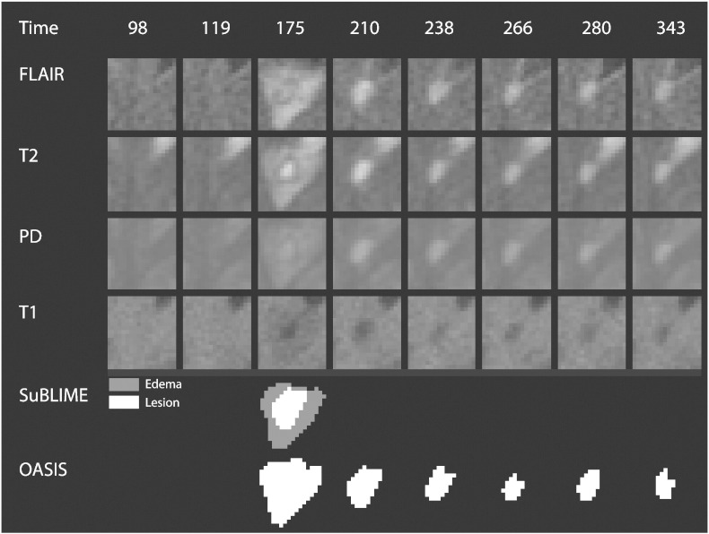
SuBLIME segmentation of voxel-level lesion incidence and enlargement is a method for detecting voxels that are part of an area of new abnormal signal intensity between two MRI studies (Sweeney et al., 2013a). For each subject, we produce SuBLIME maps between the respective sets of consecutive MRI studies. We exclude all abnormal signal intensity areas that contained fewer than 27 voxels, as these areas could be artifact or noise. We then produce cross-sectional lesion segmentations using OASIS segmentation of abnormal signal presence (Sweeney et al., 2013b). As the signal from edema disappears rapidly from the MRI after lesion formation, we locate the incident abnormal signal voxels using SuBLIME, but only include the voxels that are detected by OASIS at the following study visit, as these voxels should not contain edema. Therefore, only voxels that have an MRI study within 40 days after SuBLIME detects the area of abnormal signal intensity, where the intensity remains in the OASIS maps, are considered as lesion tissue and used in this analysis, as by this time edema would subside. We use expert validation by a neuroradiologist and a neurologist, both with experience in MS imaging, to confirm that this method is identifying lesion tissue, which we describe in detail in the subsection Expert Validation. The figure below shows the SuBLIME segmentation for each study and the OASIS segmentation for each study, corresponding to Fig. 2 from the paper. The row corresponding to the SuBLIME segmentation is further divided into edema and lesion voxels using the method described above. Only voxels that are part of lesion tissue are used in the analysis (Fig. 8).

Fig. 8.

SuBLIME and OASIS segmentations. Each column of the figure represents a different MRI study, starting at 98 days after baseline in the far left column and going until 343 days after baseline. A lesion is first identified in this area at 175 days. The first four rows show the longitudinal behavior of the FLAIR, T2, PD, and T1 sequences. The next rows show the SuBLIME segmentation of lesion incidence for each study and the OASIS segmentation of lesion presence in each study. The SuBLIME segmentation has been further divided into areas of edema and lesion.

A.3. Intensity normalization

Structural MRI is acquired in arbitrary units. Therefore, in addition to pulse sequence similarity, intensity normalization is paramount for comparing intensities in a voxel over time within subject and for comparing voxel intensities between subjects. We normalize each sequence separately on each scan by calculating the mean and standard deviation over a mask of the normal-appearing white matter (NAWM) from the brain segmentation described in the subsection Image Acquisition and Preprocessing (Shiee et al., 2010). We then subtract the mean from the intensity in each voxel and divide by the standard deviation (Shinohara et al., 2011, Shinohara et al., 2014). Let S_ilv(t) be the observed intensity from imaging sequence S in voxel v for subject i in lesion l at study time t, with S = FLAIR, T1, T2, and PD. Let μ_Si(t) and σ_Si(t) be the mean and standard deviation, respectively, over the NAWM mask for sequence S at scan time t for subject i. Then the normalized intensity in voxel v in lesion l for subject i at scan time t is:

$$S_{ilv}^N\left(t\right)=\frac{S_{ilv}\left(t\right)-{\mu }_{Si}\left(t\right)}{{\sigma }_{Si}\left(t\right)}\text{.}$$

Thus, all image intensities are expressed as a departure, in multiples of standard deviation of white matter intensities, from the subject's mean normal-appearing white matter (NAWM) in each imaging sequence.

A.4. Temporal alignment

The date of the study visit at which SuBLIME detects the lesion voxels is considered the time of incidence for this voxel. If a voxel is determined to be a new or enlarging lesion by SuBLIME more than once over the follow-up time, the first occurrence is considered to be the time of lesion incidence for that voxel. Voxel profiles from incident lesions during the follow-up of each subject are aligned in time, using the time of incidence as time 0, therefore any observations before incidence have a negative time and after lesion incidence have a positive time. Let t′ denote this aligned time scale. Then we have S_ilv^N(t′), where S_ilv^N(0) indicates the intensity in sequence S at the time of lesion incidence.

A.5. Temporal interpolation

Next we perform a temporal linear interpolation so that all voxels are observed on the same time grid. In this work, we are interested in the lesion dynamics only after lesion incidence, therefore we perform the linear interpolation within the window after lesion incidence and up to 200 days post-incidence. The end point of 200 days is selected as it has been previously found that new T2 lesions show the most dramatic changes in intensity for three to four months (Meier et al., 2007), and we opt to be conservative and include data beyond this reported stabilization point. Voxels are selected for the analysis if the subject has at least one visit 200 days or more after lesion incidence. Of the 60 subjects in this analysis, 34 have voxel profiles meeting this inclusion criteria, after removing the three subjects for poor longitudinal registration. We linearly interpolate over a grid of 0 to 200 days by increments of 5 days so that all profiles are observed on the same time grid. We denote the vector of observations from a voxel over this time grid for sequence S as S_ilv^N, where S_ilv^N is a 1 × 41 vector.

A.6. Parametric bootstrapping procedure

Let B be the number of bootstrap samples to be performed and let b index these B samples. Let Y_ilv be the outcome for an observation indexed by i, l, and v. Let X be the design matrix and β be the vector of the coefficients. For this analysis we have a model of the form:

$$Y_{ilv}=\mathit{X}\mathit{\beta }+b_i+b_l+{\epsilon }_{ilv}$$

where b_i ~ N(0, σ_i²) and b_l ~ N(0, σ_l²) are random intercepts, and ϵ_ilv ~ N(0, σ_ϵ²) is an error term. For the parametric model, we fit the above mixed-effect model to get an estimate of β, which we denote as $\widehat{\mathit{\beta }}$. We then fix this estimate, and keep $\mathit{X}\widehat{\mathit{\beta }}$. Using the fitted variances, ${\widehat{\sigma }}_i^2$, ${\widehat{\sigma }}_l^2$ and ${\widehat{\sigma }}_{\mathrm{ϵ}}^2$, we generate a random intercept for each lesion from a $N\left(0,{\widehat{\sigma }}_i^2\right)$ distribution, a random intercept for each subject from a $N\left(0,{\widehat{\sigma }}_l^2\right)$, and random noise for each voxel from a $N\left(0,{\widehat{\sigma }}_{\mathrm{ϵ}}^2\right)$. We then add the random intercepts and noise to $\mathit{X}\widehat{\mathit{\beta }}$ for the corresponding observation and use this as our outcome to refit the model and get out bootstrapped coefficient vector β_b^⁎. To obtain the bootstrap sample, we repeat this procedure B times.

A.7. Expert validation

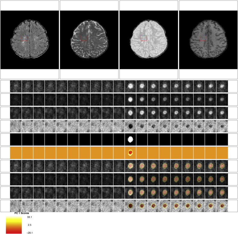
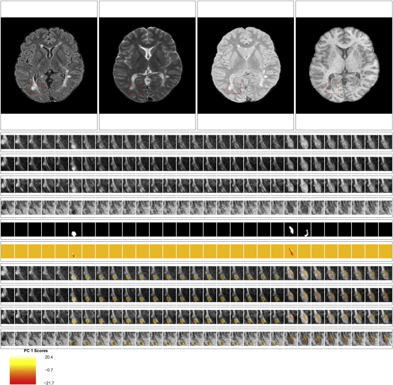
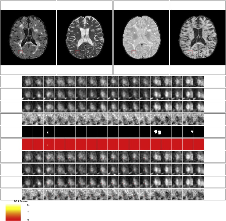
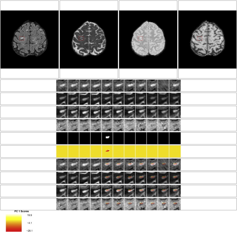
Examples of the set of evaluation images presented to the experts for each lesion are shown in Fig. 9, Fig. 10, Fig. 11, Fig. 12. The first row of the figures shows the full axial slice for the FLAIR, T2, PD, and T1 volumes that contains the largest number of voxels with abnormal signal intensity. The second through fourth rows show the entire collection of longitudinal scans for a box containing the abnormal signal intensity in the FLAIR, T2, PD, and T1 weighted volumes at the baseline time point for this axial slice. The scans are displayed in chronological order, from first time point to last time point, from left to right. The fifth row shows the segmentation of the lesion and edema tissue within this box at each time point. The sixth row shows the score on the first PC for the voxels segmented as lesion tissue, displayed at the time of lesion incidence for each voxel. The seventh through tenth row show the entire collection of longitudinal scans for the FLAIR, T2, PD, and T1 weighted volumes within this box, with the score for the first PC overlaid on the images for each scan after lesion incidence. The last row shows the scale for the score on the first PC. The figures show examples of the four different ratings for the score on the first PC. Both raters rate the scans as either (1) failed miserably, (2) some redeeming features, (3) passed with minor errors, or (4) passed.

Fig. 9.

Passed: rating of 4 for the score on the first PC. This scan received a rating of 4 for the score on the first PC from both raters. Both raters also gave a rating of 4 for the lesion segmentation.

Fig. 10.

Passed with minor errors: rating of 3 for the score on the first PC. This scan received a rating of 3 for the score on the first PC from both raters. Both raters also gave a rating of 3 for the lesion segmentation. Note that at the 23rd time point new lesion voxels are segmented, but the score for the first PC is not produced for this time point, as the voxels did not meet the scanning criteria for being included in the analysis.

Fig. 11.

Some redeeming features: rating of 2 for the score on the first PC. This scan received a rating of 2 for the score on the first PC from both raters. Both raters also gave a rating of 2 for the lesion segmentation. The neuroradiologist commented that this scan received a low rating because it was not clear that the segmented portion for time point 3 was lesion.

Fig. 12.

Failed miserably: rating of 1 for the score on the first PC. This scan received a rating of 1 for the score on the first PC from both raters. Both raters also gave a rating of 1 for the lesion segmentation. Both raters commented that the low rating was because the lesion had existed in all time points and was not a new lesion.

A.8. Principal component analysis and regression

Table 2

Table 2.

Coefficient estimates, standard errors, t-statistics, p-values, and bootstrapped 95% confidence intervals for the multivariate PCA regression model.

	Estimate	Standard error	t-Value	p-Value	95% bootstrapped CI
SPMS	2.15	4.41	0.49	0.63	(− 6.19, 10.93)
Distance to boundary	− 9.39	0.08	− 123.74	0.00	(− 9.56, − 9.25)
Age	− 0.21	0.18	− 1.16	0.25	(− 0.57, 0.13)
(Age − 4)+	-0.10	0.23	-0.42	0.68	(− 0.54, 0.35)
Steroids	4.26	0.79	5.42	0.00	(2.67, 5.85)
Male	1.16	2.55	0.45	0.65	(− 3.94, 6.61)
Treatment	5.39	0.36	15.03	0.00	(4.67, 6.08)
Intercept	8.89	1.92	4.64	0.00	(5.17, 12.85)

shows the coefficient estimates, standard errors, t-statistics, the p-values using the normal approximation, and the 95% bootstrapped confidence intervals for the multivariate PCA regression model. Table 3

Table 3.

Coefficient estimates, standard errors, t-statistics, p-values, and bootstrapped 95% confidence intervals for the univariate PCA regression model.

	Estimate	Standard error	t-Value	p-Value	95% bootstrapped CI
SPMS	0.65	4.11	0.16	0.88	(− 7.71, 9.18)
Distance to boundary	− 9.37	0.08	− 123.18	0.00	(− 9.52, − 9.22)
Age	0.89	0.19	4.58	0.00	(0.51, 1.23)
(Age − 4)+	− 1.55	0.24	− 6.40	0.00	(− 1.95, − 1.14)
Steroids	6.03	0.78	7.77	0.00	(4.55, 7.59)
Male	0.43	2.43	0.18	0.86	(− 4.32, 4.97)
Treatment	4.48	0.38	11.76	0.00	(3.67, 5.25)

shows the same for the individual univariate PCA regression models.

A.9. Function-on-scalar regression

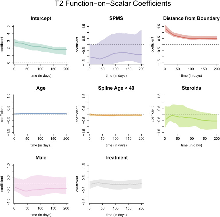
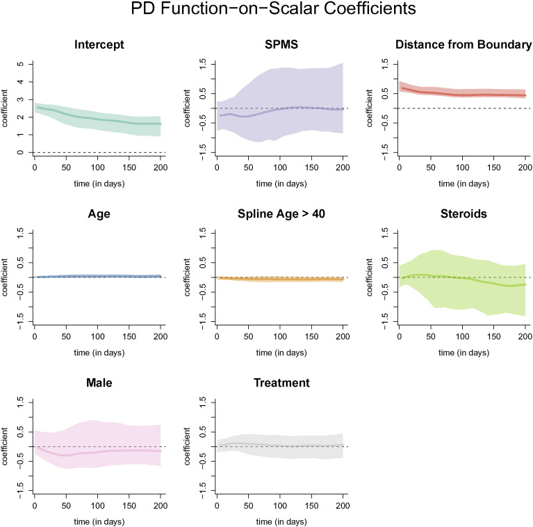
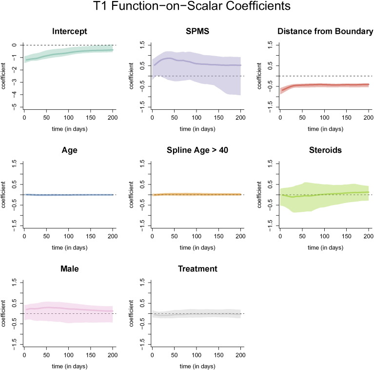
The coefficient functions from the function-on-scalar regression with bootstrapped 95% confidence intervals with the T2, PD, and T1 profile as the outcome are shown below. Similar to using the FLAIR profile as the outcome, only the distance to the boundary and age were found to be different from 0 at any point along the profile (Fig. 13, Fig. 14, Fig. 15).

Fig. 13.

Coefficient functions from the function-on-scalar regression with the T2 profile as an outcome. Each dark line represents the coefficient function, and the shaded area represents a bootstrapped, point-wise 95% confidence interval. Along the y-axis is the value of the coefficient function at each time point. Only distance from the boundary and age were found to be different from 0 at any point along the profile.

Fig. 14.

Coefficient functions from the function-on-scalar regression with the PD profile as an outcome. Each dark line represents the coefficient function, and the shaded area represents a bootstrapped, point-wise 95% confidence interval. Along the x-axis of each plot is the time in days from lesion incidence. Along the y-axis is the value of the coefficient function at each time point. Only distance from the boundary and age were found to be different from 0 at any point along the profile.

Fig. 15.

Coefficient functions from the function-on-scalar regression with the T1 profile as an outcome. Each dark line represents the coefficient function, and the shaded area represents a bootstrapped, point-wise 95% confidence interval. Along the x-axis of each plot is the time in days from lesion incidence. Along the y-axis is the value of the coefficient function at each time point. Only distance from the boundary and age were found to be different from 0 at any point along the profile.

References

- Barkhof F. The clinico-radiological paradox in multiple sclerosis revisited. Curr. Opin. Neurol. 2002;15(3):239–245. doi: 10.1097/00019052-200206000-00003. [DOI] [PubMed] [Google Scholar]
- Barr D.J., Levy R., Scheepers C., Tily H.J. Random effects structure for confirmatory hypothesis testing: keep it maximal. J. Mem. Lang. 2013;68(3):255–278. doi: 10.1016/j.jml.2012.11.001. [DOI] [PMC free article] [PubMed] [Google Scholar]
- Carass A., Wheeler M.B., Cuzzocreo J., Bazin P.-L., Bassett S.S., Prince J.L. Biomedical Imaging: From Nano to Macro, 2007. ISBI 2007. 4th IEEE International Symposium on. IEEE; 2007. A joint registration and segmentation approach to skull stripping; pp. 656–659. [Google Scholar]
- Crainiceanu C., Reiss P., Goldsmith J., Huang L., Huo L., Scheipl F. R Package Version. 2014. Refund: regression with functional data; pp. 1–11. [Google Scholar]
- Efron B., Tibshirani R.J. CRC Press; 1994. An Introduction to the Bootstrap. [Google Scholar]
- Fan J., Zhang J.-T. Two-step estimation of functional linear models with applications to longitudinal data. J. R. Stat. Soc. Ser. B Stat Methodol. 2000;62(2):303–322. [Google Scholar]
- Filippi M., Iannucci G., Cercignani M., Rocca M.A., Pratesi A., Comi G. A quantitative study of water diffusion in multiple sclerosis lesions and normal-appearing white matter using echo-planar imaging. Arch. Neurol. 2000;57(7):1017–1021. doi: 10.1001/archneur.57.7.1017. [DOI] [PubMed] [Google Scholar]
- Filippi M., Cercignani M., Inglese M., Horsfield M., Comi G. Diffusion tensor magnetic resonance imaging in multiple sclerosis. Neurology. 2001;56(3):304–311. doi: 10.1212/wnl.56.3.304. [DOI] [PubMed] [Google Scholar]
- Fonov V., Evans A., McKinstry R., Almli C., Collins D. Unbiased nonlinear average age-appropriate brain templates from birth to adulthood. NeuroImage. 2009;47:S102. [Google Scholar]
- Ghassemi R., Brown R., Banwell B., Narayanan S., Arnold D.L. Quantitative measurement of tissue damage and recovery within new t2w lesions in pediatric-and adult-onset multiple sclerosis. Mult. Sclerosis J. 2014;21(6):718–725. doi: 10.1177/1352458514551594. [DOI] [PubMed] [Google Scholar]
- Lucas B.C., Bogovic J.A., Carass A., Bazin P.-L., Prince J.L., Pham D.L., Landman B.A. The java image science toolkit (JIST) for rapid prototyping and publishing of neuroimaging software. Neuroinformatics. 2010;8(1):5–17. doi: 10.1007/s12021-009-9061-2. [DOI] [PMC free article] [PubMed] [Google Scholar]
- McCulloch C.E., Neuhaus J.M. Wiley Online Library; 2001. Generalized Linear Mixed Models. [Google Scholar]
- McFarland H., Barkhof F., Antel J., Miller D. The role of MRI as a surrogate outcome measure in multiple sclerosis. Mult. Scler. 2002;8(1):40–51. doi: 10.1191/1352458502ms767xx. [DOI] [PubMed] [Google Scholar]
- Meier D.S., Guttmann C.R. Time-series analysis of MRI intensity patterns in multiple sclerosis. NeuroImage. 2003;20(2):1193–1209. doi: 10.1016/S1053-8119(03)00354-9. [DOI] [PubMed] [Google Scholar]
- Meier D.S., Guttmann C.R. MRI time series modeling of ms lesion development. NeuroImage. 2006;32(2):531–537. doi: 10.1016/j.neuroimage.2006.04.181. [DOI] [PubMed] [Google Scholar]
- Meier D.S., Weiner H.L., Guttmann C.R. Time-series modeling of multiple sclerosis disease activity: a promising window on disease progression and repair potential? Neurotherapeutics. 2007;4(3):485–498. doi: 10.1016/j.nurt.2007.05.008. [DOI] [PMC free article] [PubMed] [Google Scholar]
- Polman C.H., Reingold S.C., Banwell B., Clanet M., Cohen J.A., Filippi M., Fujihara K., Havrdova E., Hutchinson M., Kappos L. Diagnostic criteria for multiple sclerosis: 2010 revisions to the McDonald criteria. Ann. Neurol. 2011;69(2):292–302. doi: 10.1002/ana.22366. [DOI] [PMC free article] [PubMed] [Google Scholar]
- R Development Core Team . R Foundation for Statistical Computing; Vienna, Austria: 2008. R: A Language and Environment for Statistical Computing. [Google Scholar]
- Reich D.S., White R., Cortese I.C., Vuolo L., Shea C.D., Collins T.L., Petkau J. Sample-size calculations for short-term proof-of-concept studies of tissue protection and repair in multiple sclerosis lesions via conventional clinical imaging. Mult. Sclerosis J. 2015;21(13):1693–1704. doi: 10.1177/1352458515569098. [DOI] [PMC free article] [PubMed] [Google Scholar]
- Shiee N., Bazin P.-L., Ozturk A., Reich D.S., Calabresi P.A., Pham D.L. A topology-preserving approach to the segmentation of brain images with multiple sclerosis lesions. NeuroImage. 2010;49(2):1524–1535. doi: 10.1016/j.neuroimage.2009.09.005. [DOI] [PMC free article] [PubMed] [Google Scholar]
- Shinohara R.T., Crainiceanu C.M., Caffo B.S., Gaitán M.I., Reich D.S. Population-wide principal component-based quantification of blood–brain-barrier dynamics in multiple sclerosis. NeuroImage. 2011;57(4):1430–1446. doi: 10.1016/j.neuroimage.2011.05.038. [DOI] [PMC free article] [PubMed] [Google Scholar]
- Shinohara R.T., Sweeney E.M., Goldsmith J., Shiee N., Mateen F.J., Calabresi P.A., Jarso S., Pham D.L., Reich D.S., Crainiceanu C.M. Statistical normalization techniques for magnetic resonance imaging. NeuroImage Clin. 2014;6:9–19. doi: 10.1016/j.nicl.2014.08.008. [DOI] [PMC free article] [PubMed] [Google Scholar]
- Sweeney E., Shinohara R., Shea C., Reich D., Crainiceanu C. Automatic lesion incidence estimation and detection in multiple sclerosis using multisequence longitudinal MRI. Am. J. Neuroradiol. 2013;34(1):68–73. doi: 10.3174/ajnr.A3172. [DOI] [PMC free article] [PubMed] [Google Scholar]
- Sweeney E.M., Shinohara R.T., Shiee N., Mateen F.J., Chudgar A.A., Cuzzocreo J.L., Calabresi P.A., Pham D.L., Reich D.S., Crainiceanu C.M. Oasis is automated statistical inference for segmentation, with applications to multiple sclerosis lesion segmentation in MRI. NeuroImage Clin. 2013;2:402–413. doi: 10.1016/j.nicl.2013.03.002. [DOI] [PMC free article] [PubMed] [Google Scholar]
- Van Waesberghe J., Kamphorst W., De Groot C.J., Van Walderveen M.A., Castelijns J.A., Ravid R., Lycklama a Nijeholt G., Van Der Valk P., Polman C.H., Thompson A.J. Axonal loss in multiple sclerosis lesions: magnetic resonance imaging insights into substrates of disability. Ann. Neurol. 1999;46(5):747–754. doi: 10.1002/1531-8249(199911)46:5<747::aid-ana10>3.3.co;2-w. [DOI] [PubMed] [Google Scholar]
- Whitcher B., Schmid V.J., Thornton A. Working with the DICOM and NIfTI data standards in R. J. Stat. Softw. 2011;44(6):1–28. [Google Scholar]