Functional Module Analysis for Gene Coexpression Networks with Network Integration

Abstract

Network has been a general tool for studying the complex interactions between different genes, proteins and other small molecules. Module as a fundamental property of many biological networks has been widely studied and many computational methods have been proposed to identify the modules in an individual network. However, in many cases a single network is insufficient for module analysis due to the noise in the data or the tuning of parameters when building the biological network. The availability of a large amount of biological networks makes network integration study possible. By integrating such networks, more informative modules for some specific disease can be derived from the networks constructed from different tissues, and consistent factors for different diseases can be inferred.

In this paper, we have developed an effective method for module identification from multiple networks under different conditions. The problem is formulated as an optimization model, which combines the module identification in each individual network and alignment of the modules from different networks together. An approximation algorithm based on eigenvector computation is proposed. Our method outperforms the existing methods, especially when the underlying modules in multiple networks are different in simulation studies. We also applied our method to two groups of gene coexpression networks for humans, which include one for three different cancers, and one for three tissues from the morbidly obese patients. We identified 13 modules with 3 complete subgraphs, and 11 modules with 2 complete subgraphs, respectively. The modules were validated through Gene Ontology enrichment and KEGG pathway enrichment analysis. We also showed that the main functions of most modules for the corresponding disease have been addressed by other researchers, which may provide the theoretical basis for further studying the modules experimentally.

I. INTRODUCTION

WITH the fast development of high-throughput technologies, a huge amount of different types of data are available, which include gene expression data, sequence data, genotype data, and some others. This makes it possible for researchers to study the complex relations between different genes/proteins such as coexpression, regulation, and interaction, and so on. A general tool for such studies is network, where the nodes correspond to the genes or proteins, and the edges represent the relations between them. By studying the properties of the networks, we can infer the useful information of the complex biological systems. Many works on this topic have been published in recent years [1], [2], [3], [4], [5], [6], [7], [8], [9], [10], [11], [12], [13], [14].

Module structure is a common property of many different types of networks. Intuitively, a module is a densely connected subnetwork within a broader network. In biological networks, the genes or proteins in the same module are more likely to share some common properties or play similar roles [2], [4], [10]. By dividing the networks into modules, a large system can be reduced, and we can further study the properties of the modules, or we can infer the functions of the unknown genes based on the other genes’ function in the same module. A lot of papers have been published to address the functional module identification for an individual biological network or one general network [15], [16], [17], [18], [19], [20], [21], [22], [23], [24].

Although many computational methods have been proposed to study the modules in an individual biological network, in many cases the modules in a single network may not be stable due to the noise in the data or the tuning of parameters when building the networks. The availability of a large amount of biological networks makes network integration study possible. By integrating networks for different species, we can study the conservation and evolvement relations of them. Integration of networks for the same species under multiple conditions may reveal their pattern differences. For example, by integrating the networks constructed from case and control data, we may find the main disease causal subnetworks. These facts lead to the great need of the development of related computational and statistical methods. A few methods have been proposed to find the densely connected subgraphs from multiple biological networks [25], [26], [27], [28]. These methods mainly used heuristic algorithms to do subgraph searching, where the search space is reduced step by step. They are more likely to find the small subgraphs compared to the general concept of modules. The module identification problem from multislice networks has not been addressed until recently [29]. There, the authors generalized the framework of network quality functions in [30], where the popular quantitative module measure ‘modularity’ is proposed, to study the module structure of multislice networks. Later on, Zhang [31] proposed an optimization algorithm to rapidly detect common module structure in time-varying networks. As the authors noted in the paper, this method does not perform stably for some networks. Almost at the same time, several papers from machine learning field were also published to study clustering for integrated data [32], [33], [34], [35]. Since these methods mainly used spectral clustering or other graph-based methods, they can be applied to do module identification in integrated networks. However, most of these methods were proposed under the assumption that the underlying modules/clusters for all considered networks/data sets are the same. In reality, the module structures for the considered networks may vary greatly. For example, the gene coexpression networks constructed under different disease conditions may consist of different modules although there may exist consistent modules. These motivate us to study novel methods for module identification from multislice networks, where the modules may have different sizes.

In this article, we focus on the module analysis for multislice biological networks, in particular, the gene coexpression networks. By identifying the consistent modules in such networks constructed from patients having different diseases, we can obtain the common factors of them. Identification of consistent modules from the gene coexpression networks for the patients’ different tissues can discover the subtle signals that may not be clear in one specific tissue. In the following, we propose an optimization model to identify the consistent modules across multiple networks. This model combines the module identification in an individual network and module alignment from different networks together. We use spectral clustering to identify the modules from a single network, and the alignment of modules is done by defining the similarity between different modules with cosine. Putting these two terms together, the model is transformed to a trace minimization problem with linear constraints, which can be solved quickly with an approximation method. We demonstrate our method with the simulated networks and compare its performance with some popular existing methods. Our method outperforms other methods, especially when the underlying modules have different sizes. We note that our method can easily handle more than three networks although we only consider the case that there are at most three networks in the paper.

We apply the proposed method to two different types of real data settings. One is for networks constructed from different cancers, the other is for networks from different tissues in morbidly obese patients. Several consistent modules are identified for these two data sets. We validate the results with both Gene Ontology enrichment analysis and KEGG pathway enrichment analysis. More than ten modules enrich the GO terms and KEGG pathways significantly in both data settings. Many of the enriched terms have been addressed by other researchers through experimental study. These results may provide the theoretical basis for further studying the relations between the diseases and the modules experimentally. Further more, although we studied unweighted networks in this paper, our method can be easily extended to weighted networks.

II. METHODOLOGY

Suppose we have K different networks G₁, G₂, ⋯, G_K, which are constructed from gene expression data sets under K different conditions. Each network consists of n nodes. The adjacency matrix for network G_k is A_k, where A_k(i, j) = 1, if there is an edge between node i and node j, otherwise A_k(i, j) = 0. We use D_k to denote the diagonal matrix with the diagonal entries being the degree of the corresponding node. We let M be the putative number of the consistent modules across the K networks, and let S^k be the assignment of the n nodes into M modules for the network G_k, where

$$\begin{array}{l}{S}_{im}^k=\{\begin{array}{l}1,\text{if}i\in G_k\text{belongs to the }m-\text{th module,}\hfill \\ 0,\text{otherwise,}\hfill \end{array}\\ i=1,2,\cdots ,n;m=1,2,\cdots ,M;k=1,2,\cdots ,K.\end{array}$$

A. Module identification in an individual network G_k with spectral clustering

Spectral clustering has been one of the most popular modern clustering techniques in recent years. This method first constructs a similarity graph based on the pairwise distance of all the data points. Then the Laplacian matrix of the graph is computed. The clustering result is obtained by clustering the eigenvectors corresponding to the M smallest eigenvalues of the Laplacian matrix. It can be implemented easily and outperforms the traditional clustering algorithms in many cases. From the graph cut point of view, it is to find a partition of the similarity graph such that the edges between different groups have very low weights and the edges within groups have high weights. The unnormalized spectral clustering corresponds to the RatioCut, where the weight between two groups is the sum of the total number of edges between them normalized by the number of the nodes in each group [36].

Spectral clustering can be directly applied to do module identification for any one network if we take the considered network as the similarity graph. For a given network G_k, we define

$${\mathrm{\Psi }}_k(S^k)={\displaystyle \sum _{m=1}^M\frac{{S_{.,m}^k}^T(D_k-A_k)S_{.,m}^k}{{S_{.,m}^k}^T{S}_{.,m}^k}}$$ (1)

where $S_{.,m}^k$ denotes the m-th column of matrix S^k for the network G_k. Then the corresponding optimization problem is formulated as:

$$\begin{array}{ll}\min \hfill & {\mathrm{\Psi }}_k(S^k)\hfill \\ \mathrm{s}.\mathrm{t}.\hfill & S_{i,m}^k\in \{0,1\},i=1,2,\cdots ,n,m=1,2,\cdots ,M,{\displaystyle \sum _{m=1}^M{S}_{.,m}^k=1,}\hfill \end{array}$$ (2)

where 1 is a vector with all entries being 1.

By letting ${\stackrel{\sim }{S}}_{.,m}^k=\frac{S_{.,m}^k}{{\Vert S_{.,m}^k\Vert }_2}$, the problem is relaxed to:

$$\begin{array}{ll}\min \hfill & {\stackrel{\sim }{\mathrm{\Psi }}}_k({\stackrel{\sim }{S}}^k)=\text{Tr}({\stackrel{\sim }{S}}^{k^T}(D_k-A_k){\stackrel{\sim }{S}}^k)\hfill \\ \mathrm{s}.\mathrm{t}.\hfill & {\stackrel{\sim }{S}}^{k^T}{\stackrel{\sim }{S}}^k=I_M.\hfill \end{array}$$

Let L_k = D_k − A_k, we can use the standard procedure of spectral clustering to get the module label for the network.

B. Integration of multiple networks

To find the consistent modules across multislice networks, we need to align the modules obtained for different networks. If we align the identified modules in each network directly, the computation is complex. Thus we propose to do module identification for each network and alignment of the modules for multiple networks together. To identify the modules in each network, we use spectral clustering. For the alignment of modules in different networks, we expect the same node is clustered to the same module. Then we define the similarity between modules in different networks using cosine. The similarity between the m–th module in network G_k and G_l is defined as $\frac{S_{.,m}^k\cdot S_{.m}^l}{{\Vert S_{.,m}^k\Vert }_2{\Vert S_{.,m}^l\Vert }_2}$. We aim to maximize the similarities of the corresponding modules in all networks, and our objective becomes:

$$\mathrm{\Psi }(S^1,\cdots ,S^K)={\displaystyle \sum _{k=1}^K{\mathrm{\Psi }}_k(S^k)-\beta {\displaystyle \sum _{k,l=1}^K{\displaystyle \sum _{m=1}^M\frac{{S_{,m}^k}^T{S}_{,m}^l}{{\Vert S_{,m}^k\Vert }_2{\Vert S_{,m}^l\Vert }_2}}}},$$

where β is the parameter to control the contributions from the intra- and inter- network connections. The optimization problem is formulated as:

$$\begin{array}{l}C=\left(\begin{array}{llll}{L}_1\hfill & 0\hfill & \cdots \hfill & 0\hfill \\ 0\hfill & L_2\hfill & \cdots \hfill & 0\hfill \\ ⋮\hfill & ⋮\hfill & \ddots \hfill & 0\hfill \\ 0\hfill & 0\hfill & \cdots \hfill & L_K\hfill \end{array}\right)-\beta \left(\begin{array}{llll}0\hfill & I_n\hfill & \cdots \hfill & I_n\hfill \\ I_n\hfill & 0\hfill & \cdots \hfill & I_n\hfill \\ ⋮\hfill & ⋮\hfill & \ddots \hfill & I_n\hfill \\ I_n\hfill & I_n\hfill & \cdots \hfill & 0\hfill \end{array}\right),\hfill \\ \stackrel{\sim }{S}=\left(\begin{array}{c}{\stackrel{\sim }{S}}^1\\ {\stackrel{\sim }{S}}^2\\ ⋮\\ {\stackrel{\sim }{S}}^K\end{array}\right),\hfill \end{array}$$ (3)

We define

$$C=\left(\begin{array}{llll}{L}_1\hfill & 0\hfill & \cdots \hfill & 0\hfill \\ 0\hfill & L_2\hfill & \cdots \hfill & 0\hfill \\ ⋮\hfill & ⋮\hfill & \ddots \hfill & 0\hfill \\ 0\hfill & 0\hfill & \cdots \hfill & L_K\hfill \end{array}\right)-\beta \left(\begin{array}{llll}0\hfill & I_n\hfill & \cdots \hfill & I_n\hfill \\ I_n\hfill & 0\hfill & \cdots \hfill & I_n\hfill \\ ⋮\hfill & ⋮\hfill & \ddots \hfill & I_n\hfill \\ I_n\hfill & I_n\hfill & \cdots \hfill & 0\hfill \end{array}\right),\stackrel{\sim }{S}=\left(\begin{array}{c}{\stackrel{\sim }{S}}^1\\ {\stackrel{\sim }{S}}^2\\ ⋮\\ {\stackrel{\sim }{S}}^K\end{array}\right),$$

and L_k = D_k − A_k, 0 is an n × n matrix with all entries being zero.

With the same technique as spectral clustering, the above optimization problem is relaxed to:

$$\begin{array}{ll}\min \hfill & \stackrel{\sim }{\mathrm{\Psi }}(\stackrel{\sim }{S})=\text{Tr}({\stackrel{\sim }{S}}^{T}C\stackrel{\sim }{S})\hfill \\ \mathrm{s}.\mathrm{t}.\hfill & {\stackrel{\sim }{S}}^T\stackrel{\sim }{S}=K{I}_M.\hfill \end{array}$$

In this formulation, the constant coefficient K can be put into C, such that each column of $\stackrel{\sim }{S}$ has the norm 1. We take $\stackrel{\sim }{S}$ as a data set composed of Kn nodes and do k–means clustering, we can get the assignment label for each node. Then we put the nodes back to each network and see the consistent elements in each module. The algorithm is summarized in the following.

Algorithm

Input: Adjacency matrix A_k, k = 1, 2 ⋯, K, and M, which is the putative number of consistent modules.

1. Compute the matrices L_k = D_k − A_k, k = 1, 2, ⋯, K;

2. Construct the matrix C;

3. Compute the M eigenvectors v₁, v₂, ⋯, v_M corresponding to the M smallest eigenvalues of matrix C;

4. Construct a new matrix T ∈ R^Kn×M, with columns v₁, v₂, ⋯, v_M;

5. Cluster the points constructed from each row of matrix T with k-means clustering into clusters C₁, C₂, ⋯, C_M;

6. For each cluster, divide the points into K sets according to their original network label, find the consistent points of these sets.

Output: Index of nodes in each consistent module.

The algorithm is similar to spectral clustering procedure. The two main steps are computation of eigenvectors and k-means clustering. A direct eigen-decomposition takes O((Kn)³) time, and has a space complexity O(Kn²), where n is the size of the similarity matrix. By using sampling techniques [37], the time complexity can be reduced to O(KnpM) where M is the number of eigenvectors to be computed, p is the number of sampling points where can be chosen to be significantly less than Kn. The space complexity is also reduced to O(KMn). When we perform k-means clustering, we only need M eigenvectors. The running time of the algorithm is about O(KnM²I), where I is the number of iterations required for convergence [37].

With this algorithm, we can both identify the modules in each network (the sizes of modules can be different) and the consistent modules across multislice networks. The cosine similarity between the corresponding modules in different networks helps align the modules. Here, M is prespecified as the putative number of consistent modules across all the considered networks. In practice, the nodes of some module may not be connected densely. Thus we need to check the structure of these clustered nodes to make sure the consistent modules are all densely connected subnetworks in each network.

III. RESULTS

In this section, we first use simulated networks to demonstrate our method. We then apply it to two real data sets to identify the meaningful modules.

A. Simulation Study

1) Demonstration of our method with synthetic data

To objectively evaluate the performance of our proposed method, we tested it on a synthetic gene expression data set. The data sets, available at http://tsenglab.biostat.pitt.edu/publication.htm, were used to evaluate many clustering algorithms in a previous study [38]. Each data set contains simulated expression data under 50 conditions. Each gene was pre-assigned to one of fifteen clusters, and the expression profiles for the genes in the same cluster were from a common log normal distribution. Gaussian noise was then added to the data set to simulate experimental noise. The different standard deviations of the noise may represent the different data collection conditions such as different labs, or different tissues. We choose five groups ‘data_i_Noise0._SD…txt’, where i is 0,1,2,3,4, and SD is 0.2, 0.4, and 0.8 in each group. We then find the largest cluster for the data with SD=0.2, and choose the other two clusters with the mean absolute value of the correlation coefficient being closest to the selected one. By choosing the clusters in this way, we try to make sure that the module structure of the network is clear. Finally, in each data set, there are three clusters, which correspond to the three modules in our constructed network.

To construct the gene coexpression network, we use hard thresholding, that is, if the absolute value of the correlation coefficient is greater than the threshold, we assign an edge between the corresponding nodes. Here, the networks are unweighted, that is when there is an edge, the corresponding value in the adjacency matrix is set to 1. To choose the threshold, we first compute the mean absolute value of the correlation coefficients for the three networks, and record the maximum value among them. We then divide the value from 0.5 to 1 into 10 intervals with equal stepsize. The threshold is chosen to be the endpoint of the 10 intervals that is closest to the recorded maximum value. With this strategy, the module structure is clear and the number of isolated nodes is not large.

We conducted numerical experiments for these networks with our proposed method. In this example, we directly set β = 1. To compare the results with that of module identification in each individual network, we applied the method proposed in [23] because this method has shown to outperform most methods and it pays more attention to the large modules instead of isolated nodes. In all these experiments, K is chosen to be 3. The results are shown in Table I. In the table, ‘Cluster’ is the three chosen clusters among the fifteen clusters in each data set, ‘α’ is the threshold for building the networks. ‘No_isolated’ is the number of isolated nodes in each network, ‘Accu_sep’ shows the identification accuracy when we did module identification in each network separately, and ‘Accu_int’ shows the identification accuracy with our proposed method. Module identification with network integration achieves the highest identification accuracy in all the tests. Since the simulated data sets have very clear module structure, in some cases, module identification in an individual network also achieves good performance. However, when there are several isolated nodes, with network integration, we can combine all the information together and get better performance. Take as an example, we plotted the identification results for ‘data_0_Noise0._SD…txt’ in Fig. 1, where the three different colors, in the three networks represent our identified consistent modules. Fig. 1(a), 1(b), 1(c) show the network structure under the three different conditions. If we do module identification in the networks individually, the isolated genes will not be assigned correctly. By network integration, we combined the information from the different networks, and all the modules are identified with a high accuracy. The network in Fig. 1(d) includes all the edges in the three networks. This example shows that module identification by network integration can give better results compared to that from an individual network.

TABLE I.

MODULE IDENTIFICATION RESULTS FOR THE SIMULATED DATA.

data	SD	Cluster	α	Noisolated	Accusep	Accuint
data_0 _Noise0.	0.2	0,6,8	0.85	19	0.88	0.97
	0.4		0.70	6	0.95
	0.8		0.50	7	0.91
data_1 _Noise0.	0.2	1,4,6	0.85	0	0.99	1.00
	0.4		0.75	8	0.91
	0.8		0.55	16	0.96
data_2 _Noise0.	0.2	8,12,13	0.85	0	0.99	1.00
	0.4		0.70	4	0.91
	0.8		0.50	15	0.78
data_3 _Noise0.	0.2	4,11,12	0.90	0	1.00	1.00
	0.4		0.80	5	0.91
	0.8		0.60	8	0.93
data_4 _Noise0.	0.2	1,2,10	0.80	1	0.97	1.00
	0.4		0.65	8	0.79
	0.8		0.50	29	0.55

’SD’ is the standard deviation of the noise, ’α’ is the cutoff for building the gene coexpression networks, ’No_isolated’ is the number of isolated nodes in each network, ’Accu_sep’ is the identification accuracy for each individual network, ’Accu_int’ is the identification accuracy using the integration method.

Fig. 1.

Module identification from three synthetic gene coexpression networks. The different colors show the three modules. (a, b, c): The networks under three different conditions; (d): The network with edges including all the edges in the three networks.

2) Comparison with existing methods

In this subsection, we will compare our method with some existing methods through simulation studies. The comparison methods include: (1) Affinity Aggregation for Spectral Clustering (AASC) [32]; (2) Co-Regularized multi-view Spectral Clustering (CRSC) [33]; (3) Nonnegative Matrix Factorization based Clustering method (NMFC) [31]; and (4) Optimized data fusion for K-means Laplacian Clustering (OKLC) [34].

The networks are randomly generated following the stochastic block model [39]. We first assign a number of nodes to three modules such that each module has the given number of nodes. Then the connections within and between different modules are generated according to a given probability matrix, in which the diagonal entries specify the connection probabilities within the modules and the other entries specify the connection probabilities between the corresponding modules. We consider the following four connection probabilities with the probabilities between different modules increasing:

$$\begin{array}{l}{P}_1=\frac{1}{n}\left(\begin{array}{lll}16\hfill & 0\hfill & 0\hfill \\ 0\hfill & 18\hfill & 0\hfill \\ 0\hfill & 0\hfill & 17\hfill \end{array}\right),P_2=\frac{1}{n}\left(\begin{array}{lll}16\hfill & 0.4\hfill & 0.6\hfill \\ 0.4\hfill & 18\hfill & 0.55\hfill \\ 0.6\hfill & 0.55\hfill & 17\hfill \end{array}\right),\\ P_3=\frac{1}{n}\left(\begin{array}{lll}16\hfill & 0.8\hfill & 1.2\hfill \\ 0.8\hfill & 18\hfill & 1.1\hfill \\ 1.2\hfill & 1.1\hfill & 17\hfill \end{array}\right),P_4=\frac{1}{n}\left(\begin{array}{lll}16\hfill & 1.2\hfill & 1.8\hfill \\ 1.2\hfill & 18\hfill & 1.65\hfill \\ 1.8\hfill & 1.65\hfill & 17\hfill \end{array}\right).\end{array}$$

For each generation probability matrix, we consider the consistent modules for randomly generated network pairs. For the size of the modules, we consider two different settings. One is that the module size is the same for the randomly generated network pairs. We take the module size to be (50,50,50). The other is that the module size is different for the randomly generated network pairs. The module size is set to be (50, 50, 50) and (30, 90, 30). We generated 50 network pairs for each setting and computed the identification accuracy of the consistent modules. This identification accuracy is defined as: $\frac{TP+TN}{TP+TN+FP+FN}$, where ‘TP’, ‘TN’, ‘FP’, and ‘FN’ represent the number of the true positive, true negative, false positive, and false negative.

The results are shown in Table II and Table III. We listed the mean identification accuracy for 50 randomly generated network pairs and the standard deviation in the bracket for each setting. When the module sizes are the same for the network pairs, all the methods have comparable performance, with AASC and our method performing the best. However, as shown in Table III, when the module sizes are different for the network pairs, our method outperforms all the other methods. The main reason is that most of the other methods formulated the optimization problem under the assumption that the module sizes are the same across different networks. Then they focus on finding the common features of the modules to do clustering. For example, in AASC, the M vectors that minimize the ratio cut of the weighted combination of all the networks are computed. By clustering these M vectors, the common modules for all the considered networks can be obtained. Similar techniques are applied in NMFC and OKLC. With such formulations, the module differences between each network pair cannot be identified. In NMFC, although a different method for determining the common modules is given, it is not stable as mentioned by the authors. Compared to these three methods, CRSC considers both the intra-network module structures and module similarities between different netwoks. The modules in each network are identified by normalized spectral clustering, and the consistent module structure is defined by a similarity function, which is similar to our method. However, since the formulated optimization problem is solved by an iterative method, which alternatively computes the eigenvectors of a regularized Laplacian matrix, it is more likely to get the local maximum solution, and thus it is not stable. We note that in CRSC and our method, we vary the regularization parameter between 0.2 to 3, and report the best identification accuracy. Also we need to mention that CRSC is slower than our method due to the iteration process for solving the optimization problem.

TABLE II.

COMPARISON OF THE IDENTIFICATION ACCURACY FOR THE NETWORKS WITH THE SAME MODULE SIZES ACROSS DIFFERENT NETWORKS.

Setting	P1	P2	P3	P4
AASC	1.00(0.00)	1.00(0.00)	1.00(0.00)	1.00(0.01)
CRSC	1.00(0.01)	0.99(0.01)	0.99(0.01)	0.96(0.08)
NMFC	0.96(0.08)	0.97(0.07)	0.97(0.06)	0.98(0.05)
OKLC	0.99(0.01)	0.99(0.01)	0.99(0.01)	0.98(0.03)
Our method	1.00(0.00)	1.00(0.00)	1.00(0.00)	1.00(0.01)

TABLE III.

COMPARISON OF THE IDENTIFICATION ACCURACY FOR THE NETWORKS WITH DIFFERENT MODULE SIZES ACROSS DIFFERENT NETWORKS.

Setting	P1	P2	P3	P4
AASC	0.72(0.01)	0.71(0.01)	0.72(0.01)	0.72(0.01)
CRSC	0.73(0.00)	0.73(0.01)	0.72(0.01)	0.72(0.01)
NMFC	0.69(0.08)	0.68(0.03)	0.66(0.04)	0.65(0.04)
OKLC	0.67(0.10)	0.68(0.08)	0.66(0.09)	0.65(0.10)
Our method	1.00(0.00)	0.98(0.01)	0.93(0.08)	0.80(0.13)

3) Selection of the parameter β

In our proposed model, different values of the parameter β may affect the module identification results. We use the same simulation settings as that in the previous subsection, and choose different values for β to see the identification accuracy. β is chosen to be values from 0.2 to 3 with a stepsize 0.2. For each value of β, we simulated 50 network pairs with the module size being (50, 50, 50) and (30, 90, 30), and computed the average identification accuracy. The results are shown in Fig.2. For P₁, the best identification accuracy is obtained when β = 0.2. Because there are no connections between different modules, a small value of β gave the best result. The increase of the connection probability between different modules in each network requires a larger β to make the identification better and stable. For both P₂ and P₃, the best results are obtained when β = 1. And when β becomes larger, the identification accuracy decreases. For P₄, the best results are obtained when β = 2, and the identification accuracy for β = 1 ranks the third (0.76) for all the considered β. When β is larger than 2.4, the identification accuracy becomes smaller. If the generation probabilities between different modules is not very large, it can be seen that a β value of 1 should be a reasonable choice.

Fig. 2.

The average identification accuracy for different values of β.

B. Consistent Module Analysis for Gene Coexpression Networks

1) Gene coexpression networks for different cancers

Network construction

We downloaded the gene expression data from The Cancer Genome Atlas (TCGA) for three cancers: ovarian cancer (OV), glioblastoma multiforme (GBM), and lung squamous cell carcinoma (LUSC) from TCGA website. These data are all generated with Affymetrix HT_HG-U133A by Broad Institute. There are 558 OV samples, 594 GBM samples, and 134 LUSC samples. For each cancer, we computed the variance of all the genes across the samples, and selected the 1500 genes with the largest variance. Then we took the union of the genes for further study. The total number of genes considered is 2756.

To construct the gene coexpression networks, we first calculated the Pearson correlation coefficient between any two genes. Then we constructed the adjacency matrix by hard thresholding. If the absolute value of the Pearson correlation coefficient between two genes is greater than some given value, we assign an edge between them; otherwise, there is no edge. We tried different thresholds and compute the linear regression coefficient between the frequency of degree d (log 10(f(d))) and the log 10 transformed degree d (log 10(d)) to see whether these networks have approximately scale free property as described in [40]. We took the threshold for OV, GBM, and LUSC to be 0.65, 0.52, and 0.60, respectively, to do the hard thresholding, and the average degree for each network is about 18. We then removed the common genes that have no connections to any other genes. Finally, we have three networks with a total number of 2297 genes.

Consistent module analysis

We applied our proposed method to identify all the consistent modules. We directly set β = 1, which has shown to be a reasonable value if the connections between different modules are sparse. For a given M, after the basic steps of our algorithm, we set the size of each module to be greater than 5 and the mean of the average degree for each module in these three cancers to be at least 2 to make sure the identified modules are meaningful. Because with our proposed method, each node must belong to one module, there are some isolated nodes in the modules. We removed the common isolated nodes before we determined the modules, and the size of the modules may be smaller than 5.

In our experiments, after we got the eigenvalues of the matrix C, we computed $\frac{{\lambda }_{i+1}-{\lambda }_i}{{\lambda }_i-{\lambda }_{i-1}}$ with the eigenvalues λ_i satisfying λ₁ ≥ λ₂⋯ ≥λ_N. We then took the first big jump of all the ratio to be the reference for choosing M. We plot the largest 800 eigenvalues for the constructed matrix C as shown in Fig.3. The first big jump appears in the 223-th eigenvalue. To make the results more robust, we tried different M between 150 and 250 and determined the consistent modules that appeared for all these M as the final modules. We finally identified 13 modules. The basic information of these modules is shown in Table IV, where NA means this module belongs to one gene family. We did enrichment analysis for Gene Ontology (GO, biological process) and KEGG pathways for these modules with DAVID [41], [42]. Among these modules, there are three complete graphs in all three cancers including Module 2, Module 9, and Module 11. Module 2 and Module 11 correspond to the gene family GAGE, and CD24(CD24L4), respectively. For the rest modules, 9 among 10 modules enriched GO terms, and 5 of them enriched KEGG pathways. We list all the enrichment results in our supplementary materials¹. The structure of Module 1, 4, 5, 6, 10, and 12 is shown in Fig. 6, where the size of the nodes represents its total degree in the three networks, and the width of the edges represents the total connections between the corresponding nodes in the three networks. We put the same information of Module 3, Module 8, and Module 13 in the supplementary materials because these modules are large.

Fig. 3.

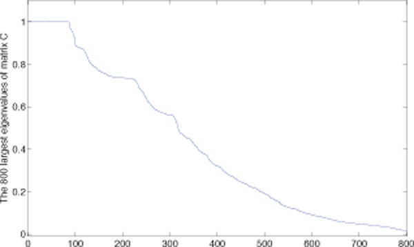
The 800 largest eigenvalues of the matrix C constructed from the cancer data set.

TABLE IV.

MODULE INFORMATION FOR MULTIPLE CANCERS

Module	Size	Density	NGO	NKEGG
Module 1	12	0.6566	15	1
Module 2	6	1.0000	NA	NA
Module 3	41	0.6858	104	4
Module 4	14	0.4359	7	0
Module 5	11	0.8788	2	0
Module 6	7	0.6190	15	2
Module 7	8	0.6310	0	0
Module 8	217	0.2033	262	20
Module 9	7	1.0000	0	0
Module 10	11	0.7697	2	0
Module 11	6	1.0000	NA	NA
Module 12	6	0.6858	9	0
Module 13	77	0.7412	16	3

Fig. 6.

The identified modules 1, 4, 5, 6, 10, 12 for the networks constructed from humans having different cancers. The size of the nodes represents the degree of the node. The width of each edge represents its total number among the three cancers.

Among the three complete graph modules, Module 2 and Module 11 correspond to the gene family GAGE, and CD24(CD24L4), respectively. Module 2 is composed of the probes: 206640_x_at, 207086_x_at, 207663_x_at, 207739_s_at, 208155_x_at, 208235_x_at, which correspond to the genes GAGE3, GAGE4, GAGE5, GAGE6, GAGE7, and GAGE8. These genes all belong to the GAGE family. They are completely silent in normal adult tissues, except testis., but expressed in a variety of tumor tissues [43], [44], such as hepatocellular carcinoma [45], stomach cancer [46], ovarian carcinoma [47], and uterine cervical carcinoma [48]. Fig.4 shows the heatmap of this module for the first 100 samples. In both GBM and LUSC, the gene expressions show similar patterns to that of OV, and several samples have higher expressions. This shows that these genes are also expressed in the GBM and LUSC cancer.

Fig. 4.

Heatmap for Module 2. (a) GBM, (b) OV, (c) LUSC.

Module 11 includes the probes: 208650_s_at, 208651_x_at, 209771_x_at, 209772_s_at, 216379_x_at, and 266_s_at. The genes corresponding to them belong to Cd24 and CD24L4 family. These genes appear to be highly expressed in a large variety of human cancers, such as ovarian cancer [49], nonsmall cell lung cancer [50], colorectal cancer [51], and they have a high correlation with invasiveness [49], [52]. We plotted the heatmap of the genes in this module for the fist 100 samples in Fig.5. The expressions in GBM and LUSC are more similar, and are more highly expressed than that in OV. This may indicate that this module is highly expressed in more human cancers.

Fig. 5.

Heatmap for Module 11. (a) GBM, (b) OV, (c) LUSC.

Another complete graph module is Module 9, which consists of the control probes: AFFX-BioB-3_at, AFFX-BioB-_at, FFX-BioB-M_at, AFFX-BioC-3_at, AFFX-BioC-5_at,AFFX-BioDn-5_at, and AFFX-r2-Ec-bioB-M_at.

The enrichment results with p_value less than 10⁻¹⁰ for GO categories are shown in Table V, where Module 1, 3, 8, and 13 significantly enrich the GO terms. Module 1 consists of a total of 12 genes, which belong to the histone cluster 1 or histone cluster 2. Ten of the twelve genes enrich twelve GO terms, which cover all the genes that belong to these GO terms in our considered gene list. These 10 GO terms are related to chromatin assembly or disassembly, nucleosome assembly, DNA packaging, macromolecular complex assembly and subunit organization, and protein-DNA complex assembly etc, with p_value less than 10⁻¹². Such post-translational histone modifications are known to be altered in cancer cells [53]. Eight of 12 genes enrich the pathway: hsa05322: Systemic lupus erythematosus. Several studies have shown that this pathway is associated with some cancers such as liver cancers, lung cancers, and kidney cancers [54], [55]. Thus it may be worth studying their relations with our considered cancers.

TABLE V.

GENE ONTOLOGY ENRICHMENT OF THE MODULES FOR THE THREE CANCERS

Module	Enriched GO terms	%	pvalue
Module 1	GO:0006334 nucleosome assembly	100	8.83E-21
	GO:0031497 chromatin assembly	100	1.23E-20
	GO:0065004 protein-DNA complex assembly	100	1.88E-20
	GO:0034728 nucleosome organization	100	2.31E-20
	GO:0006323 DNA packaging	100	1.98E-19
	GO:0006333 chromatin assembly or disassembly	100	4.25E-19
	GO:0034622 cellular macromolecular complex assembly	100	1.96E-15
	GO:0034621 cellular macromolecular complex subunit organization	100	5.62E-15
	GO:0006325 chromatin organization	100	9.46E-15
	GO:0051276 chromosome organization	100	9.11E-14
	GO:0065003 macromolecular complex assembly	100	1.59E-12
	GO:0043933 macromolecular complex subunit organization	100	2.88E-12
Module 3	GO:0000278 mitotic cell cycle	57.14	1.31E-22
	GO:0022403 cell cycle phase	57.14	1.12E-21
	GO:0007049 cell cycle	65.71	4.43E-21
	GO:0022402 cell cycle process	60.00	1.01E-20
	GO:0000279 M phase	51.43	4.62E-20
	GO:0000280 nuclear division	45.71	2.14E-19
	GO:0007067 mitosis	45.71	2.14E-19
	GO:0000087 M phase of mitotic cell cycle	45.71	2.82E-19
	GO:0048285 organelle fission	45.71	3.94E-19
	GO:0051301 cell division	40.00	2.81E-14
	GO:0051726 regulation of cell cycle	40.00	1.24E-13
	GO:0007346 regulation of mitotic cell cycle	28.57	3.67E-11
Module 8	GO:0006955 immune response	46.20	3.70E-62
	GO:0006952 defense response	37.43	5.36E-46
	GO:0006954 inflammatory response	23.98	1.89E-31
	GO:0009611 response to wounding	26.90	1.94E-28
	GO:0009615 response to virus	10.53	2.00E-15
	GO:0006959 humoral immune response	9.36	4.56E-15
	GO:0006935 chemotaxis	11.70	7.23E-15
	GO:0042330 taxis	11.70	7.23E-15
	GO:0002504 antigen processing and presentation of peptide or polysaccharide antigen via MHC class II	7.02	2.49E-14
	GO:0002252 immune effector process	10.53	6.84E-14
	GO:0019882 antigen processing and presentation	8.77	2.16E-13
	GO:0002684 positive regulation of immune system process	12.28	1.04E-12
	GO:0045087 innate immune response	9.94	1.60E-12
	GO:0007626 locomotory behavior	12.87	1.61E-12
	GO:0050778 positive regulation of immune response	9.94	3.48E-12
	GO:0002449 lymphocyte mediated immunity	7.60	9.84E-12
	GO:0019724 B cell mediated immunity	7.02	1.55E-11
	GO:0002250 adaptive immune response	7.60	3.19E-11
	GO:0002460 adaptive immune response based on somatic recombination of immune receptors built from immunoglobulin superfamily domains	7.60	3.19E-11
	GO:0002526 acute inflammatory response	8.19	3.85E-11
Module 13	GO:0006955 immune response	40	1.19E-14

Cancer is a disease of inappropriate cell proliferation, and cell cycle machinery controls cell proliferation. The regulation of cell cycle is central to the aberrant cell proliferation for all types of cancers because it lies downstream at the convergence point of complex oncogenic signalling networks. Moreover, because many components in cell cycle are evolutionarily conserved, clinical applications are likely to be suited to diverse tumor types. Many of the current most effective neoadjuvant and adjuvant therapeutic interventions in the clinic are cell cycle directed agents [56]. Module 3 mainly enriches terms related to cell cycle. It enriches 12 GO terms with p_value less than 10⁻¹⁰, and all these 12 terms are related to cell cycle. The most enriched pathway is also cell cycle, with 10 of the 41 genes are involved in it. It may be used as the target gene groups for clinical design in future. More descriptions on the relations between cell cycle and cancer are referred to [57], [56], [58].

When people have cancer, many responses from their body appear to prevent the deterioration. For example, the immune response is generated that results in the proliferation of antigen-specific lymphocytes, which can up-regulate antibodies such that they may better control carcinogenesis, and nowadays immunotherapy has been a new approach to the treatment of cancer [59]. Module 8 and Module 13 are mainly related to different types of responses, such as immune response, defense response, inflammatory response, etc. Some of these responses have been studied, for example, the immune response [59], the defense response [60], and the inflammatory response [61], [62]. The study in stomach cancer shows that besides the marker carbohydrate antigen 19-9(CA19-9), potential markers exist in defense response mechanism [61]. The inflammation as a key event in cancer development is the seventh hallmark of cancer [62]. Inflammatory cells may facilitate angiogenesis and promote the growth, invasion, and metastasis of tumor cells, which link to the genetic instability in cancer cells, which shows that the anti-inflammatory agents should have a potential in both prevention and treatment of cancer. Further study of this module is of great importance for understanding, preventing, and treating cancers.

Comparison with the known cancer-associated genes

We checked the associated genes with these three cancers in KEGG, and found that there is only one common gene tp53, which is translated to the protein p53. This protein regulates the cell cycle in humans, and functions as a tumor suppressor that is involved in preventing cancer. Although this gene is not in our final networks with our construction strategy, we still found its related pathway: hsa04115: p53 signaling pathway, with p_value = 3.57 × 10⁻⁵. Five genes: CDK1, CCNB2, rrm2, CCNB1, and CCNE2 in Module 3 are included in this pathway. In [63], the authors have shown significant change in the DNA copy numbers for gene CCNE1 and CDK4 in GBM. These two genes also belong to this pathway, which validates further that Module 3 should be an important pathway related to cancers. We then took all these cancer-associated genes to see their GO terms enrichment and KEGG pathway enrichment. These genes enrich 166 GO terms, with 65 of them are consistent with those enriched by our identified modules. Among these 65 terms, 2, 25, 6, and 32 terms are from Module 1, Module 3, Module 6, and Module 8, respectively. The most significantly enriched 5 terms of the cancer-associated genes are related to cell cycle. These cancer-associated genes enrich a total of 18 KEGG pathways, with 5 of them may be related to all cancers. Two of them are the same as that enriched by Module 3, which are hsa04115: p53 signaling pathway, and hsa04110: Cell cycle. These suggest that Module 3 plays an important role in all cancers. The extension with more genes in our considered gene list for this module may provide more useful information for cancers. Another notable module is Module 6, which is composed of 7 genes. Although the p_value corresponding to the enriched terms is not very significant, 6 of 15 enriched GO terms are the same as those enriched by the cancer-associated genes. These terms are related to the regulation of kinase activity, transferase activity, and phosphate related processes. Such information suggests that these biological processes may have close relations to cancers.

Comparison with other methods

In the simulation study section, AASC performs the best among the methods that assume the underlying module structures are the same, and CRSC is most similar to our proposed method. Thus we mainly conducted numerical experiments for this data set with these two methods. For CRSC, in each iteration step, we need to compute the eigenvectors of three regularized Laplacian matrices, thus the computation is slow. We did k-means clustering for the obtained eigenvectors after 300 iterations, and used the same method as that in our proposed method to determine the modules. We finally got one module of size 214. This module enriched 108 GO terms and 11 KEGG pathways. There are 27 common genes in this module and Module 8 of our proposed method. The enrichment results are shown in the supplementary materials². For AASC, we also used the same method as that in our method to determine the modules. We obtained 14 modules finally. The module information is shown in Table VI. The enrichment results are shown in the supplementary materials. Table VII shows the modules that were identified with both AASC and our method. ‘N_intersect’ is the number of common genes in the corresponding modules. ‘Similarity’ is defined as the number of common genes in both modules divided by the product of the square root of the number of genes in both modules. Except Module 2, 13 identified by AASC, all the other modules are also identified by our method, with some of them are combined into one module with our method. For example, Module 1 and Module 6 identified by AASC are all included in Module 8 identified by our method. For the genes in Module 2 and 13 identified by AASC, they are distributed in 4 modules when using our method, with some genes in these two modules having the same module label. We checked the subnetwork connections for all the genes in the 4 modules. There are totally 293 genes, of which only 24 genes connected together in all the three networks. And only 14 genes coincide with the genes in Module 2 and Module 13 identified by AASC. Because our method also considers the module structure in each network these 14 genes are assigned to different modules in different networks. Thus our method cannot find this module. By adding all the networks together, AASC identifies the modules directly without considering the information in each network. For Module 4 identified by our method, AASC cannot find it.

TABLE VI.

MODULE INFORMATION FOR MULTIPLE CANCERS WITH AASC

Module	Size	Density	NGO	NKEGG
Module 1	26	0.6708	5	2
Module 2	6	0.8000	8	2
Module 3	68	0.7869	1	0
Module 4	11	0.8788	2	0
Module 5	41	0.6858	104	4
Module 6	7	1.0000	5	0
Module 7	6	0.7111	16	1
Module 8	7	1.0000	0	0
Module 9	9	1.0000	2	0
Module 10	6	1.0000	NA	NA
Module 11	6	1.0000	NA	NA
Module 12	12	0.6566	15	1
Module 13	25	0.5122	11	7
Module 14	332	0.1316	304	23

TABLE VII.

COMMON MODULES OBTAINED WITH OUR METHOD AND AASC

Our method	AASC	Nintersect	Similarity
Module 1	Module 12	12	1.0000
Module 2	Module 10	6	1.0000
Module 3	Module 5	41	1.0000
Module 5	Module 4	11	1.0000
Module 8	Module 14	151	0.5625
Module 9	Module 8	7	1.0000
Module 10	Module 9	9	0.9045
Module 11	Module 11	6	1.0000
Module 12	Module 7	4	0.6667
Module 8	Module 1	26	0.3461
Module 8	Module 6	6	0.1663
Module 13	Module 3	61	0.8430

2) Gene coexpression networks for different tissues of morbidly obese patients

Network construction

This data set collects the gene expression profile of liver, omental and subcutaneous adipose tissues of a large sample of morbidly obese individuals (GEO Accession number: GSE24294). For simplicity, we focused on the 459 subjects with data available for all three tissue types. The original data were measured on 40,638 probes. We identified the genes covered by more than one probe and used the mean expression value as the expression level of that gene. We then excluded the genes with > 10% missing observations and used the mean of the available data to impute the missing values.

After the preprocessing, we got 17,282 common genes of these three tissues. We then selected the first 1,800 most differentially expressed genes of each tissue. We used the union of these genes to construct the gene coexpression network. The total number of genes is 2637.

We used the same method as the previous experiment to construct the gene coexpression network. Here, we took the threshold for obtaining the adjacency matrix to be 0.5. With our choice, all these three networks have the approximately scale-free property, with the $\widehat{R}$ greater than 0.9. The average degree of gene coexpression networks for liver, omental and subcutaneous adipose tissues is 13.2, 18.7, and 13.0, respectively. Similarly, we removed all the common genes with no connections. Finally, each network has a total number of 1873 genes.

Consistent module analysis

We applied our proposed method to the constructed networks. We used the similar technique to process the obtained results, and finally we obtain 11 modules. The basic information of the modules is shown in Table VIII. Two of the eleven modules are complete graphs, with the genes in module 5 belong to the same family. All the other modules enrich GO terms, and six of them enrich KEGG pathways. Table IX shows the enriched GO terms with p_value less than 10⁻⁶. Fig. 7 shows the structure of modules 3, 4, 6, 7, 8, and 11. The size of the nodes represents the total degree of the nodes and the width of the edges represents the total connections between the corresponding nodes in the three networks.

TABLE VIII.

MODULE INFORMATION FOR THE MORBIDLY OBESE PATIENTS

Module	Size	Density	NGO	NKEGG
Module 1	4	1.0000	65	0
Module 2	67	0.1728	12	1
Module 3	11	0.4545	2	0
Module 4	9	0.6111	1	0
Module 5	7	1.0000	NA	NA
Module 6	6	0.5778	8	0
Module 7	13	0.2265	16	1
Module 8	12	0.2525	16	6
Module 9	73	0.1752	32	5
Module 10	385	0.1226	447	27
Module 11	6	0.8444	1	1

TABLE IX.

GENE ONTOLOGY ENRICHMENT OF THE MODULES FOR THE MORBIDLY OBESE PATIENTS’ EXPRESSION DATA

Module	Enriched GO terms	%	pvalue
Module 1	GO:000695 acute-phase response	100	2.39E-08
	GO:0002526 acute inflammatory response	100	3.69E-07
Module 3	GO:0015671 oxygen transport	50	3.58E-11
	GO:0015669 gas transport	50	1.53E-10
Module 7	GO:0048511 rhythmic process	41.67	9.29E-07
Module 8	GO:0008610 lipid biosynthetic process	83.33	2.26E-15
	GO:0016126 sterol biosynthetic process	50	1.08E-11
	GO:0006694 steroid biosynthetic process	50	1.07E-09
	GO:0006695 cholesterol biosynthetic process	41.67	1.34E-09
	GO:0008203 cholesterol metabolic process	50	1.61E-09
	GO:0016125 sterol metabolic process	50	2.58E-09
	GO:0008202 steroid metabolic process	50	8.48E-08
	GO:0055114 oxidation reduction	58.33	8.07E-07
Module 10	GO:0006955 immune response	31.94	2.49E-68
	GO:0006952 defense response	23.89	2.70E-43
	GO:0006954 inflammatory response	16.94	1.85E-37
	GO:0009611 response to wounding	20.28	7.40E-36
	GO:0042330 taxis	10.83	4.59E-28
	GO:0006935 chemotaxis	10.83	4.59E-28
	GO:0007626 locomotory behavior	11.39	4.14E-21
	GO:0007610 behavior	13.89	2.60E-19
	GO:0002684 positive regulation of immune system process	8.89	4.20E-15
	GO:0001775 cell activation	8.61	4.10E-12
	GO:0009617 response to bacterium	6.67	1.05E-10
	GO:0050900 leukocyte migration	3.89	4.01E-10
	GO:0050865 regulation of cell activation	6.11	6.16E-10
	GO:0046649 lymphocyte activation	6.39	1.16E-09
	GO:0006928 cell motion	10	1.18E-09
	GO:0002252 immune effector process	5.28	1.71E-09
	GO:0045321 leukocyte activation	6.94	1.84E-09
	GO:0006959 humoral immune response	4.17	2.91E-09
	GO:0042110 T cell activation	5	4.57E-09
	GO:0030595 leukocyte chemotaxis	3.06	7.40E-09
	GO:0002694 regulation of leukocyte activation	5.56	9.11E-09
	GO:0006968 cellular defense response	3.61	1.16E-08
	GO:0060326 cell chemotaxis	3.06	1.30E-08
	GO:0050867 positive regulation of cell activation	4.44	3.67E-08
	GO:0051249 regulation of lymphocyte activation	5	5.30E-08
	GO:0002443 leukocyte mediated immunity	3.89	7.82E-08
	GO:0002237 response to molecule of bacterial origin	3.89	7.82E-08
	GO:0042108 positive regulation of cytokine biosynthetic process	3.06	1.11E-07
	GO:0042035 regulation of cytokine biosynthetic process	3.61	1.12E-07
	GO:0042127 regulation of cell proliferation	12.22	1.12E-07
	GO:0048584 positive regulation of response to stimulus	6.11	1.29E-07
	GO:0002696 positive regulation of leukocyte activation	4.17	1.41E-07
	GO:0001817 regulation of cytokine production	5.28	1.98E-07
	GO:0051384 response to glucocorticoid stimulus	3.61	2.04E-07
	GO:0019882 antigen processing and presentation	3.61	4.11E-07
	GO:0031960 response to corticosteroid stimulus	3.61	5.35E-07
	GO:0002697 regulation of immune effector process	3.89	5.38E-07

Fig. 7.

The identified modules 3, 4, 6, 7, 8, and 11 for the networks constructed from different tissues in morbidly obese patients. The size of the nodes represents the degree of the node. The width of each edge represents its total number among the three cancers.

Two complete graph modules include Module 1 and Module 5. Module 1 is a complete graph composed of the genes: SAA1, SAA2, SAA3P, and SAA4 in all the three tissues. It enriches the GO terms: acute-phase response, acute inflammatory response, inflammatory response, response to wounding, and defense response, with the total number of genes belonging to these GO terms in our considered data set being 4. SAA is a known protein in inflammation-associated reactive amyloidosis (AA-type), whose level in the blood will increase in response to various insults. It was also a multifunctional protein probably participating in many physiologic and pathologic processes. These genes are expressed in the liver [64]. In our analysis, they have the same pattern in both omental and subcutaneous adipose tissues as liver. A detailed explanation of this module can be found in [64]. Module 5 is composed of genes: GAGE3, GAGE4, GAGE5, GAGE6, GAGE7, GAGE7B, and GAGE8, which are from the same gene family. These genes are expressed in a variety of tumor tissues as shown in the previous section although they are completely silent in normal adult tissues, except testis [43], [44]. These genes action similarly to each other for the morbidly obese patients.

In the obese situation, oxygen consumption is increased in the obese as a result of the metabolic activity of the excess fat and the increased workload on supportive tissues, and in exercise, oxygen consumption rises more sharply than in non-obese subjects [65]. High inspired fractions of oxygen are required to maintain adequate arterial oxygen tensions. In addition, the gas exchange for morbidly obese individuals deteriorates markedly on induction of anaesthesia, although usually these people have only a modest defect in gas exchange preoperatively. Module 3 enriched the GO terms: oxygen transport, and gas transport. Half of the genes carrying out the function of oxygen transport and gas transport are in this module.

Circadian rhythmic processes coordinate the timing of the organismal functions at different levels such as the molecular, cellular, and behavioral level. It plays an important role in obesity and diabetes [66]. Researchers have found that diet induced obesity may impair diurnal rhythms in liver and adipose tissues [67], [66]. In our analysis, Module 7 enriches the GO term: rhythmic process. Similar patterns exist in liver, omental, and adipose tissues, which implies diet induced obesity may impair diurnal rhythms in omental.

The enriched GO terms for Module 8 are mainly related to lipid, sterol, steroid, and cholesterol. In [68], the authors showed that the mice with absence of perilipin, which produced obesity-resistant mice, adapted to this altered metabolism through upregulation of oxidative catabolic pathways and downregulation of lipid/sterol synthetic pathways to dispose of the lipolytic products that contribute to obesity resistance. This, to some extent, shows the relations between this module and obesity. Although these experiments are conducted on mice, they may have the similar results for the humans.

Obesity is known to impair the immune function and cell-mediated responses. The immune cells may infiltrate or populate in adipose tissue and promote a low-grade chronic inflammation, which represents the body’s major initial defense mechanism responding to injury or infection. Studies suggested that perturbation of inflammation is critically linked to nutrient metabolic pathways and to other obesity-associated complications such as insulin resistance and type 2 diabetes [69], [70], [71]. Researchers also found that obesity impairs wound closure through a vasculogenic mechanism [72]. Module 10 is mainly related to such responses as immune response, defense response, inflammatory response, and response to wounding, etc. Further study of this module may provide some information on some complications with obesity.

Comparison with the known obesity-associated genes

We checked the obesity related genes in http://omim.org/entry/601665, and did GO terms and KEGG pathways enrichment for this gene list. They enrich 127 GO terms and one KEGG pathway. The enriched KEGG pathway is: hsa04080: Neuroactive ligand-receptor interaction, with three of the obesity-associated genes involving in it. Our identified modules did not enrich this pathway. Among the 127 GO terms, 7, 3, 1, and 35 terms are the same as those in Modules 1, 7, 8, and Module 10, respectively. The 7 terms in Module 1 are mainly related to negative regulation of several responses, such as defense response, and inflammatory response. Along with that we have analyzed for this module, the level of the genes in this module may respond to obesity, most probably it will increase. The 3 consistent terms in Module 7 are regulation of transcription from RNA polymerase II promoter, DNA-dependent positive regulation of transcription, and positive regulation of RNA metabolic process. These biological processes show that obesity should be related to the start of transcription, and good measures may be taken at this step to avoid the obesity. The consistent term in Module 8 is: response to organic substance. This shows that the obese people and the normal people may respond differently to this biological process, which implies that organic food or not may not the cause for obesity. The 35 consistent terms in Module 10 are mainly related to the regulation of some processes. This module enriches a total of 447 GO terms. The complex processes this module involving in may have close relation with obesity, which should be worth further study. Although with our network construction strategy, the obesity related genes are not in our considered gene list, our identified modules that most significantly enriching GO terms have more common enrichment terms with that of the obesity related genes. This shows that the identified modules with significant enrichment may contain the most useful information of obesity. We note that with more considered genes, the results should be more informative at the cost of more computational time.

Integration of networks helps informative module identification

Module structures are different in the networks for the three tissues. Some densely connected parts in one network may be loosely connected or separated in other networks. If we identify the modules individually, we will obtain different results. Table X shows the number of enriched GO terms for modules in each tissue separately and by network integration. For the modules in each tissue separately, we choose the largest connected subnetwork in the module and did enrichment analysis. In most cases, network integration gives more enriched GO terms. To see the module structure in each tissue clearly, we take Module 7 as an example. Fig. 8 shows the module structure of Module 7 in the three different tissues, and Fig. 7(d) shows the integrated structure of this module. This module has three unconnected parts in liver, and two unconnected parts in subcutaneous adipose tissue, which will be considered as different modules if we handle them separately. However, the unconnected parts in liver have several interconnections in both omental and subcutaneous adipose tissue, and the unconnected parts in subcutaneous adipose tissue are densely connected in liver and omental, which leads to our identified modules by integration. This shows that integration of networks helps to find the densely connected modules appearing in most networks.

TABLE X.

THE NUMBER OF ENRICHED GO TERMS FOR MODULES IN EACH TISSUE SEPARATELY AND BY NETWORK INTEGRATION

Module	liver	omental tissue	subcutaneous adipose	integration
Module 2	6	12	14	12
Module 3	2	2	2	2
Module 4	1	1	0	1
Module 6	8	8	8	8
Module 7	0	16	5	16
Module 8	16	10	10	16
Module 9	22	36	35	32
Module 10	384	434	447	447
Module 11	1	1	1	1

Fig. 8.

The structure of Module 7 in the three different tissues of morbidly obese patients. (a) liver, (b) omental, (c) subcutaneous adipose tissue.

IV. CONCLUSIONS

More and more biological networks are available nowadays to study the complex interactions between genes, proteins, and other small molecules so as to study the mechanisms of diseases. Module describes the most connected elements in a network. It helps for system reduction, gene function prediction and annotation, disease related factor inference, and others. For example, the cause for some disease may not be isolated genes, instead the interactions of these genes lead to it. The previous research on module analysis is mainly based on one individual network, which may not be stable due to the noise of the data or the model selection in the network construction process. A large amount of data for different tissues or for the samples from different origins makes the integration study possible. By identifying the consistent modules for multislice networks, we may derive the common factors for different cancers, or we may obtain more stable results for some specific disease by studying the networks constructed from different tissues. However, this problem has not drawn the researchers’ attention until recently, and only few computational methods have been developed.

In this paper, we proposed an efficient method to do consistent module identification. Its main idea is to combine module identification for each network, and alignment of the modules from different networks together. This method is formulated as an optimization problem and an approximate computational method based on eigenvector computation is proposed. The algorithm shows its effectiveness in consistent module identification. We used simulation examples to illustrate the method and applied it to two real data sets. The comparisons with other proposed methods shows its good performance. In the networks constructed from different cancers, we identified the consistent modules for OV, GBM, and LUSE, which may also exist in other cancers. These modules enrich many GO terms and KEGG pathways significantly. The functions of several modules have been addressed by other researchers through experimental study. The modules with unknown functions may be worth further study. In the networks for different tissues from morbidly obese patients, we obtained several modules that have close relation to obesity, some of which have been also studied by other researchers. The results of both settings not only show the efficiency of our proposed method, but also provide more useful information for cancers and obesity. Our method can be applied to more than three networks, and it can be easily extended to weighted networks. Its easy implementation and high efficiency may speed the study of complex biological networks.

Biographies

Shuqin Zhang received her Ph.D degree from Department of Mathematics, The University of Hong Kong. She has been an associate professor at Center for Computational Systems Biology, School of Mathematical Sciences, Fudan University since 2009. Her research mainly focuses on development of mathematical and statistical models, and numerical algorithms to address scientific problems in molecular biology.

Hongyu Zhao is the Ira V. Hiscock Professor of Biostatistics and Professor of Statistics and Genetics, Chair of the Biostatistics Department, and the Co-Director of Graduate Studies of the Inter-Departmental Program in Computational Biology and Bioinformatics at Yale University. His research interests are the applications of statistical methods in molecular biology, genetics, drug developments, and personalized medicine. He has published over 300 articles in statistics, human genetics, bioinformatics, and proteomics, and edited two books on human genetics analysis and statistical genomics.

Michael K. Ng is a Professor in the Department of Mathematics at the Hong Kong Baptist University. He obtained his B.Sc. degree in 1990 and M.Phil. degree in 1992 at the University of Hong Kong, and Ph.D. degree in 1995 at Chinese University of Hong Kong. He was a Research Fellow of Computer Sciences Laboratory at Australian National University (1995–1997), and an Assistant/Associate Professor (1997–2005) of the University of Hong Kong before joining Hong Kong Baptist University. His research interests include bioinformatics, image processing, scientific computing and data mining, and he serves on the editorial boards of international journals, see http://www.math.hkbu.edu.hk/~mng.

References

- 1.Altaf-Ul-Amin M, Shinbo Y, Mihara K, Kurokawa K, Kanaya S. Development and implementation of an algorithm for detection of protein complexes in large interaction networks. BMC Bioinformatics. 2006;7(207) doi: 10.1186/1471-2105-7-207. [DOI] [PMC free article] [PubMed] [Google Scholar]
- 2.Brun C, Chevenet F, Martin D, Wojcik J, Guenoche A, Jacq B. Functional classification of proteins for the prediction of cellular function from a protein-protein interaction network. Genome Biol. 2003;5:r6. doi: 10.1186/gb-2003-5-1-r6. [DOI] [PMC free article] [PubMed] [Google Scholar]
- 3.Yuan J, Chen B. Detecting functional modules in the yeast protein-protein interaction network. Bioinformatics. 2006;22:2283–2290. doi: 10.1093/bioinformatics/btl370. [DOI] [PubMed] [Google Scholar]
- 4.Chikina MD, Huttenhower C, Murphy CT, Troyanskaya OG. Global prediction of tissue-specific gene expression and context-dependent gene networks in caenorhabditis elegans. PLoS Comput Biol. 2009;5:e1000417. doi: 10.1371/journal.pcbi.1000417. [DOI] [PMC free article] [PubMed] [Google Scholar]
- 5.Chua HN, Sung WK, Wong L. Exploiting indirect neighbours and topological weight to predict protein function from protein-protein interactions. Bioinformatics. 2006;22:1623–1630. doi: 10.1093/bioinformatics/btl145. [DOI] [PubMed] [Google Scholar]
- 6.Eisen MB, Spellman PT, Brown PO, Botstein D. Cluster analysis and display of genome-wide expression patterns. Proc Natl Acad Sci USA. 1998;95:14 863–14 868. doi: 10.1073/pnas.95.25.14863. [DOI] [PMC free article] [PubMed] [Google Scholar]
- 7.Li S, Armstrong CM, Bertin N, Ge H, Milstein S, et al. A map of the interactome network of the metazoan c. elegans. Science. 2004;303:540–543. doi: 10.1126/science.1091403. [DOI] [PMC free article] [PubMed] [Google Scholar]
- 8.Segal E, Friedman N, Koller D, Regev A. A module map showing conditional activity of expression modules in cancer. Nat Genet. 2004;36:1090–1098. doi: 10.1038/ng1434. [DOI] [PubMed] [Google Scholar]
- 9.Sharan R, Ulitsky I, Shamir R. Network-based prediction of protein function. Mol Syst Biol. 2007;3 doi: 10.1038/msb4100129. [DOI] [PMC free article] [PubMed] [Google Scholar]
- 10.Vazquez A, Flammini A, Maritan A, Vespignani A. Global protein function prediction from protein-protein interaction networks. Nat Biotechnol. 2003;21:697–700. doi: 10.1038/nbt825. [DOI] [PubMed] [Google Scholar]
- 11.Chen W, Liu L. Community detection in disease-gene network based on principal component analysis. Tsinghua Science and Technology. 2013;18(5) [Google Scholar]
- 12.Wang J, Li M, Chen J, Pan Y. A fast hierarchical clustering algorithm for functional modules discovery in protein interaction networks. IEEE/ACM Transactions on Computational Biology and Bioinformatics. 2011;8:607–620. doi: 10.1109/TCBB.2010.75. [DOI] [PubMed] [Google Scholar]
- 13.Tang X, Wang J, Liu B, Li M, Chen G, Pan Y. A comparison of the functional modules identified from time course and static ppi network data. BMC bioinformatics. 2011;12(1) doi: 10.1186/1471-2105-12-339. [DOI] [PMC free article] [PubMed] [Google Scholar]
- 14.Li M, Wu X, Wang J, Pan Y. Towards the identification of protein complexes and functional modules by integrating ppi network and gene expression data. BMC bioinformatics. 2012;13(1) doi: 10.1186/1471-2105-13-109. [DOI] [PMC free article] [PubMed] [Google Scholar]
- 15.Danon L, et al. Comparing community structure identification. Journal of Statistical Mechanics: Theory and Experiment. 2005;2005:09008. [Google Scholar]
- 16.Horvath J, Dong S. Understanding network concepts in modules. BMC Systems Biology. 2007;1 doi: 10.1186/1752-0509-1-24. [DOI] [PMC free article] [PubMed] [Google Scholar]
- 17.Hatano E, Estrada N. Communicability in complex networks. Physical Review E. 2008;77:036111. doi: 10.1103/PhysRevE.77.036111. [DOI] [PubMed] [Google Scholar]
- 18.Fortunato S. Community detection in graphs. Physics Reports. 2010;486:75–174. [Google Scholar]
- 19.Newman MEJ. Modularity and community structure in networks. Proc Natl Acad Sci USA. 2006;103:8577–8582. doi: 10.1073/pnas.0601602103. [DOI] [PMC free article] [PubMed] [Google Scholar]
- 20.Newman MEJ. Finding community structure in networks using the eigenvectors of matrices. Physical Review E. 2006;74:036104. doi: 10.1103/PhysRevE.74.036104. [DOI] [PubMed] [Google Scholar]
- 21.Porter MA, et al. Communities in networks. Notices of the AMS. 2010;56:1082–1102. [Google Scholar]
- 22.Radicchi F, Castellano C, Cecconi F, Loreto V, Parisi D. Defining and identifying communities in networks. Proc Natl Acad Sci USA. 2004;101(9):2658–2663. doi: 10.1073/pnas.0400054101. [DOI] [PMC free article] [PubMed] [Google Scholar]
- 23.Zhao S, Zhang H. Community identification in networks with unbalanced structure. Physical Review E. 2012;85:066114. doi: 10.1103/PhysRevE.85.066114. [DOI] [PubMed] [Google Scholar]
- 24.Zhao S, Zhang H. Normalized modularity optimization method for community identification with degree adjustment. Physical Review E. 2013;88:052802. doi: 10.1103/PhysRevE.88.052802. [DOI] [PubMed] [Google Scholar]
- 25.Koyuturk M, Grama A, Szpankowski W. An efficient algorithm for detecting frequent subgraphs in biological networks. Bioinformatics. 2004;20:i200–i207. doi: 10.1093/bioinformatics/bth919. [DOI] [PubMed] [Google Scholar]
- 26.Hu H, Yan X, Huang Y, Han J, Zhou XJ. Mining coherent dense subgraphs across massive biological networks for functional discovery. Bioinformatics. 2005;21:i213–i221. doi: 10.1093/bioinformatics/bti1049. [DOI] [PubMed] [Google Scholar]
- 27.Huang Y, Li H, Hu H, Yan X, Waterman MS, et al. Systematic discovery of functional modules and context-specific functional annotation of human genome. Bioinformatics. 2007;23:i222–i229. doi: 10.1093/bioinformatics/btm222. [DOI] [PubMed] [Google Scholar]
- 28.Li W, Liu C-C, Zhang T, Li H, Waterman MS, et al. Integrative analysis of many weighted co-expression networks using tensor computation. PLoS Computational Biology. 2012;7(6):e1001106. doi: 10.1371/journal.pcbi.1001106. [DOI] [PMC free article] [PubMed] [Google Scholar]
- 29.Mucha PJ, Richardson T, Macon K, P MA, Onnela J-P. Community structure in time-dependent, multiscale, and multiplex networks. Science. 2010;328:876–878. doi: 10.1126/science.1184819. [DOI] [PubMed] [Google Scholar]
- 30.Newman M, Girvan MEJ. Community structure in social and biological networks. Proc Natl Acad Sci USA. 2002;99:7821–7826. doi: 10.1073/pnas.122653799. [DOI] [PMC free article] [PubMed] [Google Scholar]
- 31.Zhang S, Zhao J, Zhang X-S. Common community structure in time-varying networks. Physical Review E. 2012;85:056110. doi: 10.1103/PhysRevE.85.056110. [DOI] [PubMed] [Google Scholar]
- 32.Huang H-C, Chuang Y-Y, Chen C-S. Affinity aggregation for spectral clustering. International Conference on Computer Vision and Pattern Recognition (CVPR 2012) 2012 [Google Scholar]
- 33.Kumar A, Rai P, D H., III Co-regularized multi-view spectral clustering. Advances in Neural Information Processing Systems 24 (NIPS 2011) 2011 [Google Scholar]
- 34.Yu S, Liu X, Tranchevent L-C, Glanzel W, Suykens JAK, Moor BD, Moreau Y. Optimized data fusion for k-means laplacian clustering. Bioinformatics. 2010;27(1):118–126. doi: 10.1093/bioinformatics/btq569. [DOI] [PMC free article] [PubMed] [Google Scholar]
- 35.Tang W, Lu Z, Dhillon IS. Clustering with multiple graphs. IEEE International Conference on Data Mining (ICDM) 2009:1016–1021. [Google Scholar]
- 36.von Luxburg U. A tutorial on spectral clustering. Max Planck Institute for Biological Cybernetics, Tech Rep. 2006;149 [Google Scholar]
- 37.Li M, Lian X-C, Kwok JT, Lu B-L. Time and space efficient spectral clustering via column sampling. IEEE Conference on Computer Vision and Pattern Recognition (CVPR) 2011:2297–2304. [Google Scholar]
- 38.Thalamuthu A, Mukhopadhyay I, Zheng X, G GT. Evaluation and comparison of gene clustering methods in microarray analysis. Bioinformatics. 2006;22(19):2405–2412. doi: 10.1093/bioinformatics/btl406. [DOI] [PubMed] [Google Scholar]
- 39.Chen P, Bickel A. A nonparametric view of network models and newman-girvan and other modularities. Proc Natl Acad Sci USA. 2009;106:21 068–21 073. doi: 10.1073/pnas.0907096106. [DOI] [PMC free article] [PubMed] [Google Scholar]
- 40.Horvath B, Zhang S. A general framework for weighted gene co-expression network analysis. Stat Appl Gen Mol Biol. 2005;4 doi: 10.2202/1544-6115.1128. article 17. [DOI] [PubMed] [Google Scholar]
- 41.Huang D, Sherman BT, Lempicki RA. Systematic and integrative analysis of large gene lists using david bioinformatics resources. Nature Protoc. 2009;4:44–57. doi: 10.1038/nprot.2008.211. [DOI] [PubMed] [Google Scholar]
- 42.Huang D, Sherman BT, Lempicki RA. Bioinformatics enrichment tools: paths toward the comprehensive functional analysis of large gene lists. Nucleic Acids Res. 2009;37:1–13. doi: 10.1093/nar/gkn923. [DOI] [PMC free article] [PubMed] [Google Scholar]
- 43.Liu Y, Zhu Q, Zhu N. Recent duplication and positive selection of the gage gene family. Genetics. 2008;133:31–35. doi: 10.1007/s10709-007-9179-9. [DOI] [PubMed] [Google Scholar]
- 44.Simpson AJ, Caballero OL, Jungbluth A, Chen YT, Old LJ. Cancer/testis antigens, gametogenesis and cancer. Nat Cancer. 2005;5(8):615–625. doi: 10.1038/nrc1669. [DOI] [PubMed] [Google Scholar]
- 45.Kobayashi Y, Higashi T, Nouso K, Nakatsukasa H, Ishizaki M. Expression of mage, gage and bage genes in human liver diseases: utility as molecular markers for hepatocellular carcinoma. J Hepatol. 2000;32(4):612–617. doi: 10.1016/s0168-8278(00)80223-8. [DOI] [PubMed] [Google Scholar]
- 46.Kong U, Koo J, Choi K, Park J, Chang H. The expression of gage gene can predict aggressive biologic behavior of intestinal type of stomach cancer. Hepatogastroenterology. 2004;51(59):1519–1523. [PubMed] [Google Scholar]
- 47.HM M, Ruschenburg I. mrna detection of tumor rejection genes bage, gage, and mage in peritoneal fluid from patients with ovarian carcinoma as a potential diagnostic tool. Cancer. 2002;96(3):187–193. doi: 10.1002/cncr.10622. [DOI] [PubMed] [Google Scholar]
- 48.Chang HK, Park J, Kim W, Kim K, Lee M. The expression of mage and gage genes in uterine cervical carcinoma of korea by rt-pcr with common primers. Gynecol Oncol. 2005;97(2):342–347. doi: 10.1016/j.ygyno.2004.12.051. [DOI] [PubMed] [Google Scholar]
- 49.Kristiansen G, Denkert C, Schluns K, Dahl E, et al. Cd24 is expressed in ovarian cancer and is a new independent prognostic marker of patient survival. Am J Pathol. 2002;161(4):1215–1221. doi: 10.1016/S0002-9440(10)64398-2. [DOI] [PMC free article] [PubMed] [Google Scholar]
- 50.Kristiansen G, Schluns K, Y Y, Denkert C, Dietel M, et al. Cd24 is an independent prognostic marker of survival in nonsmall cell lung cancer patients. Br J Cancer. 2003;88(2):231–236. doi: 10.1038/sj.bjc.6600702. [DOI] [PMC free article] [PubMed] [Google Scholar]
- 51.Sagiv E, Memeo L, Karin A, Kazanov D, Jacob-Hirsch J, et al. Cd24 is a new oncogene, early at the multistep process of colorectal cancer carcinogenesis. Gastroenterology. 2006;131(2):630–639. doi: 10.1053/j.gastro.2006.04.028. [DOI] [PubMed] [Google Scholar]
- 52.Schindelmann S, Windisch J, Grundmann R, Kreienberg R, Zeillinger R, et al. Expression profiling of mammary carcinoma cell lines: correlation of in vitro invasiveness with expression of cd24. Tumour Biol. 2002;23(3):139–145. doi: 10.1159/000064030. [DOI] [PubMed] [Google Scholar]
- 53.Elsheikh SE, Green AR, Rakha EA, Powe DG, Ahmed RA, et al. Global histone modifications in breast cancer correlate with tumor phenotypes, prognostic factors, and patient outcome. Cancer Research. 2009;69:3802–3809. doi: 10.1158/0008-5472.CAN-08-3907. [DOI] [PubMed] [Google Scholar]
- 54.Bernatsky S, Ramsey-Goldman R, Clarke A. Exploring the links between systemic lupus erythematosus and cancer. Rheumatic disease clinics of north America. 2005;31(2):387–402. doi: 10.1016/j.rdc.2005.01.002. [DOI] [PubMed] [Google Scholar]
- 55.Parikh-Patel A, White RH, Allen M, Cress R. Cancer risk in a cohort of patients with systemic lupus erythematosus (sle) in california. Cancer Causes Control. 2008;19(8):887–894. doi: 10.1007/s10552-008-9151-8. [DOI] [PMC free article] [PubMed] [Google Scholar]
- 56.Stoeber GH, Walliams K. The cell cycle and cancer. J Pathol. 2012;226:352–364. doi: 10.1002/path.3022. [DOI] [PubMed] [Google Scholar]
- 57.Collins K, JACKS T, Pavletich NP. The cell cycle and cancer. Proc Natl Acad Sci USA. 1997;94:2776–2778. doi: 10.1073/pnas.94.7.2776. [DOI] [PMC free article] [PubMed] [Google Scholar]
- 58.Tachibana KE, Gonzalez MA, Coleman N. Cell-cycle-dependent regulation of dna replication and its relevance to cancer pathology. J Pathol. 2005;205(2):123–129. doi: 10.1002/path.1708. [DOI] [PubMed] [Google Scholar]
- 59.Adama JK, Odhavb B, Bhoola KD. Immune responses in cancer. Pharmacology & Therapeutics. 2003;99:113–132. doi: 10.1016/s0163-7258(03)00056-1. [DOI] [PubMed] [Google Scholar]
- 60.Lu H, Ouyang W, Huang C. Inflammation, a key event in cancer development. Molecular Cancer Research. 2006;4:221–233. doi: 10.1158/1541-7786.MCR-05-0261. [DOI] [PubMed] [Google Scholar]
- 61.Bones J, Byrne JC, O’Donoghur N, McManus C, Scaife C, et al. Glycomic and glycoproteomic analysis of serum from patients with stomach cancer reveals potential markers arising from host defense response mechamisms. J Proteome Res. 2011:1246–1265. doi: 10.1021/pr101036b. [DOI] [PubMed] [Google Scholar]
- 62.Colotta F, Allavena P, Sica A, Garlanda C, Mantovani A. Cancer-related inflammation, the seventh hallmark of cancer: links to genetic instability. Carcinogenesis. 2009;30:1073–1081. doi: 10.1093/carcin/bgp127. [DOI] [PubMed] [Google Scholar]
- 63.Lee CH, Alpert BO, Sankaranarayanan P, Alter O. Gsvd comparison of patient-matched normal and tumor acgh profiles reveals global copy-number alterations predicting glioblastoma multiforme survival. PLoS One. 2012;7(1):e30098. doi: 10.1371/journal.pone.0030098. [DOI] [PMC free article] [PubMed] [Google Scholar]
- 64.Urieli-Shoval S, Linke R, Matzner Y. Expression and function of serum amyloid a, a major acute-phase protein, in normal and disease states. Current Opinion in Hematology. 2000;7(1):64–69. doi: 10.1097/00062752-200001000-00012. [DOI] [PubMed] [Google Scholar]
- 65.Murphy JP, Adams PG. Obesity in anaesthesia and intensive care. Br J Anaesth. 2000;85(1):91–108. doi: 10.1093/bja/85.1.91. [DOI] [PubMed] [Google Scholar]
- 66.Reddy L, Wu AB. Disrupting rhythms: Diet-induced obesity impairs diurnal rhythms in metabolic tissues. Diabetes. 2013;62:1829–1830. doi: 10.2337/db13-0353. [DOI] [PMC free article] [PubMed] [Google Scholar]
- 67.Prasai MJ, Mughal RS, Wheatcroft SB, Kearney MT, Grant PJ, et al. Diurnal variation in vascular and metabolic function in diet-induced obesity: divergence of insulin resistance and loss of clock rhythm. Diabetes. 2013;62(6):1981–1989. doi: 10.2337/db11-1740. [DOI] [PMC free article] [PubMed] [Google Scholar]
- 68.Castro-Chavez F, Yechoor VK, Saha PK, Martinez-Botas J, Wooten EC, et al. Coordinated upregulation of oxidative pathways and downregulation of lipid biosynthesis underlie obesity resistance in perilipin knockout mice: A microarray gene expression profile. Diabetes. 2003;52:2666–2674. doi: 10.2337/diabetes.52.11.2666. [DOI] [PubMed] [Google Scholar]
- 69.de Heredia FP, Gómez-Martínez S, Marcos A. Obesity, inflammation and the immune system. Proc Nutr Soc. 2012;71(2):332–338. doi: 10.1017/S0029665112000092. [DOI] [PubMed] [Google Scholar]
- 70.Patel PS, Buras ED, Balasubramanyam A. The role of the immune system in obesity and insulin resistance. Journal of Obesity. 2013:9. doi: 10.1155/2013/616193. article ID 616193. [DOI] [PMC free article] [PubMed] [Google Scholar]
- 71.Sun S, Ji Y, Kersten S, Qi L. Mechanisms of inflammatory responses in obese adipose tissue. Annu Rev Nutr. 2012;32:261–286. doi: 10.1146/annurev-nutr-071811-150623. [DOI] [PMC free article] [PubMed] [Google Scholar]
- 72.Wagner IJ, Szpalski C, Allen JRJ, Davidson EH, Canizares O, et al. Obesity impairs wound closure through a vasculogenic mechanism. Wound Repair Regen. 2012;20(4):512–522. doi: 10.1111/j.1524-475X.2012.00803.x. [DOI] [PubMed] [Google Scholar]