

Abstract
In this paper, we utilize the N-point correlation functions (N-pcfs) to construct an appropriate feature space for achieving tissue segmentation in histology-stained microscopic images. The N-pcfs estimate microstructural constituent packing densities and their spatial distribution in a tissue sample. We represent the multi-phase properties estimated by the N-pcfs in a tensor structure. Using a variant of higher-order singular value decomposition (HOSVD) algorithm, we realize a robust classifier that provides a multi-linear description of the tensor feature space. Validated results of the segmentation are presented in a case-study that focuses on understanding the genetic phenotyping differences in mouse placentae.
Keywords: N-point correlation functions, phenotyping, image segmentation, microstructure
1 Introduction
Developments in microscopy imaging technologies (Levenson and Hoyt, 2000; Stephens and Allan, 2003) have generated large high resolution datasets that have spurred medical researchers to conduct investigations into tissue organization, interfaces and internal cellular arrangements (Wu et al., 2003; Wenzel et al., 2007). Deeper insights into mechanisms of onset and growth of disease including cancer are now possible. For example, existing imaging modalities and imaging agents allow the microstructure characterization of the tumor microenvironment (Sloane et al., 2006). The tumor microstructure is best described by the composition and three-dimensional arrangement of cellular matrices, vasculature, and ducts that are embedded into a salient tissue structure. In this work, we focus on achieving tissue segmentation in histology images obtained from light microscopy by exploiting the properties of the microstructure. Segmentation of tissue layers when combined with other information (genetic and molecular expressions) will further the understanding of disease mechanisms (Ohtake et al., 2001).
Tissue layers differ mainly in the spatial distributions and packing of microstructure components such as the red blood cells (RBCs), nuclei, extracellular matrix and background material. We algorithmically process high-resolution datasets to determine these distributions. These large images are generated from serial-section stacks that were digitized using light microscopy. Robust segmentation involves the discovery of feature spaces that estimate and spatially delineate component distributions, wherein the tissue layers naturally appear as salient clusters. The clusters can then be suitably classified.
Figure 1 shows a typical mouse placenta section that we encounter in our work. The interface between two tissue types at full resolution is marked out using a red boundary. Note the clear lack of a well-defined boundary between the two tissue types. Instead, the change is better perceived by noting the subtle changes in microstructure properties (texture) that manifests within each tissue region. Figure 2 shows another histology-stained section of the mouse mammary tissue. The epithelial cell lining surrounding a duct has a characteristic packing arrangement. The material surrounding the duct consists of fat cells arranged in honeycomb-like cellular matrices. Our examples serve to illustrate that the tissues are best identified by the relative packing densities and spatial distributions of nuclei, RBCs, extracellular material and background components.
Fig. 1.

A slice of the placenta tissue showing the labyrinth-spongiotrophoblast interface (red). The yellow circles show glycogen tissue embedded within the labyrinth. The green boundary is the interface between the spongiotrophoblast and the remaining maternal layers. Note the subtle change in tissue microstructure across the boundaries.
Fig. 2.

A histology section of the mouse mammary gland showing several duct cross-sections. A zoomed duct section reveals the characteristic packing densities of the epithelial cell lining.
In Section 3, we propose the use of N-point correlation functions (N-pcfs) borrowed from the material science literature (Torquato, 2004) for image segmentation. These functions efficiently characterize the microstructure in a heterogeneous substrate (Gokhale, 2004; Gokhale et al., 2005; Singh et al., 2006). The N-pcfs estimate a feature tensor at each pixel location. The tensor encodes information relevant to the spatial proximity of different components relative to each other. In order to classify the tensors into salient tissue classes, we invoke higher-order singular value decomposition (de Lathauwer et al., 2000) methods. This allows us to identify fundamental descriptors that best explain the unique distributions spanned by a salient tissue in the tensor space.
Finally, in Section 4, we apply these methods to a genetic phenotyping study and provide rigorous validation proof. Using manual ground-truth, we compare the performance of the tensor classification framework with the k-nearest neighbor method. The segmentations from using the N-pcf measures are compared with the Haralick and Gabor measures. Additionally, the automated segmentations on the entire image stack are compared against manual segmentations. Thus, we obtain effective high-resolution tissue segmentations as shown in Figure 14 (placental labyrinth) and Figure 15.
Fig. 14.

(a) Cropped placenta image with the boundary between labyrinth and maternal layer outlined in black, the interface between and labyrinth and spongiotrophoblast marked as white, and glycogen marked as gray (b) Segmentation using N-pcfs with the labyrinth as dark gray, glycogen as medium gray and spongiotrophoblast as light gray.
Fig. 15.

Volume rendering of the binary labyrinth segmentation masks for (a) wildtype and (b) mutant placenta.
2 Related Work
Medical research has focussed on trying to understand the cellular and molecular mechanisms of transformation especially in cytogenetics (Streicher et al., 2000) and cancer pathology (Braumann et al., 2005; Sloane et al., 2006) by utilizing high-resolution microscopy. Imaging studies have had a high impact in terms of providing automated and objective methods for comparative analysis (Wenzel et al., 2007). In this context, pertinent research in serial section visualization focusses on (i) extracting/segmenting relevant 2D features (neurons, vasculature, ductal profiles etc) and regions (labyrinth layer, mammary epithelial tissue etc.) (ii) performing automated serial-section alignment (Fiala and Harris, 2002; Mosaliganti et al., 2005; Cooper et al., 2006; Huang et al., 2006) and (ii) evaluating 3D structure from 2D profiles (Jeong and Radke, 2006; Fiala, 2005; Sharp et al., 2007). The work presented in (Ohtake et al., 2001; Fridman et al., 2004) follows this mantra successfully to get 3D tangible reconstructions of duct/vasculature anatomy. In this work, we address 2D segmentation challenges that these tasks require as a precursor to 3D reconstructions.
Direct volume rendering using transfer functions has a limited scope in the visualization of the raw image stacks since it requires the presence of 3D image gradients and color variations. In serial-section microscopy, information is available on a per image basis with little or no correspondence of structures in subsequent slides owing to the thick sections (Fiala and Harris, 2002) that are often acquired. Furthermore, all the tissue layers resemble a multi-phase sample having the same microstructural components. They vary in the presentation of ensemble properties. Hence, a segmentation of the various regions (Fiala, 2005) is first required before meaningful visualizations are obtained.
Segmentation techniques reported for histology image segmentation in the literature may be categorized into two specific classes: color-based and image-based. Color space methods target features of interest that are easily discriminated and extracted solely on the basis of color at every pixel or local region. For example, in our case, the nuclei (dark), red blood cells/blood vessels (scarlet) and extracellular material/neoplasm (mauve) appear with distinctive hues in the standard H&E histological staining protocol. In an earlier effort, Pan and Huang (2005) devised a Bayesian supervised segmentation method incorporating image features such as windowed color and gradient histograms into a long feature vector for classification. This approach did not exploit the spatial arrangement patterns of the microstructural components.
The image-based methods seek to outline salient regions in the image. Often, their goal is to detect boundaries or interfaces between different regions. Hence, they come under the broader class of region segmentation algorithms. The level-set methods (Malladi et al., 1995; Fernandez-Gonzalez et al., 2004), active contour models (Caselles et al., 1997), Gibbs models (Chen and Metaxas, 2005), watershed methods (Beucher, 1991) and texture analysis methods (Haralick et al., 1973) are prime examples of this approach in the medical imaging literature. They have found popular use in separating overlapping nuclei clusters, cellular constellations, ductal and vasculature pathways. In (Huang and Murphy, 2004), the authors use an extended Haralick feature set to locate sub-cellular patterns in fluorescence microscopy images. Our images do not present easily discernible boundaries Figure 1 and Figure 2). Salient regions are identified by the subtle changes in ensemble properties. Therefore, we adapt methods from material science literature for obtaining region segmentations.
The quantitative characterization of spatial distributions of finite-size objects or points in multidimensional spaces has been studied in several disciplines such as spatial statistics (Torquato, 2004; Stoyan et al., 1985), materials science (Gokhale, 2004; Gokhale et al., 2005), signal processing (Aste and Weaire, 2000), biology (Zou and Wu, 1995), physics (Chandrasekhar, 1996), and astronomy (Babu and Feigelson, 1943). Microstructure irrespective of its origin (material science or biological sections) may be defined as a collection (ensemble) of points, lines, internal surfaces, and volumes (Gokhale et al., 2005). Each microstructural feature is associated with size, shape, volume, surface area, length, curvature attributes etc., morphological orientation, and location. Statistical distributions of such geometric attributes of ensembles of microstructural features collectively specify the geometric state of a microstructure. Mathematically, these properties of the microstructure are formalized by the statistical N-point correlation functions (N-pcfs) (Stoyan et al., 1985). There are fundamental geometric constraints that are enforced while realizing N-pcfs. These constraints, therefore, provide useful user-input in choosing a certain functional form of the function that is best representative of the microstructure. A formal introduction to N-pcfs with applications in material characterization studies can be found in Torquato (Torquato, 2004). In practice, the 2-pcf is most useful for microstructure representation (Saheli et al., 2004; Sundararaghavan and Zabaras, 2005). Recently, a digital image analysis based technique has been developed for the realistic computer simulation or reproduction of microstructure from measurements of the two-point correlation functions on 2D sections (Singh et al., 2006).
The N-pcf features are similar to the co-occurrence matrices of Haralick et al. (1973) in some sense. However, significant conceptual as well implementation differences exist. For example, the computation of the N-pcfs is randomized and does not exploit the pixel grid structure. These functions are used to compute other physical properties of the tissue substrate (such as porosity, etc.). The functions capture both the geometry and statistical nature of textural regions. Given the inherent generality of the N-pcfs, we explore their use in segmenting light microscopy images.
The work describe in this paper is a culmination of several related efforts. Ridgway et al. (2006) initially introduced the N-pcfs for histology image segmentation in conjunction with the HOSVD classifier. Some initial promising results were observed on individual 2D images. The segmentation results were however validated on a single marked image. Janoos et al. (2007) extended the above approach to incorporate multi-resolution scale-space strategies to achieve better time performance. They note that the coarse segmentation results at lower resolutions as a trade-off against better time performance. In this work, we provide a consolidated and rigorously validated solution on large serial-section stacks.
3 Segmentation Algorithm
We describe our segmentation framework as a consequence of three processing stages. Please refer to Figure 3 for a flowchart.
Fig. 3.

Segmentation pipeline for serial-section stacks.
Identifying homogeneous phase components: At the outset, we identify the microstructural components namely, the nuclei, RBC, extracellular material and background from color images using a standard Gaussian maximum likelihood estimation (MLE) framework (Section 3.1).
Estimating component distributions: We treat a slice as a multi-phase material wherein each tissue layer can be independently analyzed for the ensemble properties. The tissue regions present salient packing and spatial distributions of the components that are measured by the N-pcfs. In Section 3.2, the N-pcfs are estimated using a sliding window strategy that is applied throughout the image to yield a feature tensor at each pixel location.
Tensor Classification: The N-pcf features of a tissue sample are naturally expressed as N + 1 mode (order N + 1) tensors. In Section 3.3, we decompose the tensor feature space for a given tissue type by using the higher-order singular value decomposition method on training data. Novel tissue regions are then projected onto a lower-dimensional tensor space and classified.
3.1 Color Segmentation
The RGB pixel data is color-classified to determine the individual microstructural components in the image (denoted as I). We use a standard Gaussian MLE classifier to label each pixel p ∈ I as belonging to one of the 4 classes, namely, (i) nuclei, (ii) RBC, (iii) extracellular material and (iv) white background. The MLE algorithm assumes that the histograms of the bands of data have normal distributions (shown in Figure 4(a)).
Fig. 4.

(a) RGB histograms of the placenta section are shown to be approximately having a normal distribution. (b) Component labeled image C of the original RGB placenta image I shown in Figure 1.
The a-priori information related to the four classes is learnt from training data. Pixel wise labeled data was generated using a random sampling of the given image. A custom-built application randomly displays patches of the training image, and highlights the center pixel. The user then chooses between red blood cells, cytoplasm, background, nuclei, and pass. The spatial location, RGB triplet values, and the user chosen class are used as class attributes. Covariance matrices (Σi), mean (μi) and prior probability weights (ai) are then calculated for each individual class.
| (1) |
Equation 1 determines the probability (Pi(p)) associated with a pixel p towards a class i. The maximum logarithmic probability rule is invoked to determine the final class membership π(p). The result of this classification is a material component labeled image that is shown in Figure 4(b). Having identified the microstructural components in the image, we would like to measure their relative packing and spatial distributions. The functions defined in the next section describe an elegant way to do so.
3.2 N-Point Correlation Functions
The histology images normally are composed of four component phases as explained earlier. However, to simplify the presentation here, assume the presence of only two phases in an image I, namely, 0 (black) and 1 (white). Examples of such image textures are shown in Figure 6. Consider placing a N-sided regular polyhedron with edge length ℓ in I. The probability that all the N-vertices lie in phase 0 is defined as an N-point correlation function (N-pcf), , where im = 1. The subscript im denotes the phase of the mth polyhedron vertex. The N-pcf for a regular polyhedron of edge length ℓ depends on its orientation (θ,ϕ) and location in the 3D space of the microstructure. The orientation averaged N-pcf can be computed from the corresponding direction-dependent functions as follows:
| (2) |
Fig. 6.

Synthetic images constructed 2 phases namely the black and white areas. Each image is composed of different texture regions that depend on the spatial distribution of these two phases.
We now provide some insight into the probability measures captured by these functions. Consider the simple case of a 1-pcf, say P0. It represents the probability that a point p is in phase 0. This quantity measures the volume fraction of phase 0 in the microstructure. Similarly, P1 is the volume fraction of phase 1 and we have:
| (3) |
A 2-pcf is the probability of a straight line segment of length ℓ randomly placed in the microstructure such that one end is in phase i1 ∈ {0,1} and the other end is in phase i2 ∈ {0,1}. For a 2-phase microstructure, there are four possible 2-pcfs namely and and:
| (4) |
Parameters f0 and f1 represent the volume fractions of the individual phases. Similarly, the 3-pcf descriptor of the material ensemble is , where i1, i2, i3 ∈ {0, 1} are the phase indices of the three points, and ℓ is the separation distance between them (the three points describe an equilateral triangle whose side has length ℓ) and:
| (5) |
Note that each individual texture class in an image may provide a unique or characteristic N-pcf feature measure for a certain value of the separation distance ℓ. The presentation of these characteristic values makes the texture class to be easily identified. It is not known a priori what these values of ℓ are for a given image. Hence, in practice, a range of values need to be explored while estimating these functions for the given image. The set of possible integral values that ℓ may assume is represented by the discrete set K ⊂ ℤ and the set of all component phases by Q ⊂ ℤ. The N-pcf feature descriptor for a tissue region represented by is an N +1 mode tensor.
3.2.1 Algorithms for the 2-pcf and 3-pcf
Essentially, a N-pcf is a multivariate distribution function. To estimate this function, we resort to using samples. Conceptually, for a given separation length ℓ, one needs to create auto- and cross-histograms at every point in the discrete image plane. Therefore, Monte Carlo methods were used to sample the distributions of material components using a sliding window. To estimate the functions at a given point in the image, the number of samples (S) and window sizes (Ω) need to be specified. The minimum window size is proportional to the maximum distance that the functions will be evaluated for, and the sample size is chosen to keep the variance of the measured result to a desired range.
To evaluate the 2-pcf for separation distance ℓ and phases i, j in a region containing m-phases, we place a number of randomly oriented and positioned lines. We then count the fraction of line segments that have an end point in phase i and the other in j to give an estimate of the 2-pcf . A similar procedure is used to evaluate the 3-pcf among phases i, j and l.
3.3 HOSVD-based Tensor Decomposition
We briefly describe the HOSVD decomposition. More details can be found in de Lathauwer et al. (2000). Consider the M-mode tensor 𝔸 ∈ ℜI1×I2×…IM where the dimension of the mode i is Ii. The column vectors are referred to as mode-1 vectors and row vectors as mode-2. The mode-n vectors are the column vectors of matrix A(n) ∈ ℜIn×(I1×I2×…×In−11×In+1×…×IM) obtained by flattening 𝕋 along the nth mode. (See Figure 5)
Fig. 5.
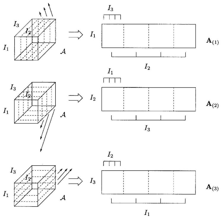
Unfolding the 3-mode tensor 𝔸 ∈ ℜ I1×I2×I3 to the matrices A(1) ∈ ℜ I1×(I2×I3), A(2) ∈ ℜ I2×(I3×I1) and A(3) ∈ ℜ I3×(I1×I2) (From (de Lathauwer et al., 2000))
The mode-n product of a matrix X ∈ ℜJn×In with a tensor 𝔸 ∈ ℜ I1×I2×…×In×…×IM is denoted by 𝔸 ×n 𝕏 and results in the tensor 𝔹 ∈ ℜ I1×I2×…×In−1×Jn×In+1×…×IM. It’s entries are bi1…in−1jnin+1…iM = Σinai1…in−1inin+1…iMxjnin. In terms of the flattened matrices, B(n) = XA(n).
Singular Value Decomposition (SVD) is a 2-mode tool commonly used in signal processing to reduce the dimensionality of the space and thereby reduce noise. SVD decomposes a matrix A into three other matrices, A = USVT, where the columns of U spans the row space of A and V spans the column space of A, while S is a diagonal matrix of singular values. By a similar extension, the N-mode SVD or Higher Order SVD (HOSVD) decomposes the multi-linear space spanned by tensor 𝔸 yielding a core tensor and orthonormal matrices spanning the vector spaces of each mode of the tensor, i.e:
| (6) |
The core tensor 𝕊 is analogous to the diagonal singular value matrix from traditional SVD and coordinates the interaction of matrices to produce the original tensor. Additionally, the Frobenious-norm of the sub-tensors of 𝕊 estimates the variance of the corresponding part of the original tensor. This could be used to reduce the feature space.
Dimensionality Reduction
Matrices Ui are orthonormal and their columns span the space of the flattened tensor T(i). The row vectors of Ui are the coefficients describing each dimension along mode i. 1 After conducting the HOSVD on a given image data, the dimensionality with respect to any mode can be reduced independently, unlike the PCA where dimensionality reduction is only based on the variance. By reducing the number of dimensions in one mode, we can selectively control how that mode explains the original space, and eliminate noise from each mode separately. The dimensions also are reduced by removing the last m-column vectors from the tensor flattened along the desired mode. The error after dimensionality reduction is bounded by the Frobenius norm of the corresponding hyper-planes in the core tensor.
3.4 Classification
Let C, L and K be discrete sets of tissue classes, training samples for each class and separation distances used in the computation of the 2-pcfs. As described in the preceding sections, for each distance ℓ ∈ K used in the 2-pcf computation, we extract a Q ×Q correlation matrix, where Q = 4 is the number of material phases in the tissue 2. We pack all these features, into a 5-mode tensor 𝔸 ∈ ℜ C×L×K×Q×Q. The first mode corresponds to the tissue classes, the second mode to the training instances, third mode to the separation distances, and fourth and fifth mode to vertex phases in the 2-pcf. This tensor is decomposed as:
| (7) |
The row vectors of are the coefficients describing each class and are used in classification.
Let 𝕏 K×Q×Q be the 2-pcf feature tensor for one training instance, with class c ∈ C and training instance number l ∈ L. Let be the jth row in the class matrix describing class j and be the lth row vector of the instance matrix, , describing instance l in the training data. Then by projecting into the decomposed space in Equation 7, we are able to reconstruct:
For a test feature tensor ℤK×Q×Q, the goal is now to find the class coefficients z1×C that will minimize its reconstruction error. Then, the reconstructed feature tensor is:
| (8) |
| (9) |
| (10) |
The best class coefficients are obtained by minimizing the following objective function:
| (11) |
The solution to this optimization problem turns out to be the solution to the linear system: A(l)x(l) = b(l) where
| (12) |
| (13) |
The best coefficient set z1×C is obtained by first selecting the training instance l that minimizes the error ε(l), and then computing the corresponding z1×C
4 Results
4.1 k-Nearest Neighbor classification using the 2, 3-pcf features
Here, we illustrate the working of the N-pcf features on very simple images with binary components. The N-pcfs were evaluated using three synthetic images with well-defined textures shown in Figure 6. The images consisted of two phases represented as black (phase 0) and white (phase 1) regions. The 2-pcfs were evaluated using line segments having varying lengths ℓ ∈ [1,25] pixel-units. Similarly, the 3-pcfs were evaluated using equilateral triangles with edge lengths ℓ ∈ [1,25] pixel units. The random sampling parameter was set as S = 500 with image windows Ω of size 40×40.
A k-nearest neighbor classifier (k=5) was used to identify the different texture types based on the observed 2-pcf and 3-pcf evaluations. This relatively simple classifier to study the feature space spanned by the N-pcfs. The training set for the classifier consisted of hundred regions randomly chosen from each texture type. For example, Image-1 presented four different textures. Therefore, the training set consisted of the 2-pcf and 3-pcf output on 400 regions. Classification was performed by considering the 2-pcf and the 3-pcf features independently. We present our results in Figure 7, Figure 8 and Figure 9. The algorithm generated region labels (along the column) are tabulated against the ground-truth labels (along the rows).
Fig. 7.

Classification results tabulated against the ground-truth on synthetic Image-1.
Fig. 8.

Classification results tabulated against the ground-truth on synthetic Image-2.
Fig. 9.

Classification results tabulated against the ground-truth on synthetic Image-3.
The accuracies for each texture class in Image-1 (Figure 7) was over 95% for both the 2-pcf and the 3-pcf features. At the same time, the rate of false identifications was low (<5%). The only notable exception was observed in class 3 (the vertical bars). The vertical bars fared poorly when evaluated using the 2-pcf feature set having a false positive rate of 9.1%. Most of the inaccuracies were confined to the boundaries since textures are not well-defined locally. Window patches at texture boundaries contain material from different tissues. Hence, the microstructure properties as captured by the N-pcf are representative of an intermediate material.
Image-2 suffered from higher inaccuracies but still maintained acceptable performance (>82%) for four of the five textures (Figure 8). The performance was relatively poor on the portion of the image with wide horizontal bars. The classification of the bars was often confused with that of the circles in the center of the image. The ambiguity occurred primarily at the boundaries. This was mainly a result of the features not being sufficiently discriminating at the scale of distances (ℓ) considered in the N-pcf features. As a consequence, this resulted in a classification accuracy ranging from 70% to 75% for the horizontal bars and false positive rates of 3.5% to 6%. It should be noted that the false positive rates for the circles in the center were higher than the normal 4% to 50%. The 3-pcf features performed much better than the 2-pcf. The high false positive rates are attributed to the same reasons of scale that was discussed above. This experiment shows that incorporating the right scale of N-pcf features is important in obtaining good accuracies while maintaining a low false positive rate.
Classification accuracy in Image-3 was within the range of 82.3 to 98.8% (Figure 9). Significantly, both the best and worst performance occurred while using the 2-pcf features. The thin concentric circles was identified with 98.8% accuracy while the wider concentric circles were identified with an accuracy of 82.3%. The lack of accuracy in the latter case was the result of identifying the wide concentric circles near the image boundary as vertical bars. This is well illustrated in Figure 10 where circles at large radii are similar to vertical bars. False positives were limited to the range of 0.5% and 21.6%. From this experiment, we observe that the 2-pcf features performed better as compared to the 3-pcf features which is a change from the trend observed in Image-2 wherein the 3-pcf features fared better.
Fig. 10.

Window patches from (a) texture class 2 and (b) texture class 4. Note the similarity in organization observed locally.
We now make the following observations about the performance of N-pcfs:
The textures regions are well-identified in the interiors. Ambiguity arise at the boundaries where the texture is not well-defined locally. The resolution depends on the window sizes Ω considered.
The correct scale of separation distances need to be considered. A wrong choice can lead to ambiguity across different texture classes.
While the 2-pcf and the 3-pcf output trends are correlated in most textures, some cases cause one of the measures to perform relatively better. Hence, it is useful to consider both the measures in any given image.
We now apply our segmentation framework to datasets acquired from phenotyping studies.
4.2 Mouse Placenta Phenotyping
A central issue in human cancer genetics requires the understanding of how the genotype change (e.g., gene mutations and knockout) affects phenotype (e.g., tissue morphology or animal behavior) and is valuable in the development of therapies to treat the diseases such as cancers. In common experimental conditions, the genotype change can be well controlled. Therefore, it is useful to quantitatively assess the corresponding phenotype change in the organism. Serial-section imaging (Fiala and Harris, 2002; Fiala, 2005; Wu et al., 2003; Wenzel et al., 2007) is one of the widely used phenotyping tools for making large-scale objective and automated analysis. We have applied our methods to two phenotyping studies that required a significant image analysis component. Image analysis is capable of providing viable biomarkers that can be used towards hypothesis generation,
We implemented our framework using the National Library of Medicine’s (NIH/ NLM) Insight Segmentation and Registration Toolkit (ITK) (Ibáñez and Schroeder, 2003) and the Visualization Toolkit (VTK) from Kitware Inc. The classified volumetric datasets are loaded into Kitware’s VolView volume visualization software to render the surface appropriately in both the case-studies. All our tasks were conducted on a 2.5GHz Pentium machines running Linux with 1GB main memory. The segmentation software processed a placenta slice completely in under 15 minutes. The mammary sections required 3–5 minutes owing to the use of a single 2-pcf feature.
Mouse placentas are composed of three distinct layers: the labyrinth, spongiotrophoblast, and glycogen layers as shown in Figure 1. The phenotyping experiments (Wu et al., 2003; Wenzel et al., 2007) required the quantification of morphological parameters related to the surface area, volume of the labyrinth and its interface with the spoongiotrophoblast layer. Hence, segmentation was deemed necessary and important.
The microscopic images are obtained from the standard histologically stained slides of both a wildtype and a mutated (Rb−) mouse placenta. The slides are collected by sectioning the wax fixed sample (placenta) at 3μm thickness. They are then digitized using a an Aperio Scanscope digitizer using a 20× magnification objective lens, producing effective magnification of 200× under which each image is of size between 500Mb and 1Gb. A total of more than 2,000 images are obtained (1,278 images for the wildtype and 786 images for the Rb−) with total file size of approximately 1.7 Terabytes.
4.3 Segmenting the Placental Tissue Layers
The first step consisted of identifying the tissue components. These were identified by modeling each component as a Gaussian distribution in the RGB color space. The modeling was performed by using the pixel training data gathered by the method described in Section 3. The 2 and 3-pcfs were evaluated at distances k ∈ [1,24] pixel units. A window size Ω of 51 × 51 dimensions was considered with sample size S = 1000. Since we were interested in comparing the utility of the N-pcf features with those of Haralick and Gabor features, classification was accomplished using the k-NN scheme (k = 5). Training data for the k-NN method was obtained as follows:
Training data
Image tissue patches of size 20 × 20 were generated and labeled as either labyrinth (Lab), spongiotrophoblast (SP), Glycogen (Glyc) or background (BG). A total of 2200 regions were selected from one image slide (800 for labyrinth, 800 for spongiotrophoblast, and 600 for the background). A total of 150 of these regions were used in training (50 for each region) and the rest is used for testing.
In Figure 11, we observe that the N-pcf s identified and labeled the labyrinth layer with an acceptable level of accuracy (≈ 96%) and a low false positive rate of 8.5–10.5%. The spongiotrophoblast was also classified with an accuracy of ≈ 96% and a false positive rate of 6–8%. The background material is identified with an accuracy of 99% to 100%. Glycogen was identified with an accuracy of only ≈ 50%. This was because the glycogen regions are smaller than the window size. They have almost the same microstructure characteristics as the labyrinth layer (refer to Figure 1). They are often difficult to perceive even to the human eye.
Fig. 11.

Comparison of the placenta segmentation output using four different feature sets. Acc: Accuracy. FP: False positives. Lab: Labyrinth layer. ST: Spongiotrophoblast. Glyc: Glycogen. BG: Background.
The Haralick features fared well on the labyrinth layer (95%) and the spongiotrophoblast (89%) but still presented slightly lower values than the N-pcf features. The Gabor features performed poorly only delivering a classification accuracy of 53% for the labyrinth and 80% for the spongiotrophoblast. The correlation functions meanwhile had the lowest rate of false positives of all of the features.
The better performance observed with the material science measures is a result of the component hierarchy used in the technique. While the Gabor and Haralick features are concerned with the luminance and co-occurrence of the image features, the newer measures are able to leverage the knowledge of the components and spatial distributions for better segmentations.
4.4 Comparing the k-Nearest Neighbor and the HOSVD Classification
In this section, we compare the performance of the simple k-NN and HOSVD classification scheme using the same labeled data that was prepared for the experiments in Section 4.3.
The resulting confusion matrix while using the k-NN classification on the N-pcf features is shown in Table 1. The k-NN classifier achieves above 90% in the labyrinth and the spongiotrophoblast regions. Notably, the k-NN algorithm performs very well in the spongiotrophoblast regions and achieves a classification accuracy of 96.8% but provides a high false positive rate of detection. Meanwhile, the HOSVD classifier without any dimensional reduction performs comparably to the k-NN classifier in Table 2. HOSVD improves the results to 94% in the labyrinth region but the accuracy decreases to 93.9% in the spongiotrophoblast areas. Nevertheless, the false positive rate of detection is consistently lower. The classification accuracy for the background is at 100% with 0% false positive rate for both the classifiers.
Table 1.
Confusion matrix entries for k-NN.
| Lab | SP | BG | Acc | |
|---|---|---|---|---|
|
| ||||
| Lab | 684 | 66 | 0 | 91.2% |
| SP | 61 | 726 | 0 | 96.8% |
| BG | 0 | 0 | 550 | 100% |
| FP | 8.1% | 8.3% | 0% | - |
Acc: Accuracy. FP: False positives. Lab: Labyrinth layer. ST: Spongiotrophoblast. BG: Background.
Table 2.
Confusion matrix entries for HOSVD classification with no dimensional reduction/35 dimensions/9 dimensions respectively.
| Lab | SP | BG | Acc | |
|---|---|---|---|---|
|
| ||||
| Lab | 705 | 717 | 617 | 45 | 33 | 47 | 0 | 94 | 95.6 | 92.3% |
| SP | 46 | 53 | 30 | 704 | 697 | 720 | 0 | 93.9 | 92.9 | 96.3% |
| BG | 0 | 0 | 550 | 100% |
| FP | 6 | 6.8 | 4.6% | 6 | 4 | 6.1% | 0% | - |
Acc: Accuracy. FP: False positives. Lab: Labyrinth layer. ST: Spongiotrophoblast. BG: Background.
Figure 12(a) shows the classification accuracies observed for all the four (4) classes when the dimension is reduced in the instance mode alone. The accuracy of detection sharply rises for the labyrinth layer when thirty-five (35) instances per class are considered. Meanwhile, the spongiotrophoblast detection is better while using around 9 samples. These numbers indicate that the variance of features describing spongiotrophoblast is mostly due to the noise, whereas the variance for the labyrinth is due to the variation in the data. We present the confusion matrices for both the cases in Table 2 (thirty-five(35) and nine (9) respectively).
Fig. 12.

Classification accuracies observed after dimensionality changes in (a) instances mode alone (b) distance mode alone.
Figure 12(b) shows the classification accuracies observed for all the four (4) classes when the dimension is reduced in the distance mode alone. The classification accuracy for the labyrinth layer decreases monotonically while the spongiotrophoblast remains unaffected. Finally, a choice that would serve both the labyrinth and spongiotrophoblast regions equally may be obtained by reducing the dimensionality by thirty (30) in instances mode and by two (2) in distance mode. This setup produces the confusion matrix shown in Table 3.
Table 3.
Confusion matrix for combined dimensional reduction using the HOSVD scheme.
| Lab | SP | BG | Acc | |
|---|---|---|---|---|
|
| ||||
| Lab | 692 | 58 | 0 | 92.30% |
| SP | 35 | 715 | 0 | 95.30% |
| BG | 0 | 0 | 550 | 100% |
| FP | 5.0 | 8.11 | 0 | |
Acc: Accuracy. FP: False positives. Lab: Labyrinth layer. ST: Spongiotrophoblast. Glyc: Glycogen. BG: Background.
To summarize our results:
The high accuracy in detection of the k-NN classifier are offset by the presence of high false positive rate.
The HOSVD scheme with dimensional reduction eliminates the modes that do not explain the tensor feature space and retains the significant ones. Hence, it helps in eliminating noise and cause better data separation.
Our results indicate that dimensionality reduction helps in providing the user more control in obtaining better segmentations on a particular region-of-interest as a trade-off against other regions.
In addition to the standard validation, we also measure the efficacy of the framework by inspecting the labyrinth-spongiotrophoblast interface.
4.5 Labyrinth-Spongiotrophoblast Interface Validation
Our framework processed four (4) pairs (eight in total) placenta datasets. Validation was carried out on three (3) placenta datasets. For each placenta, manual segmentation of the labyrinth layer was carried out on ten images that are evenly spaced throughout the image stack. In Figure 13, the automatically segmented labyrinth is overlaid on the manually segmented labyrinth tissue. For all the manually segmented images, the error is measured as the ratio of area difference between the two segmentations to the area of the manual labyrinth segmentation. Formally, let Im and Ia represent the manually and automatically segmented images. The boundary estimation error is defined as . For the three samples, the boundary estimation errors are 6.61.6%, 5.33.3%, and 16.77.4%. The errors are quite low for two of the three placentas given the fact that the validation has been conducted across the serial-section stack. As shown in Figure 13e and Figure 13f, the error can be attributed to two major reasons: (i) large window sizes in the N-pcf algorithm leads to a boundaries that suffer from a stair-case effect. (ii) discrepancy in assigning the large white areas on the boundary. The latter reason also explains why the automatic segmentation works less reliably in the case of the third placenta with the largest error (16.77.4%). The other two placenta (one wildtype and one mutant) with mean error less than 7% were then used for visualization. Figure 14 shows a placenta with marked up boundaries and the final segmentation result. Figure 15 shows the pair of selected wildtype and mutant placentas whose labyrinth layer is rendered as a binary volume using a simple transfer function.
Fig. 13.

Evaluation of the automatic segmentation algorithm. (a): The solid line is the manually marked boundary and the dashed line is the automatic segmentation result. (b), (c) and (d): examples of images with boundary estimation errors being 2.5%, 8.4% and 16.5%. (e) and (f): a larger view of the difference between manual segmentation (cyan) and automatic segmentation (purple).
5 Summary
In this paper, we described a tissue segmentation algorithm that is applicable in histology images obtained from serial-section microscopy. We estimated the packing and material component distribution locally using the N-point correlation functions. These functions are realized using suitable windowing and sampling strategies to provide tensor feature representations. Multi-linear properties of the tensor feature space are then extracted using a variant of the HOSVD algorithm. The algorithm allows the reduction of the dimensionality of the tensor feature space with respect to the significant modes thereby achieving robust classification. Our methods have been applied in a mouse model phenotyping study requiring the segmentation of the labyrinth tissue layer in the placenta. The classifier performance and the final segmentation output was validated extensively using manual ground-truth. In future, we would like to extend the feature set with additional spatial proximity measures that efficiently represent the microstructure. These measures would address some of the challenges in the segmentation of large histology images. Additionally, we would like to investigate possible enhancements in performance that may be obtained from utilizing efficient structures such as the quadtrees and kd-trees on large images.
Footnotes
They are similar to the coefficients extracted from PCA but there exist different sets of coefficients for each mode in a typical HOSVD analysis. Please refer to Vasilescu and Terzopoulos (200) for details.
nuclei, RBCs, cytoplasm and background
Publisher's Disclaimer: This is a PDF file of an unedited manuscript that has been accepted for publication. As a service to our customers we are providing this early version of the manuscript. The manuscript will undergo copyediting, typesetting, and review of the resulting proof before it is published in its final citable form. Please note that during the production process errors may be discovered which could affect the content, and all legal disclaimers that apply to the journal pertain.
Contributor Information
Kishore Mosaliganti, Email: mosaligk@cse.ohio-state.edu.
Firdaus Janoos, Email: janoos@cse.ohio-state.edu.
Okan Irfanoglu, Email: irfanogl@cse.ohio-state.edu.
Randall Ridgway, Email: ridgwayr@cse.ohio-state.edu.
Raghu Machiraju, Email: raghu@cse.ohio-state.edu.
Kun Huang, Email: khuang@bmi.ohio-state.edu.
Joel Saltz, Email: joel.saltz@osumc.edu.
Gustavo Leone, Email: gustavo.leone@osumc.edu.
Michael Ostrowski, Email: michael.ostrowski@osumc.edu.
References
- Aste T, Weaire D. The Pursuit of Perfect Packing. Institute of Physics Publishing; 2000. [Google Scholar]
- Babu G, Feigelson E. Stochastic problems in physics and astronomy. Reviews of Modern Physics. 1943;15:1–89. [Google Scholar]
- Beucher S. The watershed transformation applied to image segmentation. Conference on Signal and Image Processing in Microscopy and Microanalysis; 1991. pp. 299–314. [Google Scholar]
- Braumann U, Kuska J, Einenkel J, Horn L, Löffler M, Höckel M. Three-dimensional reconstruction and quantification of cervical carcinoma invasion fronts from histological serial sections. IEEE Transactions in Medical Imaging. 2005;24(10):5–7. doi: 10.1109/42.929614. [DOI] [PubMed] [Google Scholar]
- Caselles V, Kimmel R, Sapiro G. Geodesic active contours. International Journal on Computer Vision. 1997;22(1):61–97. [Google Scholar]
- Chandrasekhar S. Spatial point processes in astronomy. Journal of Statistical Planning and Inference. 1996;50(3):311–326. [Google Scholar]
- Chen T, Metaxas D. A hybrid framework for 3d medical image segmentation. Medical Image Analysis. 2005;9:547–565. doi: 10.1016/j.media.2005.04.004. [DOI] [PubMed] [Google Scholar]
- Cooper L, Huang K, Sharma A, Mosaliganti K, Pan T. Registration vs. reconstruction: Building 3-d models from 2-d microscopy images. Proceedings of Workshop on Multiscale Biological Imaging, Data Mining and Informatics; 2006. pp. 57–58. [Google Scholar]
- de Lathauwer L, de Moor B, Vandewalle J. A multilinear singular value decomposition. SIAM Journal of Matrix Analysis and Applications. 2000;21(4):1253–1278. [Google Scholar]
- Fernandez-Gonzalez R, Deschamps T, Idica A, Malladi R, de Solorzano C. Automatic segmentation of histological structures in mammary gland tissue sections. Biomedical Optics. 2004;9(3):444–453. doi: 10.1117/1.1699011. [DOI] [PubMed] [Google Scholar]
- Fiala J. Reconstruct: a free editor for serial section microscopy. Journal of Microscopy. 2005;218:52–61. doi: 10.1111/j.1365-2818.2005.01466.x. [DOI] [PubMed] [Google Scholar]
- Fiala J, Harris K. Computer-based alignment and reconstruction of serial sections. Microscopy and Analysis. 2002;52:5–7. [Google Scholar]
- Fridman Y, Pizer S, Aylward S, Bullitt E. Extracting branching tubular object geometry via cores. Medical Image Analysis. 2004;8:169–176. doi: 10.1016/j.media.2004.06.017. [DOI] [PubMed] [Google Scholar]
- Gokhale A. Experimental measurements and interpretation of microstructural n-point correlation functions. Microscopy and Microanalysis. 2004;10:736–737. [Google Scholar]
- Gokhale A, Tewari A, Garmestani H. Constraints on microstructural two-point correlation functions. Scripta Materialia. 2005;53:989–993. [Google Scholar]
- Haralick R, Shanmugam K, Dinstein I. Textural features for image classification. IEEE Transactions on Systems, Man and Cybernetics. 1973:610–621. [Google Scholar]
- Huang A, Nielson G, Razdan A, Farin G, Baluch D, Capco D. Thin structure segmentation and visualization in three-dimensional biomedical images: A shape-based approach. IEEE Transactions in Visualization and Computer Graphics. 2006;12(1):93–102. doi: 10.1109/TVCG.2006.15. [DOI] [PubMed] [Google Scholar]
- Huang K, Murphy RF. Automated classification of subcellular patterns in multicell images without segmentation into single cells. IEEE International Symposium of Biomedical Imaging (ISBI 2004); 2004. pp. 1139–1142. [Google Scholar]
- Ibáñez L, Schroeder W. The ITK Software Guide. Kitware, Inc; 2003. [Google Scholar]
- Janoos F, Irfanoglu O, Mosaliganti K, Machiraju R, Huang K, Wenzel P, deBruin A, Leone G. Multi-resolution image segmentation using the 2-point correlation functions. IEEE International Symposium of Biomedical Imaging.2007. [Google Scholar]
- Jeong Y, Radke R. Reslicing axially sampled 3d shapes using elliptic fourier descriptors. Medical Image Analysis. 2006;11:197–206. doi: 10.1016/j.media.2006.12.003. [DOI] [PubMed] [Google Scholar]
- Levenson R, Hoyt C. Spectral imaging and microscopy. American Laboratory. 2000;32(1):26–34. [Google Scholar]
- Malladi R, Sethian JA, Vermuri BC. Shape modeling with front propagation: A level set approach. IEEE Tranactions on Pattern Analysis and Machine Intelligence. 1995;17(2):158–174. [Google Scholar]
- Mosaliganti K, Machiraju R, Heverhagen J, Saltz J, Knopp M. Exploratory segmentation using geometric tessellations. Proceedings of 10th International Fall Workshop on Vision, Modeling and Visualization; 2005. pp. 1–8. [Google Scholar]
- Ohtake T, Kimijima I, Fukushima T, Yasuda H, Sekikawa M, Takenoshita S, Abe R. Computer-assisted complete three-dimensional reconstruction of the mammary ductal/lobular systems. Cancer. 2001;91(12):2263–2314. doi: 10.1002/1097-0142(20010615)91:12<2263::aid-cncr1257>3.0.co;2-5. [DOI] [PubMed] [Google Scholar]
- Pan T, Huang K. Virtual mouse placenta: Tissue layer segmentation. Proceedings of the 27th Annual International Conference of the IEEE Engineering in Medicine and Biology Society; 2005. [DOI] [PubMed] [Google Scholar]
- Ridgway R, Irfanoglu O, Machiraju R, Huang K. Image segmentation with tensor-based classification of N-point correlation functions. MICCAI Workshop on Medical Image Analysis with Applications in Biology; 2006. [DOI] [PMC free article] [PubMed] [Google Scholar]
- Saheli G, Garmestani H, Adams B. Microstructure design of a two phase composite using two-point correlation functions. Computer-Aided Materials Design. 2004;11(2–3):103–115. [Google Scholar]
- Sharp R, Ridgway R, Mosaliganti K, Wenzel P, Pan T, Bruin A, Machiraju R, Huang K, Leone G, Saltz J. Volume rendering phenotype differences in mouse placenta microscopy data. Special Issue on Anatomic Rendering and Visualization, Computing in Science and Engineering. 2007;9(1):38–47. [Google Scholar]
- Singh H, Mao Y, Sreeranganathan A, Gokhale A. Application of digital image processing for implementation of complex realistic particle shapes/morphologies in computer simulated heterogeneous microstructures. Modeling and Simulation in Material Science and Engineering. 2006;14:351–363. [Google Scholar]
- Sloane B, Gillies R, Mohla S, Sogn J, Menkens A, Sullivan D. I2 imaging: Cancer biology and the tumor microenvironment. Cancer Research. 2006;66(23):11097–11101. doi: 10.1158/0008-5472.CAN-06-3102. [DOI] [PubMed] [Google Scholar]
- Stephens D, Allan V. Light microscopy techniques for live cell imaging. Science. 2003;300(5616):82–86. doi: 10.1126/science.1082160. [DOI] [PubMed] [Google Scholar]
- Stoyan D, Kendall S, Mecke J. Stochastic geometry and its applications. John Wiley and Sons; New York: 1985. [Google Scholar]
- Streicher J, Donat M, Strauss B, Sporle R, Schughart K, Müller G. Computer-based three-dimensional visualization of developmental gene expression. Nature Genetics. 2000;25:147–152. doi: 10.1038/75989. [DOI] [PubMed] [Google Scholar]
- Sundararaghavan V, Zabaras N. Classification and reconstruction of three-dimensional microstructures using support vector machines. Computational Materials Science. 2005;32:223–239. [Google Scholar]
- Torquato S. Random Heterogenous Material. Springer Verlag; 2004. [Google Scholar]
- Vasilescu MAO, Terzopoulos D. Multilinear subspace analysis for image ensembles. Proc Computer Vision and Pattern Recognition Conf (CVPR ’03) 2:93–99. 200. [Google Scholar]
- Wenzel P, Wu L, deBruin A, Chen W, Dureska G, Sites E, Pan T, Sharma A, Huang K, Ridgway R, Mosaliganti K, Sharp R, Machiraju R, Saltz J, Yamamoto H, Cross J, Robinson M, Leone G. Rb is critical in a mammalian tissue stem cell population. Genes and Development. 2007;21(1):85–97. doi: 10.1101/gad.1485307. [DOI] [PMC free article] [PubMed] [Google Scholar]
- Wu L, de Bruin A, Saavedra HI, Starovic M, Trimboli A, Yang Y, Opavska J, Wilson P, Thompson J, Ostrowski M, Rosol T, Woollett L, Weinstein M, Cross J, Robinson M, Leone G. Extra-embryonic function of Rb is essential for embryonic development and viability. Journal of Nature. 2003;421:942–947. doi: 10.1038/nature01417. [DOI] [PubMed] [Google Scholar]
- Zou G, Wu H. Nearest-neighbor distribution of interacting biological entities. Theoretical Biology. 1995;172(4):347–353. doi: 10.1006/jtbi.1995.0032. [DOI] [PubMed] [Google Scholar]