Mapping landscape friction to locate isolated tsetse populations that are candidates for elimination

Significance

Tsetse flies transmit human and animal trypanosomoses in Africa, respectively a neglected disease (sleeping sickness) and the most important constraint to cattle production in infested countries (nagana), and they are the target of the Pan African Tsetse and Trypanosomoses Eradication Campaign (PATTEC). Here, we used genetic distances and remotely sensed environmental data to identify natural barriers to tsetse dispersal and potentially isolated tsetse populations for targeting elimination programs. The method can be used to prioritize intervention areas within the PATTEC initiative and it is applicable to the control campaigns of other vector and pest species, as well as to the conservation of endangered species in fragmented habitats.

Abstract

Tsetse flies are the cyclical vectors of deadly human and animal trypanosomes in sub-Saharan Africa. Tsetse control is a key component for the integrated management of both plagues, but local eradication successes have been limited to less than 2% of the infested area. This is attributed to either resurgence of residual populations that were omitted from the eradication campaign or reinvasion from neighboring infested areas. Here we focused on Glossina palpalis gambiensis, a riverine tsetse species representing the main vector of trypanosomoses in West Africa. We mapped landscape resistance to tsetse genetic flow, hereafter referred to as friction, to identify natural barriers that isolate tsetse populations. For this purpose, we fitted a statistical model of the genetic distance between 37 tsetse populations sampled in the region, using a set of remotely sensed environmental data as predictors. The least-cost path between these populations was then estimated using the predicted friction map. The method enabled us to avoid the subjectivity inherent in the expert-based weighting of environmental parameters. Finally, we identified potentially isolated clusters of G. p. gambiensis habitat based on a species distribution model and ranked them according to their predicted genetic distance to the main tsetse population. The methodology presented here will inform the choice on the most appropriate intervention strategies to be implemented against tsetse flies in different parts of Africa. It can also be used to control other pests and to support conservation of endangered species.

Tsetse flies transmit trypanosomes, the causative agents of sleeping sickness (human African trypanosomosis, HAT) and nagana (African animal trypanosomosis, AAT). Through increased disease surveillance and treatment, the number of HAT cases has substantially declined in the last 15 y (1). However, the elimination of HAT as a public health problem also requires effective vector management (1). AAT continues to represent the greatest animal-health constraint to improved livestock production in sub-Saharan Africa, causing enormous economic losses (e.g., milk and meat production) (2). AAT also constrains the integration of crop farming and livestock keeping, a crucial component for the development of sustainable agricultural systems (3). Indeed, AAT affects animal draft power, and consequently crop production. Also, keeping less productive trypanotolerant cattle breeds pushes farmers to increase herd sizes with such negative environmental impacts as overgrazing. As an example, in the Niayes area of Senegal, it was estimated that the eradication of tsetse flies would allow cattle sales to triple whereas herd sizes would decrease by 45% (4).

The Challenges of Tsetse Elimination

Despite substantial efforts for over a century, deliberate efforts to reduce the vast tsetse belt have had very limited success (5). In past decades, spraying of residual insecticides was effective in certain areas, but this technique is no longer acceptable on environmental grounds. More recently, two environmentally friendly campaigns achieved sustained elimination by targeting isolated tsetse populations as a whole (6, 7). It is therefore useful to identify islands (8) or ecological islands (9) where isolated tsetse populations could be eradicated without risk of reinvasion. Although attempts have been made to identify isolated tsetse populations* (10, 11), a well-defined and reproducible method that can be applied on a regional scale is still lacking.

Landscape Friction, Genetics, and Dispersal

Given the high costs of field sampling, and the difficulty in accessing some of the sites, it is impossible to adopt a population genomic approach based on a systematic sampling of tsetse populations. Modeling landscape friction would thus represent a major advance to inform the prioritizing of tsetse elimination campaigns, with promising applications at the continent level.

Landscape friction, or its inverse, landscape permeability, modulates how animal species can move in the environment. In the field of landscape genetics, friction is modeled to (i) identify landscape and environmental features that constrain genetic connectivity, (ii) elucidate the ecological processes that influence spatial genetic structure, mainly to inform resources management and conservation, and (iii) predict how future landscape changes might influence genetic connectivity (12). Landscape friction has been studied in a number of species, with insects only represented in fewer than 10% of the studies (13). For example, studying friction allowed researchers to demonstrate that the rate of water loss plays a key role in the movement of a terrestrial woodland salamander, but also that models of habitat suitability or abundance may not be adequate proxies for gene flow (14).

In tsetse, consistent estimates of Glossina palpalis gambiensis dispersal at the microscale were obtained using direct methods (mark–release–recapture) as well as indirect ones (genetic isolation by distance) (15). Although a strong isolation by distance was observed in this species, tsetse populations separated by only 15 km of rice plantations (16) were found to be more isolated than others separated by 100 km of gallery forest (15). In other words, for this riverine tsetse species the friction of riparian woody vegetation is significantly lower than that of rice plantations. Despite its potential usefulness, no friction map is available for tsetse flies at any scale, and our attempts to generate one for G. p. gambiensis by using global land-cover maps and expert-based cost parameters (13) proved ineffective. By contrast, we built a friction map by iterating linear regression models of genetic distance and environmental parameters and by determining least-cost dispersal paths. The novelty of our approach is to relax the need for expert opinion and to rely fully on the genetic distance for an evidence-based mapping of landscape connectivity and for the identification of the most likely dispersal paths. We subsequently combined the genetics-based analysis of friction with a tsetse distribution model built using a fully different dataset, thus considering that habitat suitability and connectivity might not be influenced by the same environmental factors (14). The end result is a reproducible methodology that enabled us to locate potentially isolated tsetse populations that might be considered as targets in eradication programs.

Results and Discussion

Effect of Environmental Factors on Genetic Distance.

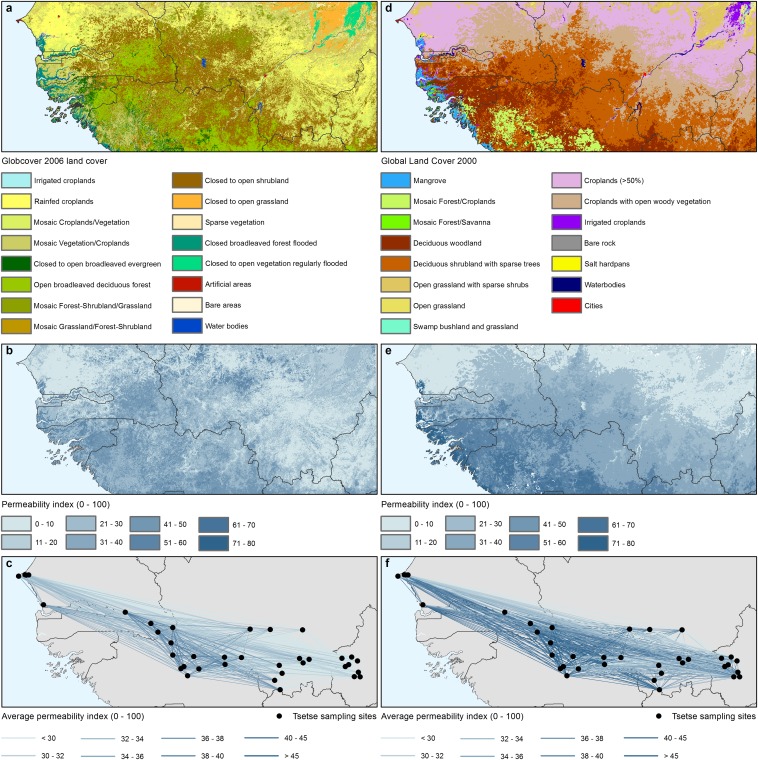
Using a linear regression model, we estimated the relationship between genetic distance [Cavalli-Sforza and Edwards’ chord distance (CSE), i.e., the response] and a set of environmental factors (the explanatory variables), the latter being initially calculated along the direct paths connecting tsetse populations pairwise (Figs. S1–S3). Expert-based permeability/friction scores had been first explored using global land-cover datasets (Global Land Cover 2000 and Globcover 2006). No significant correlation was found with genetic distance (Fig. S1, Table S1, and Details on the Genetic Analysis).

Fig. S1.

Expert-based knowledge to derive landscape permeability from landcover. (A) Globcover 2006 land cover (56). (B) Permeability index for G. p. gambiensis as derived from Globcover 2006. (C) Average permeability index between entomological sampling sites as derived from Globcover 2006. (D) GLC2000 land cover (55). (E) Permeability index for G. p. gambiensis as derived from GLC2000. (F) Average permeability index between entomological sampling sites. See Details on the Genetic Analysis and Table S2 for a description of the expert-based permeability scores for the different land-cover categories.

Fig. S3.

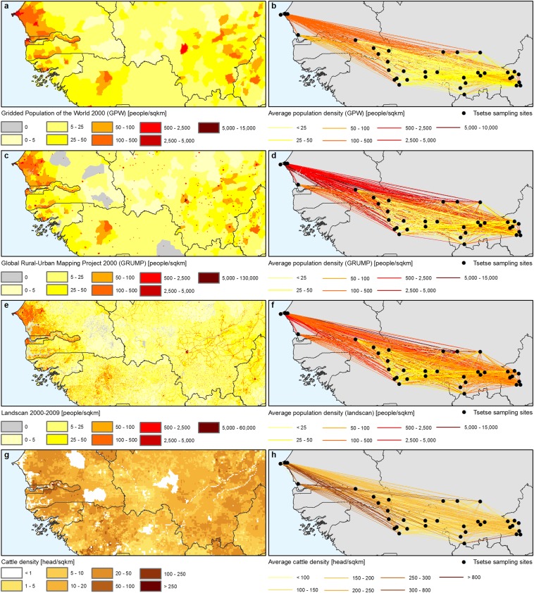
Population density datasets for genetics. (A) Human population density for the year 2000 (GPW) (59). (B) Average population density (GPW) between entomological sampling sites. (C) Human population density for the year 2000 (GRUMP) (60). (D) Average population density (GRUMP) between entomological sampling sites. (E) Human population density for the years 2000–2009 (Landscan) (61). (F) Average population density (Landscan) between entomological sampling sites. (G) Cattle density for the year 2000 (62). (H) Average cattle density between entomological sampling sites.

Table S1.

Permeability scores for the land-cover classes present in the study areas

Dataset	Land-cover class	Permeability
GLC2000	Mangrove	80
	Mosaic forest/croplands	70
	Mosaic forest/savanna	80
	Deciduous woodland	60
	Deciduous shrubland with sparse trees	40
	Open grassland with sparse shrubs	20
	Open grassland	10
	Swamp bushland and grassland	30
	Croplands (>50%)	10
	Croplands with open woody vegetation	25
	Irrigated croplands	5
	Bare rock	0
	Salt hardpans	0
	Waterbodies	0
	Cities	0
Globcover 2006	Postflooding or irrigated croplands (or aquatic)	5
	Rainfed croplands	5
	Mosaic cropland (50–70%)/vegetation (grassland/shrubland/forest) (20–50%)	10
	Mosaic vegetation (grassland/shrubland/forest) (50–70%)/cropland (20–50%)	30
	Closed to open (>15%) broadleaved evergreen or semideciduous forest (>5 m)	60
	Open (15–40%) broadleaved deciduous forest/woodland (>5 m)	50
	Mosaic forest or shrubland (50–70%)/grassland (20–50%)	60
	Mosaic grassland (50–70%)/forest or shrubland (20–50%)	30
	Closed to open (>15%) (broadleaved or needle-leaved, evergreen, or deciduous) shrubland (<5 m)	30
	Closed to open (>15%) herbaceous vegetation (grassland, savannas, or lichens/mosses)	15
	Sparse (<15%) vegetation	5
	Closed (>40%) broadleaved forest or shrubland permanently flooded, saline or brackish water	60
	Artificial surfaces and associated areas (urban areas >50%)	0
	Bare areas	0
	Water bodies	0

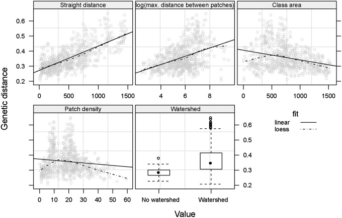
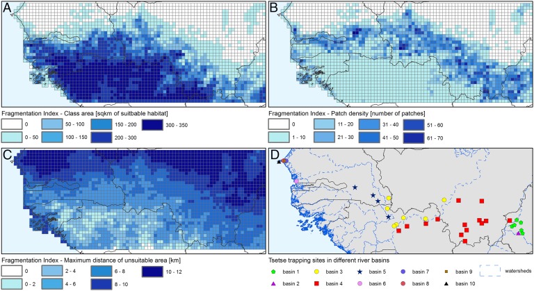
In the regression model, the main variables influencing genetic distance were (i) the geographic distance, (ii) being located within the same river basin, and (iii) three different metrics of habitat fragmentation, namely the patch density [number of habitat patches (i.e., tree cover >20%) within the 0.2° pixels where landscape friction is modeled], the class area [number of habitat pixels (500 × 500 m)]), and the maximum distance between habitat patches (Fig. 1). The findings were consistent with existing knowledge of G. p. gambiensis ecology. For example, isolation by distance is well known, as is the effect of watersheds on genetic distance, even if the latter does not lead to complete isolation (Fig. S4) (11). Human encroachment on tsetse habitat explains the positive effect of habitat fragmentation on genetic distance: The further apart the habitat patches, the more difficult for tsetse to disperse (Fig. 2) (17).

Fig. 1.

Shape and amplitude of the relationships between genetic distance, great-circle distance and environmental variables. CSE was calculated between pairs of G. p. gambiensis populations (37 sampling sites listed in Table S1) and environmental variables are here extracted along the straight paths.

Fig. S4.

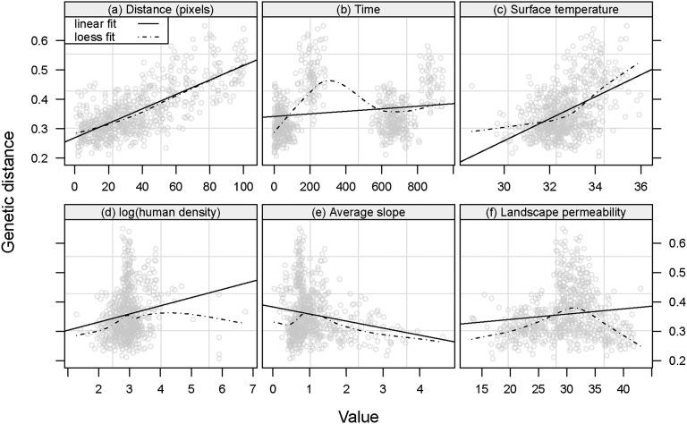
Relationship between the genetic distance and various environmental factors. The panels present the CSE (24) as a function of seven variables. (A) Number of pixels along each line connecting pairwise the entomological sampling sites along the direct paths. (B) Time between sampling dates (days). (C) Daytime land surface temperature (degrees Celsius). (D) Logarithm of human density (inhabitants per square kilometer). (E) Average slope. (F) Permeability index derived from Globcover 2006.

Fig. 2.

Landscape fragmentation and river basins. Landscape fragmentation of G. p. gambiensis habitat based on a tree cover threshold of 20% (year 2000) (44) and related linear fragmentation indices. (A) Patch area. (B) Patch density. (C) Maximum distance of unsuitable area (or maximum distance between patches). (D) Locations of the tsetse sampling sites grouped by river basin (45).

Identification of Tsetse Dispersal Paths.

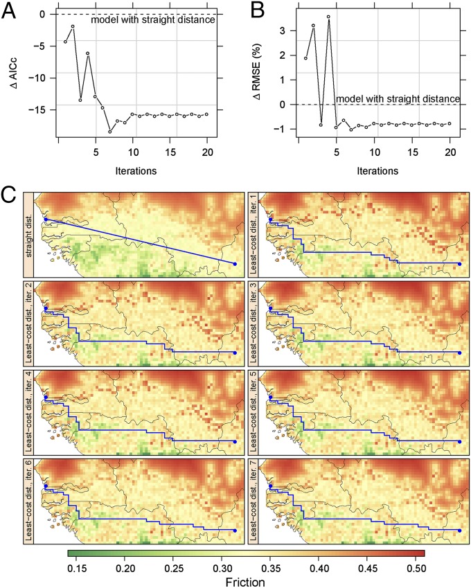
Direct lines connecting the sampled tsetse populations were initially used to model the genetic distance against the environmental variables, thereby generating the initial friction map. Subsequently, the average values for the environmental variables were recalculated along the least-cost paths based on the initial friction map (Fig. 3). To this end, a transition matrix was computed from the friction map. To define the connectedness between adjacent pixels, we used Rooks’ distance as a neighborhood function, in which a given pixel is considered to be connected to the four adjacent pixels. Then, the least-cost paths between origin and destination points were calculated, minimizing the mean values of friction for the pixels crossed by the path. The new set of values of explanatory variables extracted along this least-cost path was used to refit the regression model. This procedure was repeated 20 times, and models fitted at each iteration were compared with the Akaike information criterion corrected for small sample size (AICc): The smaller, the better. A large reduction of AICc was observed between the initial model based on direct lines and the AICc-best model based on least-cost paths: ∆ AICc = 18 (Fig. 3A). Thus, the regression model based on least-cost paths (seventh iteration) was much more plausible than the initial one. It also minimized the root mean squared error (Fig. 3B).

Fig. 3.

Least-cost distance vs. straight distance. (A) Observed changes in Akaike information criterion with small-sample size correction (AICc) and (B) rmse when replacing straight distance with least-cost distance computed from the friction raster, and iterating the process (x axis). (C) Changes in landscape genetic friction (colored map) and in least-cost distance (blue line) between two tsetse populations over the first seven iterations.

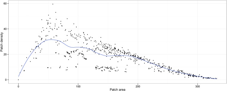
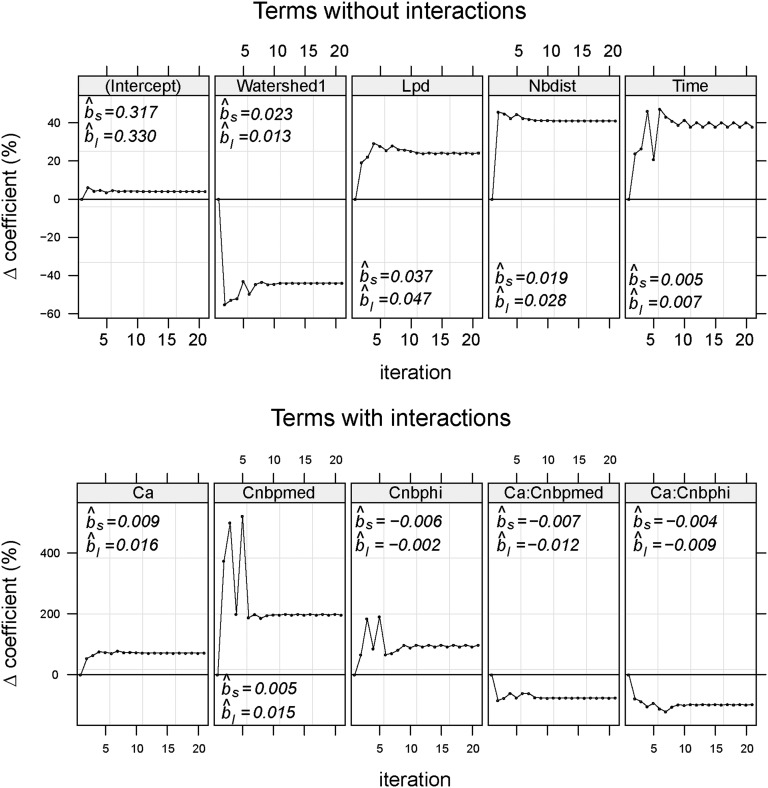
Apart from the time between sampling events and the geographical distance, all variables retained in the AICc-best model (coefficients in Table S2) were describing landscape connectivity (i.e., landscape fragmentation metrics and the presence of a watershed) (Fig. 2). There was a nonlinear relationship between the density and area of habitat patches, as expected in a fragmentation process (Fig. S5). Moreover, the interaction term between these two variables was retained in the final model. The variables informing on the composition and shape of the fragmented landscape and the geographic distance became more important in the final model, whereas the importance of watersheds and interactions was reduced (Fig. S6).

Table S2.

Fixed-effect coefficients for the AICc-best GLS model of genetic distance

Parameter	Value	SE	t value	P value
(Intercept)	0.3307	0.0098	33.9	< 10−3
Ca	0.0160	0.0031	5.1	< 10−3
Cnbpmed	0.0141	0.0090	1.6	0.118
Cnbphi	−0.0010	0.0092	−0.1	0.909
Interflu1	0.0132	0.0067	2.0	0.050
Lpd	0.0463	0.0067	6.9	< 10−3
Nbdist	0.0275	0.0018	15.0	< 10−3
Time	0.0069	0.0028	2.5	0.013
Ca:Cnbpmed	−0.0128	0.0022	−5.9	< 10−3
Ca:Cnbphi	−0.0085	0.0025	−3.4	< 10−3

Ca, class area (number of pixels (500 m × 500 m) of suitable habitat in the 0.2° pixels where the landscape friction prediction is done; Cnbpmed and Cnbphi, medium and high categories of patch density, respectively [i.e., the number of pixels (500 m × 500 m) of suitable habitat within the 0.2° pixels where the landscape friction prediction is done]; Interflu1, presence of an interfluve; Lpd, logarithm of the maximal distance between patches of suitable habitat; Nbdist, distance along the least-cost paths; Time, time interval between sampling dates. Interactions are denoted with a colon.

Fig. S5.

Nonlinear relationship between patch density and class area. This strongly skewed shape corresponds to a classical fragmentation process progressing from right to left (loess-smooth trend presented as a blue line). Points represent estimates for all of the pairs of sampled populations of G. p. gambiensis.

Fig. S6.

Relative changes in model coefficients of genetic distance between tsetse populations when replacing straight distance with least-cost distance. ${\widehat{b}}_s$, estimated coefficient for straight-distance regression model; ${\widehat{b}}_l$, estimated coefficient for least-cost distance regression model.

The use of least-cost distance confirmed the significant impact of time between sampling dates on the genetic distance (Table S2) (16). More importantly, it revealed the importance of landscape features related to functional connectivity (Table S2). The iterative, least-cost-based analysis also improved the mapping of ecological barriers to tsetse dispersal, with a more contrasted picture of friction (Fig. 3C).

Distribution of G. p. gambiensis in the Study Area and Combination with Landscape Friction.

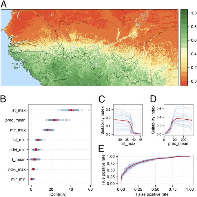
The habitat suitability for G. p. gambiensis was estimated using a maximum entropy (MaxEnt) model and mapped independently from landscape friction. Tsetse habitat was positively associated to vegetation activity [i.e., normalized difference vegetation index (NDVI)], average precipitations, and humidity. Conversely, high values for temperature-related variables [land surface temperature (LST) and air temperature] led to a low suitability index. Fig. 4 presents the respective contributions and response curves for the different variables, the most important being maximum LST and average precipitation. The predictive power of the MaxEnt model was high, with an area under the curve of 0.84 (Fig. 4). Moreover, the precision of MaxEnt predictions was the highest in the areas of interest (northern limit of the tsetse belt), which was also the most intensively sampled area (Fig. S7). Finally, we used a density-based clustering algorithm applied to the MaxEnt output to identify eight clusters of suitable habitat located at least 10 km apart from the main tsetse habitat.

Fig. 4.

Distribution of G. p. gambiensis in West Africa. (A) Mean habitat suitability index predicted by a MaxEnt model. The index varies between 0 (less suitable, red scale) and 1 (highly suitable, green scale). (B) Contribution of variables to the suitability index by decreasing importance (95% confidence interval in red and individual values in blue). lst_max, maximum land surface temperature (MODIS); lst_min, minimum land surface temperature (MODIS); mir_max, maximum mid-infrared reflectance (MODIS); mir_min, minimum mid-infrared reflectance; ndvi_max, maximum normalized difference vegetation index (MODIS); ndvi_min, minimum normalized difference vegetation index (MODIS); prec_mean, mean yearly rainfalls (WorldClim grid); t_mean, mean annual temperature (WorldClim grid). (C and D) Response curves of the most contributing variables (lst_max and prec_mean, respectively). (E) Area under the curve for the average MaxEnt model (in red) and the 45 submodels (in blue) (see Details on the MaxEnt Model for details).

Fig. S7.

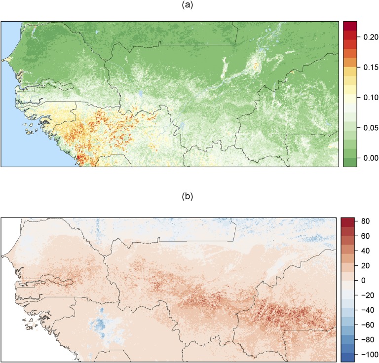
Uncertainty of MaxEnt predictions. (A) SD of suitability index across all 45 fitted models. (B) Multivariate environmental similarity surface plot for the environmental and occurrence data. Area in blue indicate zones of novel environmental condition where extrapolation should be interpreted with caution, whereas areas in red are the ones were the condition on the training data allow us to extrapolate accurately (in the training data range).

Model Predictions and Consequences for Tsetse Control.

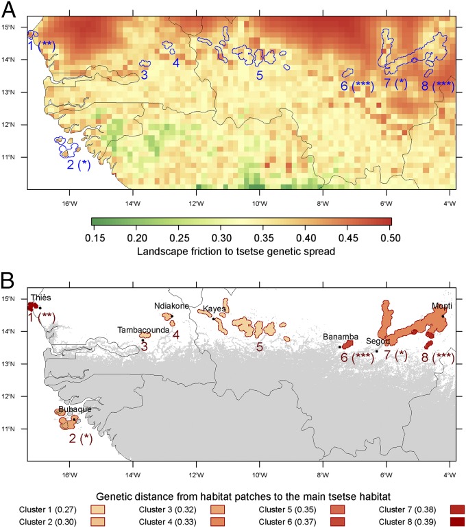
Fig. 5 presents the eight potentially isolated clusters of tsetse habitat located at the northern distribution limit of the G. p. gambiensis belt in West Africa. The population with the highest predicted genetic distance from the main tsetse belt (P = 0.003) was close to Thiès (Senegal). It is also the target of an ongoing eradication campaign. For this population, genetic isolation was confirmed by independent morphometric and genetic studies (9). Two other clusters (6 and 8) with similar genetic distances from the tsetse belt seemed to be isolated (P = 0.001) and therefore represent interesting potential targets for elimination efforts. Finally, two other clusters could be isolated (2 and 7, P < 0.05). Interestingly, the situation in cluster 2 (Bijagos Islands in Guinea Bissau) is reminiscent of the Loos Islands in Guinea (not visible in Fig. 5). The tsetse populations in the Loos Islands were recently targeted by an elimination program following the demonstration of their isolation (8).

Fig. 5.

Isolated patches of suitable habitat for G. p. gambiensis. (A) Landscape friction is the colored background, and habitat patches are delimited with blue contours. (B) The main tsetse belt predicted by MaxEnt for a sensitivity of 0.90 is in gray and habitat patches are shown as filled, red shapes. Contours and shapes of isolated patches were defined as 5-km radius buffers around pixels of habitat patches. The genetic distance of these patches to the main tsetse belt (reddish scale) was predicted by the AICc-best regression model along least-cost paths. Asterisks after cluster numbers represent the P values for the friction between the patches and the general habitat: (***) P = 10⁻³, (**) 10⁻³ ≤ P < 10⁻², (*) 10⁻² ≤ P < 5 10⁻².

The present study provides information on potential targets for tsetse elimination across a vast area. However, should one of these populations be selected for an elimination program, more comprehensive local studies would be needed, both to characterize the exact extent and connectivity of the infested area and to confirm its genetic isolation. These studies should include systematic sampling of suitable habitats (18) and an independent genetic analysis involving the target population and those closest to it (9).

Future Prospects.

Microsatellite genetic markers are available for the most important tsetse species: Glossina fuscipes, Glossina morsitans, Glossina pallidipes, and Glossina tachinoides. Furthermore, the recent sequencing of the full genome of G. morsitans offers new prospects for either additional microsatellite markers or other markers such as single-nucleotide polymorphisms (19). Applying the methodology described in this study to other tsetse species and regions would provide decision makers with crucial information on where control or eradication programs might be more appropriate. Friction maps might also help in those situations where the populations targeted for eradication are not isolated (e.g., the Mouhoun River in Burkina Faso and northwestern Ghana). In fact, artificial barriers to reinvasion such as traps impregnated with insecticides (6) would be more effective if deployed in high-friction areas. The use of such artificial barriers might therefore enable sequential eradication programs, by dividing the target populations into partially isolated subunits (20). Furthermore, in those areas exposed to strong reinvasion pressure, landscape friction analysis could guide the adoption of alternative strategies (e.g., reduction of tsetse densities below the threshold of disease transmission), thus preventing major economic losses due to unsuccessful eradication attempts.

Finally, identifying natural barriers to dispersal and quantifying their environmental determinants might help to manage other pests, or conversely it could be used to improve the conservation of endangered species occurring as metapopulations (21). Indeed, locating genetic corridors across high-friction landscapes is becoming crucial for the conservation of natural populations in a context of increasing fragmentation of ecosystems (12).

Details on the Genetic Analysis

Genotyping Procedure.

In each tube containing three tsetse legs, 200 µL of 5% Chelex chelating resin was added. After incubation at 56 °C for 1 h, DNA was denatured at 95 °C for 30 min. The tubes were then centrifuged at 12,000 × g for 2 min and frozen for later analysis. The PCR reactions were carried out in a thermocycler (MJ Research) in 10-mL final volume, using 1 µL of the supernatant from the extraction step. After PCR amplification, allele bands were resolved on a 4300 DNA Analysis System (LI-COR) after migration on 96-lane reloadable 6.5% denaturing polyacrylamide gels. This method allows multiplexing of loci by the use of two infrared dyes (IRDye), separated by 100 nm (700 and 800 nm), and read by a two-channel detection system that uses two separate lasers and detectors to eliminate errors due to fluorescence overlap. To determine the different allele sizes, a large panel of about 30 size markers was used. These size markers had been previously generated by cloning alleles from individual tsetse flies into pGEM-T Easy Vector (Promega Corp.) (8). Three clones of each allele were sequenced using the T7 primer and the Big Dye Terminator Cycle Sequencing Ready Reaction Kit (PE Applied Biosystems). Sequences were analyzed on a PE Applied Biosystems 310 automatic DNA sequencer (PE Applied Biosystems) and the exact size of each cloned allele was determined. PCR products from these cloned alleles were run in the same acrylamide gel as the samples, allowing the allele size of the samples to be determined accurately.

Flies were genotyped at the following seven loci listed by source:

• Gpg55.3 (X-linked) (46);

• B104 (X-linked), B110 (X-linked), and C102 that were kindly supplied by A. Robinson, Insect Pest Control Laboratory (formerly Entomology Unit), Food and Agricultural Organization of the United Nations/International Atomic Energy Agency, Agriculture and Biotechnology Laboratories, Seibersdorf, Austria;

• pGp13 (X-linked) and pGp24 (47);

• GPCAG (48).

Linkage Disequilibrium and HW Tests.

Linkage disequilibrium was tested with the G-based test over all subsamples (49) (each trap being considered as a subsample) by random reshuffling of genotypes within each subsample for each locus pair with 1,000 randomizations. HW equilibrium was tested with the Weir and Cockerham unbiased estimator of Wright’s FIS averaged over all subsample for each locus or overall loci and based on 10,000 randomizations of alleles between individuals within each subsample. These two tests were undertaken with Fstat 2.9.4 (updated from ref. 50, available upon request). The presence of null alleles was investigated with MicroChecker 2.2.3 (51). This software uses maximum likelihood Brookfield’s second method to assess the frequency of null alleles for each locus that can explain the observed heterozygote deficit where missing data (blank genotypes) are considered as null homozygotes (52).

A single pair of microsatellites out of 21 tested positive (P = 0.026). If each test had an actual 5% false-positive rate (type I error), the probability to observe one positive test out of 21 would be 1 – (1–0.05)²¹ = 0.659. Therefore, we cannot reject the null hypothesis that all loci were statistically independent.

There was a significant departure from HW equilibrium (P < 0.0001) due to heterozygote deficits (average FIS = 0.147). Each locus displayed a significant heterozygote deficit although the averaged FIS varied a lot from one locus to the other: from 0.049 (P = 0.026) to 0.255 (P < 0.0001). This was caused by the presence of null alleles, with mean frequencies ranging from 0.09 to 0.29, depending on the locus, averaged over all subsamples (estimates provided by Brookfield’s second method in MicroChecker). The same results were previously observed with the same species and loci (8, 15, 16), where no linkage equilibrium could be evidenced and where departure from HW could be explained by null alleles. We could thus assume statistical independence between the different genetic markers and local panmixia for G. p. gambiensis in the present study.

Computation of Genetic Distances.

CSE (24) is a genetic distance, properties of which were shown to surpass those of other genetic distances, in particular Wright’s F_ST (26–28). It is computed as follows:

$${\text{D}}_{\text{CS}\&\text{E}}=\frac{2}{\text{rπ}}{\displaystyle \sum }_{\text{j}=1}^{\text{r}}\sqrt{2\left[1-{\displaystyle \sum }_{\text{i}=1}^{\text{mj}}\sqrt{{\text{x}}_{\text{ij}}{\text{y}}_{\text{ij}}}\right]},$$

where r is the number of loci, j the locus name (from 1 to r), i the allele name (from 1 to mj), mj the number of alleles at locus j, and xij and yij are the frequencies of allele i at locus j for subpopulations x and y, respectively.

It was computed using MSA 4.05 (53) from a file converted from the raw data by CREATE v 1.37 (54).

Methods

Genetic Analysis.

We inferred tsetse dispersal using the CSE calculated between 37 populations of G. p. gambiensis from West Africa. Samples were collected along the northern limit of the distribution, where tsetse habitat is most fragmented (22) (Table S3). Most populations (24 out of 37) were specifically sampled for this study using biconical traps (1–11 traps by site). Traps were set at ∼100-m intervals for a maximum period of 1 wk and with a maximum distance of 1 km between first and last traps (10). We also included in the analysis 13 previously sampled populations (9, 10). The geographical coordinates and data collection dates are presented in Table S3. Each population was sampled once.

Table S3.

Location of the sampled populations by country and number of flies genotyped

Pop_ID	No. of females	No. of males	Total	Country	Sampling date	Longitude	Latitude
BF1	20	10	30	Burkina Faso	8 Nov 2007	−5.061353	11.562707
BF2	15	11	26	Burkina Faso	29 Nov 2007	−4.939750	11.258115
BF3	20	9	29	Burkina Faso	30 Nov 2007	−4.812173	11.324746
BF4	23	9	32	Burkina Faso	6 Feb 2008	−4.688612	11.599493
BF5	12	12	24	Burkina Faso	26 Feb 2008	−4.596094	10.887276
BF6	24	11	35	Burkina Faso	6 Feb 2008	−4.465762	11.461623
BF7	18	15	33	Burkina Faso	26 Feb 2008	−4.438828	11.050114
BF8	13	15	28	Burkina Faso	10 Mar 2008	−4.374795	10.879780
Gui1	29	2	31	Guinea	18 Nov 2009	−11.624075	12.208069
Gui10	15	10	25	Guinea	3 Nov 2009	−8.925797	11.637147
Gui2	22	10	32	Guinea	22 Jan 2010	−11.566953	11.767291
Gui3	20	10	30	Guinea	18 Nov 2009	−11.261399	11.270016
Gui4	15	12	27	Guinea	14 Nov 2009	−11.143780	11.348597
Gui5	14	16	30	Guinea	22 Nov 2009	−11.012102	11.013456
Gui6	20	11	31	Guinea	8 Nov 2009	−10.761998	11.707109
Gui7	16	12	28	Guinea	26 Jan 2010	−10.569430	11.253968
Gui8	18	8	26	Guinea	6 Oct 2009	−9.579518	11.658706
Gui9	13	10	23	Guinea	2 Oct 2009	−9.559771	11.397448
Mal1	17	10	27	Mali	11 Dec 2009	−8.577643	12.659554
Mal10	14	16	30	Mali	23 Jan 2008	−6.329910	11.540868
Mal2	6	21	27	Mali	2 Apr 2008	−7.811025	12.645139
Mal3	17	18	35	Mali	23 Dec 2007	−7.663157	10.795514
Mal4	10	15	25	Mali	16 Jan 2008	−7.478913	11.341230
Mal5	18	11	29	Mali	2 Jan 2008	−7.461189	10.452678
Mal6	21	16	37	Mali	12 Jan 2008	−7.376305	11.047032
Mal7	16	11	27	Mali	19 Jan 2008	−6.690355	11.575008
Mal8	37	20	57	Mali	22 Jan 2008	−6.560441	11.418378
Mal9	25	4	29	Mali	10 Apr 2008	−6.560002	12.609733
Sen1	23	6	29	Senegal	1 Jul 2007	−17.434590	14.724629
Sen2	22	8	30	Senegal	29 Jun 2007	−17.192012	14.769598
Sen3	21	11	32	Senegal	30 Jun 2007	−17.146071	14.761834
Sen4	13	14	27	Senegal	11 Jul 2007	−17.052051	14.762174
Sen5	23	12	35	Senegal	3 Jul 2007	−16.500584	13.671934
Sen6	41	25	66	Senegal	4 Feb 2008	−13.362725	13.354278
Sen7	13	19	32	Senegal	11 Feb 2008	−12.385669	12.927355
Sen8	33	3	36	Senegal	10 Feb 2008	−12.125473	12.610899
Sen9	10	18	28	Senegal	26 Dec 2009	−11.552936	12.767380
Total	707	451	1,158

Coordinates are given in decimal degrees (WGS 84 projection).

In total, 1,158 flies were genotyped at seven loci following a previously described protocol (16). All genotyping was handled or supervised by the same person (S.R.), thus ensuring optimal calibration of allele sizes across subsamples. Males were coded as homozygous at X-linked loci. Overall, 61% of the flies were females, which are more informative given that four out of the seven loci are X-linked. Details on the genotyping procedure and the loci selected are presented in Details on the Genetic Analysis, together with tests of linkage disequilibrium and departure from Hardy–Weinberg (HW) equilibrium.

Three different genetic distances were initially explored: Wright’s fixation index F_ST (23), CSE (24), and Bowcock et al.’s shared allelic distance (25). After an exploratory data analysis, CSE was selected, because it behaves better in case of missing data and is more appropriate for measuring relative distances between pairs of populations (26–28). We detail how CSE was calculated in Details on the Genetic Analysis.

Environmental Datasets for the Analysis of Genetic Distance.

First, we explored the relationship between CSE and expert-based land-cover permeability scores (Table S1 and Fig. S1). Because of the failure of the latter to predict observed genetic distances, a range of spatially explicit environmental datasets selected based on the ecology of G. p. gambiensis were explored as explanatory variables. We considered climate (temperature and rainfall), land cover, human and cattle population, and topography (average slope and elevation change) (Figs. S2 and S3 and Environmental Variables and Relationship with the Genetic Distance). We also considered hydrological features (river basins) and habitat fragmentation metrics derived from Moderate Resolution Imaging Spectroradiometer (MODIS) tree cover (i.e., the area and density of patches of suitable habitat and the maximum distance between patches of suitable habitat) (Fig. 2, Fig. S4, and Environmental Variables and Relationship with the Genetic Distance). Considering the collection dates of the entomological data (2007–2010), and given the studied genetic markers, we focused on environmental datasets collected after 2000. For all gridded environmental datasets, average values were calculated along each line connecting tsetse sampling sites pairwise. Principal components analysis was used to identify the most correlated variables. When strong correlations were found (|r| > 0.8), one of the variables was discarded, and the one with the most straightforward or acknowledged effect on the genetic distance was retained (Environmental Variables and Relationship with the Genetic Distance). To assess the shape and strength of the relationship between genetic distance and predictors, scatterplots were drawn with superimposed linear and loess-smoothed fits (Fig. 1 and Fig. S4). To account for the nonlinear fragmentation process (Fig. S5), the patch density was discretized into three categories (low, medium, and high). Additional data on this exploration phase and on how the data were prepared for the model are presented in Environmental Variables and Relationship with the Genetic Distance.

Fig. S2.

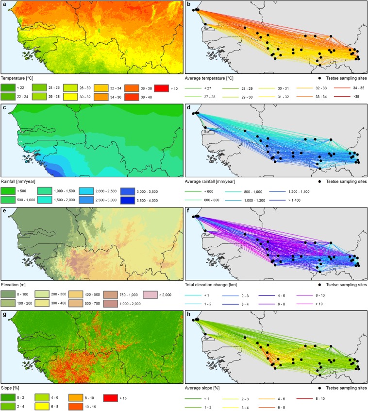
Environmental datasets for genetics. (A) Mean daytime land surface temperature (January 2001–December 2005). (B) Averaged mean daytime land surface temperature along straight lines connecting the entomological sampling sites. (C) Mean rainfall (summed monthly synoptic means for 1960–2000). Source: Worldclim (38). (D) Average rainfall along straight lines connecting the entomological sampling sites. (E) Digital elevation model (57). (F) Total elevation change (both up and down) between entomological sampling sites. (G) Slope. (H) Average slope between entomological sampling sites (both up and down).

Linear Regression Model of the Genetic Distance.

The goal was to find the best environmental predictors of the genetic distance between pairs of tsetse fly populations. We used a linear regression model fitted with generalized least squares (GLS) (29), having the genetic distance (CSE) as the response, and the selected environmental variables as the predictors. The time elapsed between population sampling was forced into the models to control for possible genetic drift. To account for possible autocorrelation, we clustered tsetse populations according to the geographic distance. Hierarchical ascending clustering (Ward method) was used to form partitions of various sizes (from 1 to 19 clusters) based on the Euclidian distance between pairs of populations. Cluster membership was then used to define the grouping structure in the GLS model (30). We selected the eight-cluster partition for which AICc was the lowest with the full GLS model (with all fixed effects) (31). Preliminary analyses revealed that model residuals increased with the fitted genetic distance. To account for this heteroscedasticity, we modeled residuals variance with a power function of the fitted values. Model goodness of fit was assessed using various indicators, including the proportion of variance explained by the fixed effects, quantile–quantile plots of residuals, and the detection of influential observations for GLS coefficients.

Finally, we selected the AICc-best model among all possible submodels in which were forced the Euclidian distance between tsetse populations and the time elapsed between population sampling. Regarding model validation, model selection with Akaike information criteria is formally equivalent to model cross-validation (32). We checked our results with the asymptotically equivalent leave-one-cluster-out cross-validation (CLCV). To do so, we fitted the model to the data with all of the cluster-based groups of distances but one, and predicted the genetic distance with this model for the populations belonging to the left-out group. Prediction errors were then summed for this group, and the process was iterated for all groups. The averaged prediction error was then used as the CLCV indicator to compare the 10 AICc-best models. The first four models were very close in terms of AICc and CLCV, and more generally there was a good agreement between AICc and CLCV (Spearman’s rank correlation of 0.65, P = 0.02).

To build the friction maps, the AICc-best model was used to predict the genetic distance at each pixel location for the different predictors, setting at 0 both the time elapsed between population sampling and the geographical distance.

Building the Least-Cost Paths.

The first iteration of the least-cost paths was based on the initial friction map, as built using the direct paths. Least-cost distances between origin and destination points were calculated using the functions available in the raster and gdistance packages for R (33, 34). Then, averages for all environmental variables were recalculated along the least-cost paths, and Euclidian distances were replaced by the least-cost distances. We subsequently refitted the full model and we selected the AICc-best submodel. The latter was then used to predict the friction across the study region. Finally, we recomputed the least-cost distances based on the updated friction map and iterated this process until the AICc of the best model was stabilized (Fig. 3A). Fig. 3C presents the initial friction and its changes for the first seven iterations. Table S2 and Fig. S6 present the coefficients of the AICc-best model used to build the final friction map and to predict the genetic distance between the potentially isolated tsetse populations associated with the eight habitat clusters (Fig. 5). The dataset including all environmental parameters and the genetic distances between pairs of populations is available as Dataset S1.

Tsetse Distribution Model.

The entomological data used for the regional distribution model of G. p. gambiensis originated from recent baseline surveys for tsetse eradication projects in West Africa: 2007–2008 in Senegal (18), 2008–2009 in Ghana, and 2007–2012 in Burkina Faso (35). Unbaited biconical traps were used in all surveys (36). For the present analysis, only presence/absence data were used. Absence data were filtered by the duration of trapping (≥3 d), and absence data within 5 km from a presence data were discarded. Presence and absence data were also filtered to keep only one presence or absence point within a radius of 5 km. From the initial 2,853 presence and 6,088 absence records, 450 and 516 data points, respectively, were finally retained.

Regarding environmental data used to predict habitat suitability, time series of high-spatial-resolution remote sensing data (1 km) were downloaded, cleaned, and summarized to build relevant environmental and climatic covariates. We combined 11 y of MODIS vegetation and thermal products (January 2003–December 2013). Eight-day composite daytime (DLST) and nighttime land surface temperature (NLST) were extracted from MOD11A2/MYD11A2 temperature and emissivity MODIS products. DLST and NLST were used as proxies for both soil and air temperature, which play an important role in shaping tsetse habitat. Low-quality pixels were removed from the raw data using the quality assessment layer and outliers were filtered using a variant of the boxplot algorithm (37). Vegetation indices at 1 km of spatial resolution and with temporal resolution of 16 d (MOD13A2/MYD13A2) were also downloaded and processed using the quality assessment layer. In particular, the NDVI and middle infrared (MIR) reflectance were selected to describe the vegetation and soil condition in the study area. Temperature and precipitation from WorldClim were also used (38).

A MaxEnt model was used to estimate a habitat suitability index for G. p. gambiensis in the study area (39). The logistic output from this method is a suitability index that ranges between 0 (less suitable habitat) and 1 (highly suitable habitat). The threshold for presence was set to allow a 90% sensitivity (40). Details on the parameterization of MaxEnt and the selection of pseudoabsences are available in Details on the MaxEnt Model.

Identification of Isolated Patches.

To identify the connected patches from the MaxEnt output, we used the function ConnCompLabel in the SDMTools package (41). Then, we used a clustering algorithm to detect clusters of pixels based on their geographical proximity. To this end, we used the function dbscan from the eponymous R package (42). We withdrew isolated pixels as well as those belonging to small clusters (fewer than 20 pixels). Then, we computed the minimum distance between the (centroids of) cluster pixels and those from the general population. We discarded clusters located at less than 10 km from the main tsetse belt because they were unlikely to be genetically isolated from it, and these pixels were thereafter considered as part of the main tsetse belt. Then, we grouped together clusters that were geographically close to each other using a hierarchical ascending classification procedure, with the so-called simple (neighbor-joining) algorithm. At the end of this step, nine clusters were left. One of them was discarded because it was cut by the eastern limit of the analysis window. Finally, we computed the predicted least-cost distance between the clusters and the main tsetse belt using the AICc-best model and the friction raster formerly estimated (Fig. 5 and Table S2). In this sample of eight habitat patches, the correlation of geographic and genetic distances was not significant (Spearman’s rank correlation of 0.43, P = 0.30). To test the significance of the isolation of these clusters, a statistical test was built whereby for each cluster the genetic distance to the main tsetse belt was compared with those between 999 pairs of points randomly generated within the main belt, with the same geographical distance between them as between the patch and the general population (minimum P = 0.001). All genetic distances between pairs of points were computed with the procedure previously described, using the AICc-best model and the friction raster formerly estimated. All analyses were conducted using R software (43).

Environmental Variables and Relationship with the Genetic Distance

We present below the exploration of the relationships between a range of environmental datasets and the CSE (24) measured between 37 populations of G. p. gambiensis (Table S3). Datasets were selected within thematic areas known to play a major role in the ecology, distribution, and dispersal of tsetse flies [i.e., climate (temperature and rainfall), land cover/habitat fragmentation, human population, livestock population, topography, and hydrology]. For each thematic area, one or more datasets were used and a number of potential predictors were derived.

Land-Cover-Based Permeability Indices.

First, we explored the relationship between CSE and expert-based permeability scores. Two land-cover datasets were considered: the Global Land Cover for Africa for the year 2000 (55) (GLC2000) and Globcover 2006 (56) (Fig. S1 A and D). For each of them, permeability scores ranging from 0 to 100 were assigned to each land-cover class present in the study area. The scores were defined by the authors on the basis of the known land-cover preferences of G. p. gambiensis (18, 22). The permeability scores for land-cover classes of GLC2000 and Globcover 2006 are presented in Table S1. The corresponding maps of permeability are presented in Fig. S1 B and E.

Subsequently, the average permeability was calculated along all pairwise connecting lines. The procedure was applied separately to the two land-cover maps, and two sets of permeability indices were derived (Fig. S1 C and F). A nonlinear relationship was observed between the genetic distance and the permeability scores. Because it looked difficult to explain such a shape on an ecological basis, these variables were thus discarded from subsequent analyses. Fig. S4F illustrates the relationship between CSE and Globcover 2006.

Geographical Distance.

Great-circle (straight) distances between the sampled tsetse fly populations were computed using the geographical coordinates (longitude and latitude) of each population, in decimal degrees. A strong linear correlation was observed between this distance and CSE, and it was thus kept for the analysis (Fig. 1). For an easier projection of the model results at the pixel scale, the straight distance was thereafter replaced by the number of pixels crossed along a connecting line. This did not change the nature of the relationship (Fig. S4A).

Average Rainfall and Temperature.

The temperature data were acquired by the NASA MODIS Terra satellite from January 2001 to December 2005. The daytime land surface temperature was used (Fig. S4C). Rainfall data used in this study were based on summed monthly synoptic means for 1960–2000, as derived from WorldClim dataset (Fig. S2C) (38). For both datasets, averaged values were calculated along each line connecting pairwise the entomological sampling sites (Fig. S2 B and D).

Mean daytime land surface temperature was negatively correlated with the mean rainfall. Because the former had a better spatial resolution and was collected from 2001 onward, it was kept for the analysis. A strong linear relationship was observed between CSE and mean daytime land surface temperature (Fig. S4C).

Average Slope and Elevation Change.

Topographical parameters were extracted from elevation data generated by the Shuttle Radar Topography Mission (57). The three-arc-second-resolution, public domain dataset was used (Fig. S2E). For each connecting line, two parameters were estimated: total elevation change, both up and down (58), and average slope (Fig. S2 F and H).

The relationship between the average slope and the genetic distance was not linear and this parameter was not kept in the model (Fig. S4E). The relationship between the elevation change and the genetic distance was linear. However, elevation change was very much correlated to the straight distance. Therefore, we only kept the latter for subsequent analysis.

Human Population Density.

Three sources of human population density were explored: the Gridded Population of the World (59) (GPW) version 3, the Global Rural-Urban Mapping Project (60) (GRUMP), version 1 alpha, and Landscan (61) (Fig. S3). For GPW and GRUMP, the datasets for the reference year 2000 (adjusted to match United Nations totals) were used; for Landscan, an average based on the 10 yearly datasets from 2000 to 2009 was used. For each dataset, the average human population density was calculated along all pairwise connecting lines (Fig. S3 B, D, and F). The best relationship (log-linear) between human population density and genetic distance was observed with the GRUMP data layer (Fig. S4D) and this was thus retained for the model.

Cattle Population Density.

The map of cattle population density was provided by the Gridded Livestock of the World (62). The modeled distribution adjusted to match the FAOSTAT national census totals for the year 2000 was used (Fig. S3G). The average cattle population density was calculated along all pairwise connecting lines (Fig. S3H). There was no strong relationship between genetic distance and cattle density, probably because cattle act in two different ways: On the one hand they are good hosts for G. p. gambiensis, and they can therefore favor passive transport of the flies during herd movements; on the other hand, overgrazing is one of the major causes of landscape degradation, thus reducing active dispersal of the flies. This parameter was thus excluded from the subsequent analysis.

Indices of Habitat Fragmentation.

Indices of habitat fragmentation were based on the percent tree cover (44) for the year 2000 as provided by the MODIS Vegetation Continuous Fields collection 4, version 3. Areas where percentage tree cover was ≥20 were defined as suitable for tsetse (habitat), whereas areas where tree cover was <20 were defined as unsuitable [matrix, following Hanski’s terminology (21)]. The 20% threshold was chosen, somewhat arbitrarily, to maximize the heterogeneity of the fragmentation values calculated between the sampled populations.

All entomological sampling sites were connected pairwise by straight lines, and three linear indices of habitat fragmentation were calculated as mean values along the connecting lines:

• Class area = number of pixels (500 × 500 m) of suitable habitat in the 0.2°-resolution grid over which friction is predicted (Fig. 1, Upper Right);

• Patch density = number of patches of suitable habitat within the 0.2°-resolution pixels (Fig. 1, Lower Left);

• Maximal distance of unsuitable area = Maximum distance between patches within the 0.2°-resolution pixels (Fig. 1, Upper Middle).

Whereas the first two fragmentation indexes characterize landscape composition, the third characterizes landscape shape. We found a negative correlation between the genetic distance and the class area (Fig. 1, Upper Right), which was expected because a higher proportion of suitable habitat should favor dispersal. The relationship between patch density and the genetic distance was not linear (Fig. 1, Lower Left). This was considered as related to the nonlinear relationship between the class area and the patch density (Fig. S5), which is a classical observation in fragmentation processes: When the habitat is not disturbed, the class area is high and the patch density is low (at its most extreme, one single patch occupies the entire pixel). As fragmentation progresses, the class area decreases and the patch density increases. When the class area decreases further, the suitable habitat becomes scarce and the patch density diminishes until it reaches 0 when there is no suitable habitat anymore.

To account for this fragmentation process in the genetic distance model, the patch density was discretized into three categories: “low” when it was <10 patches per pixel, “medium” when it was between 10 and 20 patches per pixel and “high” when it was >20 patches per pixel. It was then used together with its interaction with the class area.

Finally, there was a strong linear relationship between the genetic distance and the maximum distance between patches on a log scale (Fig. 1, Upper Middle). This item was therefore kept in the subsequent analysis. Some of the fragmentation parameters were correlated, such as the class area and the maximum distance of unsuitable area, but they were still kept in the analysis because we formerly reported that for a given class-area value differences in landscape shape can affect habitat suitability for G. p. gambiensis (22).

Hydrological Basin.

For each pair of tsetse sampling sites, it was determined whether they belonged to the same hydrological basin or not (inBasin and outBasin). To this purpose, the HydroSHEDS dataset was used (45) (Fig. 2D).

As expected from the literature and from our knowledge of the ecology of G. p. gambiensis, the presence of a watershed between two sampled populations significantly increased their genetic distances. This variable was thus kept in the model (Fig. 1, Lower Middle). More specifically, riverine tsetse flies such as G. p. gambiensis are known to live very close to water courses. They only move beyond riverine vegetation for feeding (<2 km), and mainly during the rainy season.

Time Difference Between Sampling Events.

Finally, we explored the impact of time difference between sampling events on the genetic distance. Genetic distance is supposed to increase with time (16), as a result of genetic drift. Although the exploratory step did not provide a strong evidence of such an effect (Fig. S4C), we forced this variable in the regression models to control for the possible effect of genetic drift on the observed genetic distances between tsetse populations.

Details on the MaxEnt Model

The methodology used to predict tsetse habitat suitability is based on the framework developed in the Niayes areas (Senegal) (17) and further refined in Burkina Faso in a recent analysis using the MaxEnt model (35). MaxEnt is one of the most widely used species distribution models. It is a machine learning method based on the information theory concept of maximum entropy (39). MaxEnt fits a species distribution by contrasting the environmental conditions where the species is present to the global environment characterized by some generated pseudo-absence data, also called the background. The logistic output gives us a quantitative indicator of the habitat preferences of the species in the study area.

Moreover, to account for the sampling bias present in the entomological data, a Gaussian kernel-based grid that gives more weight to more densely sampled areas was constructed. To build this grid, a smoothing parameter is needed. Five parameters corresponding to the range of maximal dispersal distance of tsetse fly were used (2, 4, 6, 8, and 10 km) (15) to build five bias grids for the MaxEnt models (63, 64). The bias grids were used to sample pseudo-absence from the surveyed area but we also generated and combined pseudo-absence from areas with a high aridity index where there is no suitable habitat for G. p. gambiensis. These areas were selected from the Global Aridity Index dataset (65). Therefore, for each of the five bias grids used, the final pseudo-absence generated is a combination of two generating processes, the first from the bias grid used and the second from the aridity index dataset. In addition to the generation of pseudo-absence, we also accounted for model complexity in the modeling process. In the MaxEnt framework, it can be controlled using the beta regularization parameter. Entomological data were randomly split into two sets, a training set (75% of the total data) and a testing set for further processing. Nine beta regularization parameters (1, 1.5, 2, 2.5, 3, 3.5, 4. 4.5, and 5) were then used to fit a model on the training set, one model for each parameter. Finally, we ended up with nine regularization parameters and five bias grids (one for each smoothing parameter), resulting in 45 models. The final model was an average of the 45 built models. G. p. gambiensis distribution was finally created as a binary map by applying a threshold to the suitability index corresponding to a sensitivity of 90% on the testing set.

References

- 1.WHO . Control and Surveillance of Human African Trypanosomiasis. World Health Organization; Geneva: 2013. [PubMed] [Google Scholar]
- 2.Swallow BM, editor. Impacts of Trypanosomiasis on African Agriculture. FAO; Rome: 2000. [Google Scholar]
- 3.Alsan M. The effect of the tsetse fly on African development. Am Econ Rev. 2015;105(1):382–410. [Google Scholar]
- 4.Bouyer F, et al. Ex-ante benefit-cost analysis of the elimination of a Glossina palpalis gambiensis population in the Niayes of Senegal. PLoS Negl Trop Dis. 2014;8(8):e3112. doi: 10.1371/journal.pntd.0003112. [DOI] [PMC free article] [PubMed] [Google Scholar]
- 5.Vreysen MJB, Seck MT, Sall B, Bouyer J. Tsetse flies: Their biology and control using area-wide integrated pest management approaches. J Invertebr Pathol. 2013;112(Suppl):S15–S25. doi: 10.1016/j.jip.2012.07.026. [DOI] [PubMed] [Google Scholar]
- 6.Kgori PM, Modo S, Torr SJ. The use of aerial spraying to eliminate tsetse from the Okavango Delta of Botswana. Acta Trop. 2006;99(2-3):184–199. doi: 10.1016/j.actatropica.2006.07.007. [DOI] [PubMed] [Google Scholar]
- 7.Vreysen MJB, et al. Glossina austeni (Diptera: Glossinidae) eradicated on the island of Unguja, Zanzibar, using the sterile insect technique. J Econ Entomol. 2000;93(1):123–135. doi: 10.1603/0022-0493-93.1.123. [DOI] [PubMed] [Google Scholar]
- 8.Solano P, et al. The population structure of Glossina palpalis gambiensis from island and continental locations in Coastal Guinea. PLoS Negl Trop Dis. 2009;3(3):e392. doi: 10.1371/journal.pntd.0000392. [DOI] [PMC free article] [PubMed] [Google Scholar]
- 9.Solano P, et al. Population genetics as a tool to select tsetse control strategies: Suppression or eradication of Glossina palpalis gambiensis in the Niayes of Senegal. PLoS Negl Trop Dis. 2010;4(5):e692. doi: 10.1371/journal.pntd.0000692. [DOI] [PMC free article] [PubMed] [Google Scholar]
- 10.Koné N, et al. Contrasting population structures of two vectors of African trypanosomoses in Burkina Faso: Consequences for control. PLoS Negl Trop Dis. 2011;5(6):e1217. doi: 10.1371/journal.pntd.0001217. [DOI] [PMC free article] [PubMed] [Google Scholar]
- 11.Vreysen MJ, et al. Release-recapture studies confirm dispersal of Glossina palpalis gambiensis between river basins in Mali. PLoS Negl Trop Dis. 2013;7(4):e2022. doi: 10.1371/journal.pntd.0002022. [DOI] [PMC free article] [PubMed] [Google Scholar]
- 12.Spear SF, Balkenhol N, Fortin M-J, McRae BH, Scribner K. Use of resistance surfaces for landscape genetic studies: Considerations for parameterization and analysis. Mol Ecol. 2010;19(17):3576–3591. doi: 10.1111/j.1365-294X.2010.04657.x. [DOI] [PubMed] [Google Scholar]
- 13.Zeller KA, McGarigal K, Whiteley AR. Estimating landscape resistance to movement: A review. Landscape Ecol. 2012;27(6):777–797. [Google Scholar]
- 14.Peterman WE, Connette GM, Semlitsch RD, Eggert LS. Ecological resistance surfaces predict fine-scale genetic differentiation in a terrestrial woodland salamander. Mol Ecol. 2014;23(10):2402–2413. doi: 10.1111/mec.12747. [DOI] [PubMed] [Google Scholar]
- 15.Bouyer J, et al. Population sizes and dispersal pattern of tsetse flies: Rolling on the river? Mol Ecol. 2009;18(13):2787–2797. doi: 10.1111/j.1365-294X.2009.04233.x. [DOI] [PubMed] [Google Scholar]
- 16.De Meeûs T, Ravel S, Rayaisse J-B, Courtin F, Solano P. Understanding local population genetics of tsetse: The case of an isolated population of Glossina palpalis gambiensis in Burkina Faso. Infect Genet Evol. 2012;12(6):1229–1234. doi: 10.1016/j.meegid.2012.04.005. [DOI] [PubMed] [Google Scholar]
- 17.Dicko AH, et al. Using species distribution models to optimize vector control in the framework of the tsetse eradication campaign in Senegal. Proc Natl Acad Sci USA. 2014;111(28):10149–10154. doi: 10.1073/pnas.1407773111. [DOI] [PMC free article] [PubMed] [Google Scholar]
- 18.Bouyer J, Seck MT, Sall B, Guerrini L, Vreysen MJB. Stratified entomological sampling in preparation of an area-wide integrated pest management programme: The example of Glossina palpalis gambiensis in the Niayes of Senegal. J Med Entomol. 2010;47(4):543–552. doi: 10.1093/jmedent/47.4.543. [DOI] [PMC free article] [PubMed] [Google Scholar]
- 19.International Glossina Genome Initiative Genome sequence of the tsetse fly (Glossina morsitans): Vector of African trypanosomiasis. Science. 2014;344(6182):380–386. doi: 10.1126/science.1249656. [DOI] [PMC free article] [PubMed] [Google Scholar]
- 20.Hendrichs J, Vreysen MJB, Enkerlin WR, Cayol JP. Strategic options in using sterile insects for area-wide integrated pest management. In: Dyck VA, Hendrichs J, Robinson AS, editors. Sterile Insect Technique. Springer; Dordrecht, The Netherlands: 2005. pp. 563–600. [Google Scholar]
- 21.Hanski I, Ovaskainen O. The metapopulation capacity of a fragmented landscape. Nature. 2000;404(6779):755–758. doi: 10.1038/35008063. [DOI] [PubMed] [Google Scholar]
- 22.Guerrini L, Bord JP, Ducheyne E, Bouyer J. Fragmentation analysis for prediction of suitable habitat for vectors: Example of riverine tsetse flies in Burkina Faso. J Med Entomol. 2008;45(6):1180–1186. doi: 10.1603/0022-2585(2008)45[1180:fafpos]2.0.co;2. [DOI] [PubMed] [Google Scholar]
- 23.Wright S. The interpretation of population structure by F-statistics with special regard to system of mating. Evolution. 1965;19(3):395–420. [Google Scholar]
- 24.Cavalli-Sforza LL, Edwards AWF. Phylogenetic analysis. Models and estimation procedures. Am J Hum Genet. 1967;19(3 Pt 1):233–257. [PMC free article] [PubMed] [Google Scholar]
- 25.Bowcock AM, et al. High resolution of human evolutionary trees with polymorphic microsatellites. Nature. 1994;368(6470):455–457. doi: 10.1038/368455a0. [DOI] [PubMed] [Google Scholar]
- 26.de Meeûs T, et al. Population genetics and molecular epidemiology or how to “débusquer la bête”. Infect Genet Evol. 2007;7(2):308–332. doi: 10.1016/j.meegid.2006.07.003. [DOI] [PubMed] [Google Scholar]
- 27.Takezaki N, Nei M. Genetic distances and reconstruction of phylogenetic trees from microsatellite DNA. Genetics. 1996;144(1):389–399. doi: 10.1093/genetics/144.1.389. [DOI] [PMC free article] [PubMed] [Google Scholar]
- 28.Kalinowski ST. Evolutionary and statistical properties of three genetic distances. Mol Ecol. 2002;11(8):1263–1273. doi: 10.1046/j.1365-294x.2002.01520.x. [DOI] [PubMed] [Google Scholar]
- 29.Laird NM, Ware JH. Random-effects models for longitudinal data. Biometrics. 1982;38(4):963–974. [PubMed] [Google Scholar]
- 30.Dormann CF, et al. Methods to account for spatial autocorrelation in the analysis of species distributional data: A review. Ecography. 2007;30(5):609–628. [Google Scholar]
- 31.Hurvich CM, Tsai C-L. Model selection for extended quasi-likelihood models in small samples. Biometrics. 1995;51(3):1077–1084. [PubMed] [Google Scholar]
- 32.Fang Y. Asymptotic equivalence between cross-validations and Akaike Information Criteria in mixed-effects models. J Data Sci. 2011;9:15–21. [Google Scholar]
- 33.Hijmans RJ. 2015. raster: Geographic data analysis and modeling, R package version 2.4-15. Available at https://cran.r-project.org/web/packages/raster/index.html.
- 34.van Etten J. 2012 gdistance: Distances and routes on geographical grids, R package version 1:1-4. Available at CRAN.R-project.org/package=gdistance.
- 35.Dicko AH, et al. A spatio-temporal model of African animal trypanosomosis risk. PLoS Negl Trop Dis. 2015;9(7):e0003921. doi: 10.1371/journal.pntd.0003921. [DOI] [PMC free article] [PubMed] [Google Scholar]
- 36.Challier A, Laveissière C. Un nouveau piège pour la capture des glossines (Glossina: Diptera, Muscidae): Description et essais sur le terrain. Cah ORSTOM sér Ent Méd Parasitol. 1973;10(4):251–262. [Google Scholar]
- 37.Neteler M. Estimating daily land surface temperatures in mountainous environments by reconstructed MODIS LST data. Remote Sens. 2010;2(1):333–351. [Google Scholar]
- 38.Hijmans R, Cameron S, Parra J, Jones P, Jarvis A. Very high resolution interpolated climate surfaces for global land areas. Int J Climatol. 2005;25:1965–1978. [Google Scholar]
- 39.Elith J, et al. A statistical explanation of MaxEnt for ecologists. Divers Distrib. 2011;17(1):43–57. [Google Scholar]
- 40.Liu C, Berry PM, Dawson TP, Pearson RG. Selecting thresholds of occurrence in the prediction of species distributions. Ecography. 2005;28(3):385–393. [Google Scholar]
- 41.VanDerWal J, Falconi L, Januchowski S, Shoo L, Storlie C. 2014 SDMTools: Species distribution modelling tools: Tools for processing data associated with species distribution modelling exercises, R package version 1.1-221. Available at https://cran.r-project.org/web/packages/SDMTools/index.html.
- 42.Hahsler M. 2015. dbscan: Density Based Clustering of Applications with Noise (DBSCAN), R package version 0.9-1. Available at https://cran.r-project.org/web/packages/dbscan/index.html.
- 43.R Core Team 2015 R: A language and environment for statistical computing (R Foundation for Statistical Computing, Vienna). Available at www.R-project.org.
- 44.Hansen M, et al. Global percent tree cover at a spatial resolution of 500 meters: First results of the MODIS vegetation continuous fields algorithm. Earth Interact. 2003;7(10):1–15. [Google Scholar]
- 45.Lehner B, Verdin K, Jarvis A. New global hydrography derived from spaceborne elevation data. Eos. 2008;89(10):93–94. [Google Scholar]
- 46.Solano P, Duvallet G, Dumas V, Cuisance D, Cuny G. Microsatellite markers for genetic population studies in Glossina palpalis (Diptera: Glossinidae) Acta Trop. 1997;65(3):175–180. doi: 10.1016/s0001-706x(97)00663-3. [DOI] [PubMed] [Google Scholar]
- 47.Luna C, et al. Microsatellite polymorphism in tsetse flies (Diptera: Glossinidae) J Med Entomol. 2001;38(3):376–381. doi: 10.1603/0022-2585-38.3.376. [DOI] [PubMed] [Google Scholar]
- 48.Baker MD, Krafsur ES. Identification and properties of microsatellite markers in tsetse flies Glossina morsitans sensu lato (Diptera: Glossinidae) Mol Ecol Notes. 2001;1(4):234–236. doi: 10.1046/j.1471-8278.2001.00087.x. [DOI] [PMC free article] [PubMed] [Google Scholar]
- 49.De Meeûs T, Guégan JF, Teriokhin AT. MultiTest V.1.2, a program to binomially combine independent tests and performance comparison with other related methods on proportional data. BMC Bioinformatics. 2009;10:443. doi: 10.1186/1471-2105-10-443. [DOI] [PMC free article] [PubMed] [Google Scholar]
- 50.Goudet J. FSTAT (v. 1.2): A computer program to calculate F-statistics. J Hered. 1995;86(6):485–486. [Google Scholar]
- 51.Van Oosterhout C, Hutchinson WF, Wills DPM, Shipley P. MICRO-CHECKER: Software for identifying and correcting genotyping errors in microsatellite data. Mol Ecol Notes. 2004;4(3):535–538. [Google Scholar]
- 52.Brookfield JFY. A simple new method for estimating null allele frequency from heterozygote deficiency. Mol Ecol. 1996;5(3):453–455. doi: 10.1111/j.1365-294x.1996.tb00336.x. [DOI] [PubMed] [Google Scholar]
- 53.Dieringer D, Schlötterer C. Microsatellite analyser (MSA): A platform independent analysis tool for large microsatellite data sets. Mol Ecol Notes. 2003;3(1):167–169. [Google Scholar]
- 54.Coombs JA, Letcher BH, Nislow KH. create: A software to create input files from diploid genotypic data for 52 genetic software programs. Mol Ecol Resour. 2008;8(3):578–580. doi: 10.1111/j.1471-8286.2007.02036.x. [DOI] [PubMed] [Google Scholar]
- 55.Mayaux P, Bartholomé E, Fritz S, Belward A. A new land-cover map of Africa for the year 2000. J Biogeogr. 2004;31(6):861–877. [Google Scholar]
- 56.Arino O, et al. IEEE International Geoscience and Remote Sensing Symposium, 2007. IEEE; New York: 2007. GlobCover: ESA service for global land cover from MERIS; pp. 2412–2415. [Google Scholar]
- 57.Van Zyl JJ. The Shuttle Radar Topography Mission (SRTM): A breakthrough in remote sensing of topography. Acta Astronaut. 2001;48(5):559–565. [Google Scholar]
- 58.Keyghobadi N, Roland J, Strobeck C. Influence of landscape on the population genetic structure of the alpine butterfly parnassius smintheus (Papilionidae) Mol Ecol. 1999;8(9):1481–1495. doi: 10.1046/j.1365-294x.1999.00726.x. [DOI] [PubMed] [Google Scholar]
- 59.Balk D, Yetman G. The Global Distribution of Population: Evaluating the Gains in Resolution Refinement. Center for International Earth Science Information Network, Columbia Univ; New York: 2004. [Google Scholar]
- 60.Center for International Earth Science Information Network, Columbia University International Food Policy Research Institute, the World Bank, and Centro Internacional de Agricultura Tropical . Global Rural-Urban Mapping Project (GRUMP): Urban/Rural Population Grids. Center for International Earth Science Information Network, Columbia Univ; Palisades, NY: 2004. [Google Scholar]
- 61.Dobson J, Bright E, Coleman P, Durfee R, Worley B. LandScan: A global population database for estimating populations at risk. Photogramm Eng Remote Sensing. 2000;66(7):849–857. [Google Scholar]
- 62.Wint W, Robinson TP. Gridded Livestock of the World 2007. FAO; Rome: 2007. [PubMed] [Google Scholar]
- 63.Dudík M, Phillips SJ, Schapire RE. Advances in Neural Information Processing Systems. MIT Press; Cambridge, MA: 2005. Correcting sample selection bias in maximum entropy density estimation; pp. 323–330. [Google Scholar]
- 64.Phillips SJ, et al. Sample selection bias and presence-only distribution models: Implications for background and pseudo-absence data. Ecol Appl. 2009;19(1):181–197. doi: 10.1890/07-2153.1. [DOI] [PubMed] [Google Scholar]
- 65.Zomer RJ, Trabucco A, Bossio DA, Verchot LV. Climate change mitigation: A spatial analysis of global land suitability for clean development mechanism afforestation and reforestation. Agric Ecosyst Environ. 2008;126(1):67–80. [Google Scholar]
Associated Data
This section collects any data citations, data availability statements, or supplementary materials included in this article.