Measuring Electric Fields and Noncovalent Interactions Using the Vibrational Stark Effect

CONSPECTUS

Over the past decade, we have developed a spectroscopic approach to measure electric fields inside matter with high spatial (<1 Å) and field (<1 MV/cm) resolution. The approach hinges on exploiting a physical phenomenon known as the vibrational Stark effect (VSE), which ultimately provides a direct mapping between observed vibrational frequencies and electric fields. Therefore, the frequency of a vibrational probe encodes information about the local electric field in the vicinity around the probe. The VSE method has enabled us to understand in great detail the underlying physical nature of several important biomolecular phenomena, such as drug–receptor selectivity in tyrosine kinases, catalysis by the enzyme ketosteroid isomerase, and unidirectional electron transfer in the photosynthetic reaction center. Beyond these specific examples, the VSE has provided a conceptual foundation for how to model intermolecular (noncovalent) interactions in a quantitative, consistent, and general manner.

The starting point for research in this area is to choose (or design) a vibrational probe to interrogate the particular system of interest. Vibrational probes are sometimes intrinsic to the system in question, but we have also devised ways to build them into the system (extrinsic probes), often with minimal perturbation. With modern instruments, vibrational frequencies can increasingly be recorded with very high spatial, temporal, and frequency resolution, affording electric field maps correspondingly resolved in space, time, and field magnitude.

In this Account, we set out to explain the VSE in broad strokes to make its relevance accessible to chemists of all specialties. Our intention is not to provide an encyclopedic review of published work but rather to motivate the underlying framework of the methodology and to describe how we make and interpret the measurements. Using certain vibrational probes, benchmarked against computer models, it is possible to use the VSE to measure absolute electric fields in arbitrary environments. The VSE approach provides an organizing framework for thinking generally about intermolecular interactions in a quantitative way and may serve as a useful conceptual tool for molecular design.

Graphical abstract

1. MOTIVATION AND BACKGROUND

Much of contemporary chemistry is concerned with non-covalent interactions, as predicted by J.-M. Lehn nearly a quarter-century ago.¹ Noncovalent interactions form the basis of molecular recognition, enabling matter to self-organize and emerge into complex structures. For these reasons, it is the recurring leitmotif of molecular biology² (nucleic acid base-pairing, receptor–ligand specificity, protein folding, enzyme catalysis, membrane biophysics) and is increasingly exploited in new frontiers of synthesis based on self-assembly (DNA origami, crystal engineering,³ reticular/framework materials,⁴ and hybrid materials).

Despite the importance and ubiquity of noncovalent (intermolecular) interactions, it has been challenging for chemists to identify the right language to describe them. The dissociation constant (K_D) is certainly a common descriptor, but what it possesses in generality, it lacks in molecular insight. Dissociation constants do not identify what portions of the molecules are responsible for an interaction. Moreover, they depend on macroscopic parameters (temperature and pressure) and are difficult to relate to (or even calculate from⁵) the microscopic arrangement of molecules in a given system. These limitations pose challenges for the chemist interested in predicting properties of noncovalent interactions, issues at the heart of numerous synthetic challenges such as drug design. Conventionally, chemists address this problem by extending the concept of the covalent bond to describe noncovalent interactions, for example, hydrogen bonds (H-bonds), halogen bonds (X-bonds), π-stacking, cation–π bonds, charge-transfer interactions.⁶ However, these terms for specific interactions are often based on arbitrary geometric criteria (indeed, there is still debate as to what “counts” as a H-bond⁷), and their ability to explain or predict energetics is limited to ranges or ballpark values.

In our view, the usage of bonding concepts to describe intermolecular interactions is problematic because it belies the fact that most of these interactions are electrostatic (can be explained well without orbitals or electron densities) and because it ignores the nonspecific interactions (e.g., dipole–dipole, dipole-induced dipole) that can be just as energetically significant as the specific interactions attached special labels.⁶ What is needed is a model for intermolecular interactions that does not depend on assigning labels or cutoffs, applies equally to specific and nonspecific interactions, and is quantitative and microscopic. We believe the electric field, a fundamental concept from physics, is a conceptual tool that meets all these criteria.

Figure 1A illustrates the simple principles governing the interaction between a dipole and an external field: if the dipole is not aligned with the field, it is in a configuration of high energy; the field exerts a torque and rotates the dipole to align with it to give the lowest energy configuration. The energy depends on the dipole magnitude, the field magnitude, and their relative orientation as $U=-\overrightarrow{\mu }\cdot \overrightarrow{F}$ where $\overrightarrow{F}$denotes electric field and $\overrightarrow{\mu }$ denotes dipole moment. Now consider a solute molecule (represented as a green circle) solvated by an aqueous environment (Figure 1B). In a chemical picture that consists of atoms and orbitals, a quantum mechanical calculation is needed to determine the interaction energy between solute and environment. However, many simple molecules can be represented as a point dipole (and complex molecules as a collection of dipoles) and the other molecules in the environment can be viewed as creating an electric field (represented with red field lines, Figure 1C) through their own charges, dipoles, induced dipoles, etc. In this picture, the interaction between a molecule and its surrounding environment can be recast as an interaction between a dipole and an electric field. This picture is quantitative and holds as long as there is no (or little) covalent character to the interaction.

Figure 1.

Connection between electric fields and molecular interactions. (A) When a voltage is applied between two parallel plates, charge accumulates on the surfaces to create a uniform electric field, $\overrightarrow{F}$. Dipole moments interact with electric fields according to the equation $U=-\overrightarrow{\mu }\cdot \overrightarrow{F}$. (B) Determining the interaction energy between molecules is generally a quantum mechanical problem. However, if we focus on one molecule and consider it as a dipole interacting with the field created by all the other molecules, the chemical picture can be converted into an electrostatic one (C).

By electric field, we mean specifically the electric field due to the environment, that is, not that due to the atoms that are part of the same molecule as the one that is said to experience the field. Interactions between atoms in the same molecule must be treated quantum mechanically. In this definition, atoms on an isolated molecule (as in the gas phase) experience zero electric field. Although arbitrary on some level, this definition amounts to choosing a useful reference state since our primary goal is to use electrostatic concepts to describe intermolecular interactions.

The picture in Figure 1C gives us a quantity (the electric field) that we can attach to a given environment (a protein, a solvent, a host) and tells us the energetic value associated with inserting a molecule (a ligand, a solute, a guest) into that environment at a particular position and orientation. More than just being an abstract concept though, the electric field can be measured using the vibrational Stark effect (VSE, section 2), enabling comparisons between very different systems (section 3), and can be easily computed with molecular mechanics models (section 2.3).

2. THE VIBRATIONAL STARK EFFECT

2.1. Vibrational Stark Spectroscopy (VSS)

Consider the molecular potential energy curve for a diatom such as CO (Figure 2A). These potentials are anharmonic, and one consequence of this is that when a molecule goes to higher vibrational energy levels, its bond lengthens slightly ( $\mathrm{\Delta }\overrightarrow{d}$). Note that the magnitude of $\overrightarrow{d}$, $\left|\overrightarrow{d}\right|$ or simply d, denotes the CO bond length, and its direction, $\widehat{d}$, denotes the orientation of the CO bond axis. If this diatom possess a charge separation (q), that is, it possesses a permanent dipole moment, then its dipole moment will be slightly larger in the first vibrational excited state compared with the ground state: ${\overrightarrow{\mu }}_0=q\overrightarrow{d},{\overrightarrow{\mu }}_1=q(\overrightarrow{d}+\mathrm{\Delta }\overrightarrow{d})$. Infrared (IR) and Raman spectroscopies probe the energy gap between the ground and first excited vibrational state. Since these states have (slightly) different dipoles, they will be (de)stabilized (slightly) differently by an external field, ${\overrightarrow{F}}_{\mathrm{ext}}$ (Figure 2B), depending on the orientation between the dipole and the field. Therefore, the applied electric field will produce a shift in the vibrational transition energy that is linear with the difference in the dipole moments of the two vibrational states, $\mathrm{\Delta }\overrightarrow{\mu }:\mathrm{\Delta }\overrightarrow{v}=-\mathrm{\Delta }\overrightarrow{\mu }\cdot {\overrightarrow{F}}_{\mathrm{ext}}$. A vibration’s difference dipole is directly related to the vibrational frequency’s sensitivity to an external electric field, and so it is referred to as the Stark tuning rate. Vibrational Stark tuning rates are measured to be around 0.5–2cm⁻¹/(MV/cm). The unit corresponds to the frequency shift (in cm⁻¹) that would accompany the application of a unit electric field (1 MV/cm) projected along the vibrational axis. These tuning rates imply vibrational difference dipoles of 0.03–0.12 D (i.e., 1 D = 16.8 cm⁻¹/(MV/cm)). A polyatomic molecule has a more complex electrostatic and vibrational structure. However, if we limit our attention to high-frequency vibrations of specific functional groups (such as C=O or C≡N stretches), we find that they are largely decoupled from the rest of the molecule and behave similarly to the diatom (called one-dimensional behavior).⁸ This implies that $\mathrm{\Delta }\overrightarrow{\mu }$ for such a vibrational transition is colinear with the vibrational mode’s bond axis.

Figure 2.

Vibrational Stark effect can be explained in terms of anharmonicity. (A) The anharmonic form of molecular potential energy surfaces implies that bonds will be slightly longer (and so possess slightly larger dipole moments) in their vibrational excited states; $\widehat{d}$ denotes the unit vector aligned with the CO bond axis. (B) Therefore, ground and excited vibrational states are stabilized differently by an electric field, resulting in a shift in the transition energy (vibrational frequency).

Because the difference dipole arises from mechanical anharmonicity, it can be calculated from experimental quantities by finding q (for a diatom, simply ${\overrightarrow{\mu }}_0/\overrightarrow{d}$) and multiplying by $\left|\mathrm{\Delta }\overrightarrow{d}\right|$ (related to the difference in the gas-phase 1 ← 0 and 2 ← 1 transition energies). Values obtained from this kind of simple calculation are shown in Table S1 in the Supporting Information. Difference dipoles can also be calculated with ab initio methods. Experimentally, the difference dipole can be measured in two different ways. The most straightforward method consists of accurately measuring the molecule’s dipole moment in the ground and vibrationally excited states and taking the difference; the accuracy required limits the scope of this approach to a few small gaseous molecules. A more general approach is vibrational Stark spectroscopy (VSS), in which external fields are applied to molecules and the effect on the vibrational spectrum is recorded (see Table S1, Supporting Information for examples and comparisons).⁹

In VSS (Figure 3A), a molecule containing the vibration of interest is first immobilized by embedding it in a polymer film or dissolving it in a glass-forming solvent that is rapidly cooled by immersion into liquid nitrogen. The glassy matrix fills a transparent capacitor, in which parallel plates are displaced ca. 20 μm. Voltages on the order of 1–2 kV are achievable before dielectric breakdown, resulting in applied electric fields as large as ∼1 MV/cm.⁹ The measurement consists of acquiring the IR spectrum of the sample in the presence and absence of the applied electric field. By analyzing the small differences between the spectra, the vibration’s difference dipole can be determined.^9,10 For most vibrations that we have studied, the frequency responds to the external field in a linear fashion. In the difference spectrum, this effect manifests as a second derivative line shape (the interested reader should consult refs 9 and 10 for details on this analysis).

Figure 3.

Calibrating frequency shifts to changes in electric field. (A) In vibrational Stark spectroscopy, external electric fields are applied to a frozen isotropic sample, and the perturbation caused to the infrared spectrum is recorded. For many molecules, the response is linear and the experiment yields the linear Stark tuning rate. (B) Frequency shifts (as measured by FT-IR spectroscopy) caused by changing the environment surrounding a molecule can be translated into electric field differences projected along the CO bond, using the Stark tuning rate as the conversion factor. Adapted with permission from refs 19 and 20. Copyright 1999 and 1994 American Chemical Society.

Stark tuning rates have now been determined for many vibrations: O–H,¹¹ N–H and S–H,¹² C=O,^13,14 C≡N,^15–17 azide,¹⁷ and C–D. In VSS, all of these vibrations respond to an external field in a mostly linear fashion. There is however one major limitation to VSS that complicates the experiment’s interpretation, and that is the local field effect:^9,18 What we measure is not $\left|\mathrm{\Delta }\overrightarrow{\mu }\right|$, but $\left|\mathrm{\Delta }\overrightarrow{\mu }\right|f$, where f (the local field correction factor) is a scalar whose value we estimate to be ∼2. How we arrived at this estimate and its importance requires a lengthier and more technical discussion and is provided as a Supporting Information to this Account.

2.2. Vibrational Stark Effects to Probe Electric Fields

The VSE method treats the difference dipole as a sensitivity parameter that enables subsequently measured IR frequency shifts to be interpreted in terms of changes in electric field (Figure 3B). For example, if a vibration on a ligand (e.g., the C≡O stretch of heme–CO) has a Stark tuning rate $\left|\mathrm{\Delta }\overrightarrow{\mu }\right| ={1\mathrm{cm}}^{-1}/\left(\mathrm{MV}/\mathrm{cm}\right)$ and its vibrational frequency shifts by 28 cm⁻¹ to the red when the vibrational probe is surrounded by a protein environment relative to a nonpolar solvent, then we would assert it experiences an electric field (projected along the CO bond axis) more stabilizing by 28 MV/cm in the binding site $(\mathrm{\Delta }{\overrightarrow{F}}_{\mathrm{solvent}\to \text{binding site}}\cdot {\widehat{d}}_{\mathrm{CO}}=\mathrm{\Delta }{\overline{v}}_{\mathrm{CO}}/|\mathrm{\Delta }{\overrightarrow{\mu }}_{\mathrm{CO}}|)$.¹⁹ This information could provide a physical basis for (some of) the driving force for the ligand to bind to the protein. Similarly, frequency shifts accompanying a mutation (which can also be similarly large) can be interpreted in terms of changes in protein electric field due to the mutation (Figure 3B).²⁰ To interpret these frequency shifts in proteins, structural data is needed to determine the orientation of the vibrational probe ( ${\widehat{d}}_{\mathrm{CO}}$) with respect to the protein field.

These assertions make two assumptions: first, that the frequency’s linear dependence on field, which is only shown from VSS for field perturbations of order 1 MV/cm, is also the case for the larger perturbation caused by the binding pocket; second, that the vibrational frequency shift due to changes in the environment can be fully attributed to an electric field effect. In the next section, we show how computational methods helped us test these critical assumptions. Chemists are accustomed to interpreting vibrational frequency shifts as changes in bonds’ force constants (i.e., $\overline{v}={\left(2\pi \right)}^{-1}{(k/m)}^{1/2}$), arising from changes in either bond order or bond strength. In applying the VSE to interpret frequency shifts associated with intermolecular interactions, we assume that the force constants (and intramolecular properties in general) are constant as the environment changes; for instance, the VSE would not explain the frequency shift between free CO and heme–CO. In practice, this assumption can be experimentally tested because a frequency shift due to a change in force constant would also result in a change in the difference dipole (measured by VSS) and anharmonicity (measured by overtone spectroscopy or 2-D IR). We find for many vibrations that frequencies can shift substantially among different environments without a noticeable change in the difference dipole, ruling out the changing force constant model; some vibrations involving hydrogen (S–H and N–H) are a notable exception.¹²

2.3. Solvatochromic Calibration

In VSS, when we take the IR spectrum of a solute in the glassy matrix, the peak frequency is very different from that molecule’s peak frequency in the gas phase, even before the external electric field is turned on. To a large extent, this shift is also a Stark effect, except it arises from the field created by the matrix^18,21 (i.e., the surrounding molecules’ dipoles as illustrated by Figure 1C) instead of by an external voltage. Building on this concept, we can imagine a much easier experiment than VSS, wherein we vary the field on a vibrational probe not with a voltage source but by dissolving it in solvents of various polarities.^22,23 Liquid solvents will exert an electric field (termed the solvent reaction field) in proportion to how polar the solvent is (a more polar solvent molecule will possess larger dipoles)^24,25 and how polar the solute is (a more polar solute will force the solvent to organize less randomly around it).^25,26 However, solvent electric fields cannot be precisely controlled by an experimentalist, and so ascribing them specific values requires a model.

Dielectric constants and empirical polarity scales are useful ways to characterize solvents, but they are difficult to relate to the system’s microscopic structure. We have demonstrated that solvent-induced vibrational frequency shifts are effectively Stark effects. In one test of this, we found that a vibrational probe’s sensitivity to solvent variation (i.e., the frequency shift across a given range of solvents) is directly proportional to the probe’s difference dipole (Figure 4A,B). For instance, acetophenone’s C=O vibration has approximately twice the Stark tuning rate of benzonitrile’s C≡N (Figure 4A shows two schematic Stark spectra). We would then predict that acetophenone’s band would shift twice as much as benzonitrile’s in response to solvatochromic effects, which indeed turns out to be the case (shown schematically in Figure 4B), so $\mathrm{\Delta }{\overline{v}}_{\mathrm{solv}}$ is proportional to $\left|\mathrm{\Delta }\overrightarrow{\mu }\right|$. This relationship was also obtained for (1) two isotopologues of phenol, Ph–OH and Ph-OD,¹¹ (2) a set of aminobenzonitrile positional isomers,²⁷ and (3) a set of carbonyls with various degrees of conjugation (unpublished results). The proportionality is more quantitative when considering similar solutes. This test is important because it is independent of the values of the solvent fields.

Figure 4.

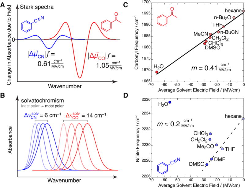
Connection between solvent-induced vibrational frequency shifts (solvatochromism) and the Stark effect. (A) Idealized Stark spectra of benzonitrile¹⁹ and acetophenone.¹⁸ Stark spectra for vibrations typically have a second-derivative line shape whose amplitude scales as the square of $\left|\mathrm{\Delta }\overrightarrow{\mu }\right|f$. (B) Idealized absorption spectra of benzonitrile³² and acetophenone¹⁸ in solvents of increasing polarity. The span in frequency shift over a given range of solvent polarity is proportional to the Stark tuning rate. More polar solvents give more red-shifted (and broader) bands. (C) The solvent-dependent frequency of the C=O vibration of acetophenone is explained by the calculated solvent electric field and the C=O vibration’s difference dipole. The slope, m, is a measure of $\left|\mathrm{\Delta }\overrightarrow{\mu }\right|$, and is 2.5-fold smaller than $\left|\mathrm{\Delta }\overrightarrow{\mu }\right|f$, obtained from the vibrational Stark spectrum. This is consistent with our current view that the local field correction factor, f ≈ 2 (see the Supporting Information). (D) The solvent-dependent frequency of the CN vibration of benzonitrile is not well explained by the solvent electric field, implying the necessity for a more complex model to describe its frequency (see main text). Adapted with permission from refs 14, 15, and 29. Copyright 2013, 2000, and 2012 American Chemical Society.

A second test that is more stringent but also more model-dependent involves correlating the solvent-by-solvent frequency variation for an individual solute against the average solvent field calculated for each solvent, as shown in Figure 4C,D.^28,29 The strategy we have generally adopted for these calculations is molecular dynamics (MD) simulations, though Poisson–Boltzmann and the Onsager models can give similar results with some caveats.²⁸ For some solutes, these curves are linear over the full range of electric fields spanned by solvent variation and include solvents that can participate in specific interactions (H-bonds and X-bonds) with the vibrational probe. This behavior has been observed for several molecules’ C=O vibrations (acetophenone’s is shown in Figure 4C) and O–H vibrations. Solvent fields (order tens of MV/cm) can be large relative to the largest achievable external fields in a capacitor (order 1 MV/cm) because of the short distances on which molecular interactions act.

The solvent field-frequency relationships affirm the two earlier assumptions about the VSE: that its linearity can extend over a wider domain than that directly observed in VSS and that it is sufficient to explain almost all variation in frequency across solvents with very different chemical compositions and H-bonding capacities.¹⁴ The field-frequency curve additionally allows us to map the observed frequency in an arbitrary environment to the average absolute electric field.

The extra word “average” is important because solvent molecules’ positions fluctuate, so the instantaneous solvent electric field for a given configuration can be very different from the mean of the field distribution sampled by the solvation dynamics. The peak position of a vibrational probe only conveys information about the ensemble-average electric field; on the other hand, the line width of a vibrational probe’s band is related to the dispersion in electric fields associated with an environment (i.e., its inhomogeneity).

A significant datum in Figure 4C is the point for water, which produces a considerably larger bathochromic shift than other solvents, and is also calculated to exert proportionally larger electric fields. This finding is suggestive that the H-bonding interaction is amenable to an electrostatic description, and that we can think of its greater strength relative to a dipole–dipole interaction in terms of its capacity to generate a greater electric field. This feature is central to our picture that electric fields serve as a unifying concept to compare specific and nonspecific interactions on an equal footing.

We arrived at this conclusion using the carbonyl vibration’s simple frequency variation (that is, a “pure” linear Stark effect). This property is not universal. For instance, a great deal of work on the VSE has focused on the nitrile probe because of its appearance in an uncluttered window in the mid-IR (ca. 2200 cm⁻¹), the many methods now available for introducing nitriles into proteins,³⁰ and its common occurrence in drugs.³¹ However, once we started to use solvatochromism to benchmark vibrational probes, a problem came into focus, as exemplified by benzonitrile (Figure 4D). When dissolved in water, its CN stretching frequency falls to the blue of what it is in hexane, a staggering departure from the expected behavior (the dotted line).³² This effect, referred to as the “H-bonding contribution” to the nitrile frequency shift, has led to confusing results.^33,34 We dedicated considerable effort to dissecting the H-bonding component from the electrostatic component of the frequency shift;³⁵ however, it is no longer clear to us whether the nitrile’s complicated frequency shifts are necessarily limited to H-bonding per se. Rather, these shifts likely report indirectly on a more complex electrostatic sensitivity beyond the first-order electric field term.²³ Similarly, the Fe–C≡O frequency in CO–myoglobin was found not to conform to a purely linear Stark effect;^36,37 in this case, the frequency was also modulated by changes in the electronic structure of the weak Fe–C bond. In hindsight, nitriles and CO–myoglobin constitute a cautionary tale for future work: in order to establish quantitative mappings between frequency measurements and electric fields, it is imperative that the vibrational probe be benchmarked against reference data before interpreting its frequencies in more complicated systems. As of this writing, carbonyl probes have proven to be the most compliant by this standard.

3. ELECTRIC FIELDS AND A BROADER VIEW OF NONCOVALENT INTERACTIONS

3.1. Chemical Systems

Noncovalent interactions and molecular environments come in many different forms. In all cases, the electric field provides a metric of the environment’s interaction strength and enables us to make broad comparisons across highly diverse environments (Figure 5).

Figure 5.

Noncovalent interactions can be categorized in terms of the electric fields they exert on average onto a target molecule (in this case, the carbonyl group of acetone). Nonspecific interactions, which include dipole-induced dipole and dipole–dipole, overlap in the electric field spectrum with weaker specific interactions such as weak C–H hydrogen bonds (H-bonds) and halogen bonds (X-bonds). Strong hydrogen bonds are typically marked by small (<2.6 Å) heavy-atom distances, and are found in some intramolecular systems (e.g., acetylacetone) and in enzyme systems (e.g., H-bond between His95 and dihydroxyacetone phosphate in triosephosphate isomerase). Once atoms get close enough for their electron densities to overlap, the electric fields become very large, but the interaction is better described with quantum mechanics (QM).

On the weakest end, we encounter solvation forces associated with nonpolar solvents. These are limited to induced dipole effects and give rise to electric fields in the regime of 0 to −10 MV/cm. Note that the negative sign implies a favorable electric field that lowers the molecule’s energy. It is important to point out that induced dipole effects are not captured by most force fields, because they require explicit incorporation of polarizability.²⁸ As such, the data in Figure 4C,D (which used a nonpolarizable AMBER-like force field) associate hexane with a solvent field near zero.

As we move to polar solvents, the average electric field increases to the range of −20 to −40 MV/cm, reflecting the additional contributions of permanent dipoles, which can create larger electric fields than induced dipoles. In general, a more polar environment will consist of molecules with greater permanent dipoles, and so exert correspondingly larger electric fields.

In addition to these simple interactions, we can also consider the electrostatics associated with numerous specific interactions. For our purposes, a specific interaction has two main criteria: (1) it is local; that is, it involves one specific molecule in the environment as opposed to the environment as a whole, and (2) it enforces a specific geometry between the interacting partners. Weak H-bonds constitute a class of specific interactions whose definition and scope have expanded tremendously in the past two decades.³⁸ Two examples of this category are C–H H-bonds (where C–H acts as a H-bond donor) and π H-bonds (where a π-ring acts as a H-bond acceptor). Previous work of ours interrogated the π H-bond formed between phenol’s OH group and benzene derivatives.¹¹ It was found that benzene exerts an electric field around −20 MV/cm onto phenol’s O–H bond (presumably, through its quadrupole moment), an effect that explains most of the binding energy of the interaction; furthermore, the interaction could be systematically varied by changing benzene’s substituents, and the changes in electric fields and binding constants were well explained by the VSE. Standard H-bond donors (such as O–H and N–H bonds) possess larger dipole moments than C–H, and as such can exert larger electric fields and interact more favorably. The key feature about H-bonds that allow them to exert larger electric fields than the similar dipole–dipole interaction is that hydrogen is the smallest atom, so the dipole associated with a (heavy atom)–H bond can get much closer to other molecules (e.g., acetone in Figure 5). This proximity is very significant for the electric field because the field due to a dipole attenuates as the distance cubed.

A significant instance of the standard H-bond is the one donated by water molecules. Because the water molecule is small, liquid water possesses a very high density of H-bond donors, facilitating the formation of multiple simultaneous H-bonds. For these reasons, water is very commonly at the extreme of many solvatochromic series.²⁴ We would classify electric fields as being “large” if they exceed the average field exerted by water.³⁹ At ambient pressures and temperatures, liquid water achieves possibly the highest density of polar atoms and H-bond donors, so large fields require an environment that can (1) squeeze atoms closer together than they ordinarily would be or (2) force molecules to stay confined to a particular configuration that optimizes the electric fields. In chemical systems, these criteria are most usually met through certain intramolecular architectures. Proteins also possess the ability to tightly control H-bonding geometry and compress interatomic distances to achieve large electric fields, as discussed in the next section. It is important to point out that in these strong H-bonds, the distinction between a molecule and its environment can break down because interatomic separations are close to those found between atoms within molecules. In these cases, the interaction can exhibit decidedly quantum features, such as nuclear delocalization and electronic covalency, which are not captured in the electric field picture (Figure 1C).

The main point though that emerges from Figure 5 is that whereas strong specific interactions can produce larger electric fields than are possible with nonspecific interactions, there is considerable overlap between the weaker end of the specific interactions and the stronger end of the nonspecific interactions. Therefore, most intermolecular interactions can be unified and described quantitatively using the electric field language. The electric field becomes less rigorous when quantum effects are important; however even in such cases, we (and others³⁹) have found the electric field to be a useful and even semiquantitative proxy for estimating the energy of these partially covalent interactions.

3.2. Biochemical Systems

Native proteins are highly organized forms of matter and so the environments within their active sites or binding pockets are controlled with atomic precision. Given this, what electric fields would we expect to find inside them? This question was what motivated us to develop the vibrational Stark effect method (as well as techniques for incorporating vibrational probes) starting about 15 years ago,¹⁹ though there had been other less direct strategies developed a decade earlier to infer fields indirectly based on $\mathrm{p}{K}_{\mathrm{a}}^{40}$ or redox potential⁴¹ shifts. Recent work based on deploying vibrational probes into the hydrophobic core of ribonuclease S via unnatural amino acids found that electric fields in the protein interior were on the low end;^14,16,29 for instance, the C=O bond of a para-acetyl-phenylalanine probe records an average field of −19 MV/cm (Figure 6A).¹⁴ Though less simple to connect with absolute electric fields, the frequencies of nitrile probes incorporated into ribonuclease S^16,29 and the interior of other proteins^30,35 are generally similar to the frequencies that those probes exhibit when dissolved in low-to-medium polarity solvents.

Figure 6.

Electric fields inside proteins display properties that can be very different from those found in water. (A) The IR spectra of acetophenone in water (black) and inside the hydrophobic core of ribonuclease S (blue) via incorporation of an unnatural amino acid. (B) The IR spectra of 19-nortestosterone in water (black) and inside the active site of ketosteroid isomerase (red) after binding. The average electric fields inside proteins span a wide range, though the fields tend to be rather narrowly distributed.

One feature that immediately stands out as distinct is that IR bands of probes in protein interiors tend to be very narrow. To a first approximation, the line width of a vibrational Stark probe is related to the span of electric fields that the probe samples (i.e., inhomogeneous broadening).⁴² Because proteins are more structured and less free to reorganize than bulk solvents, our probes generally experience smaller ranges of electric fields when inserted inside proteins.^43,44

In our studies on ketosteroid isomerase (Figure 6B), we used a substrate-like inhibitor to probe the electric field that the enzyme exerts onto the chemical bond (a carbonyl group) that undergoes a charge rearrangement in the reaction mechanism. The combination of strong H-bonds furnished by key active site residues and the oriented dipoles across the whole enzyme scaffold give rise to an unprecedentedly large field of around −140 MV/cm, much larger than the average field the inhibitor experiences in aqueous solution (as seen by the spectrum’s redshift in Figure 6B).⁴⁵ This extreme electric field seems to be the physical realization of an intricate catalytic apparatus because studies on a series of mutants demonstrated a direct relationship between electric field strength and enzyme catalytic power.⁴⁵ The narrow line width (much narrower than water) possibly reflects the active site’s ability to keep the steroid molecule locked into a very specific orientation in the active site, thus maintaining an extreme and functionally important electric field at equilibrium.

4. OUTLOOK

The VSE provides a direct mapping between vibrational frequency and local electric field. Since the former is an experimental observable and the latter can be calculated (or related to chemical intuition), the VSE provides an approach to translate experimental data on chemical systems into a simple and general language for describing and quantitating intermolecular interactions. Vibrational probes are intrinsic to many molecules; since they can consistent of just two atoms, they can also be extrinsically added to systems with minimal perturbation. Vibrational frequencies can be measured with many modalities and can also be finely resolved both spatially and temporally. Therefore, from an experimental perspective, the VSE approach should be applicable to a host of physical and biological problems. Moreover, electric fields can be calculated with many different models and levels of theory, from back-of-the-envelope point-charge calculations to ab initio quantum calculations. This further increases the VSE’s generality since many systems are more amenable to one kind of model over others.

It is worth briefly mentioning that in previous literature, other frameworks were applied to interpret vibrational frequency shifts, in terms of changes in bond strength or electron polarization; however, the results summarized here (and elsewhere^{11–17,19,22,23,27,36,45}) have demonstrated that electrostatics provide a consistent way to interpret vibrational frequency shifts. This paradigm shift prompts the need to reevaluate the interpretation of vibrational spectra in earlier literature.

Finally, because the electric field picture provides a natural meeting point for computation, experiment, and chemical intuition, we think it may prove to be a useful conceptual tool for framing problems in molecular design. This matter remains to be seen for the next generation of VSE research.

Biographies

Stephen D. Fried, a native of Kansas City, received two S.B. degrees (2009) from MIT in chemistry and physics and completed his doctoral training at Stanford under the mentorship of Prof. S. G. Boxer in 2014. He is currently a junior research fellow of King’s College, Cambridge, researching chemical and synthetic biology at the MRC laboratory of molecular biology.

Steven G. Boxer, a native of New Jersey, is the Camille and Henry Dreyfus Professor of Chemistry at Stanford. He received his undergraduate degree from Tufts and his Ph.D. from the University of Chicago under the guidance of Prof. Gerhard Closs. His research explores the application of physical methods to understand the function and dynamics of biological systems, including electron and energy transfer in photosynthesis, green fluorescent protein, model membrane architectures, and novel imaging methods, and the broad area highlighted in this Account.

References

- 1.Lehn J-M. Supramolecular Chemistry – Scope and Perspectives. Angew Chem, Int Ed. 2003;27:89–112. [Google Scholar]
- 2.Kuriyan J, Konforti B, Wemmer D. The Molecules of Life. Garland Science; New York: 2013. [Google Scholar]
- 3.Desiraju GR. Supramolecular Synthons in Crystal Engineering – A New Organic Synthesis. Angew Chem, Int Ed. 1995;34:2311–2327. [Google Scholar]
- 4.Ockwig NW, Delgado-Friedrichs O, O’Keeffe M, Yaghi OM. Reticular Chemistry: Occurrence and Taxonomy of Nets and Grammar for the Design of Frameworks. Acc Chem Res. 2005;38:176–182. doi: 10.1021/ar020022l. [DOI] [PubMed] [Google Scholar]
- 5.Pohorille A, Jarzynski C, Chipot C. Good Practices in Free Energy Calculations. J Phys Chem B. 2010;114:10235–10253. doi: 10.1021/jp102971x. [DOI] [PubMed] [Google Scholar]
- 6.Anslyn EV, Dougherty DA. Modern Physical Organic Chemistry. University Science Books; Sausalito, CA: 2006. pp. 145–204. [Google Scholar]
- 7.Desiraju GR. A Bond by Any Other Name. Angew Chem, Int Ed. 2010;50:52–59. doi: 10.1002/anie.201002960. [DOI] [PubMed] [Google Scholar]
- 8.Andrews SS, Boxer SG. Vibrational Stark Effects of Nitriles II. Physical Origins of Stark Effects from Experiment and Perturbation Models. J Phys Chem A. 2002;106:469–477. [Google Scholar]
- 9.Bublitz G, Boxer SG. Stark Spectroscopy: Applications in Chemistry, Biology, and Materials Science. Annu Rev Phys Chem. 1997;48:213–242. doi: 10.1146/annurev.physchem.48.1.213. [DOI] [PubMed] [Google Scholar]
- 10.Boxer SG. Stark Realities. J Phys Chem B. 2009;113:2972–2983. doi: 10.1021/jp8067393. [DOI] [PubMed] [Google Scholar]
- 11.Saggu M, Levinson NM, Boxer SG. Direct Measurements of Electric Fields in Weak O–H⋯π Hydrogen Bonds. J Am Chem Soc. 2011;133:17414–17419. doi: 10.1021/ja2069592. [DOI] [PMC free article] [PubMed] [Google Scholar]
- 12.Saggu M, Levinson NM, Boxer SG. Experimental Quantification of Electrostatics in X–H⋯π Hydrogen Bonds. J Am Chem Soc. 2012;134:18986–18997. doi: 10.1021/ja305575t. [DOI] [PMC free article] [PubMed] [Google Scholar]
- 13.Park ES, Boxer SG. Origins of the Sensitivity of Molecular Vibrations to Electric Fields: Carbonyl and Nitrosyl Stretches in Model Compounds and Proteins. J Phys Chem B. 2002;106:5800–5806. [Google Scholar]
- 14.Fried SD, Bagchi S, Boxer SG. Measuring Electrostatic Fields in Both Hydrogen-Bonding and Non-Hydrogen-Bonding Environments Using Carbonyl Vibrational Probes. J Am Chem Soc. 2013;135:11181–11192. doi: 10.1021/ja403917z. [DOI] [PMC free article] [PubMed] [Google Scholar]
- 15.Andrews SS, Boxer SG. Vibrational Stark Effects of Nitriles I. Methods and Experimental Results. J Phys Chem A. 2000;104:11853–11863. [Google Scholar]
- 16.Fafarman AT, Boxer SG. Nitrile Bonds as Infrared Probes of Electrostatics in Ribonuclease S. J Phys Chem B. 2010;114:13536–13544. doi: 10.1021/jp106406p. [DOI] [PMC free article] [PubMed] [Google Scholar]
- 17.Suydam IT, Boxer SG. Vibrational Stark Effects Calibrate the Sensitivity of Vibrational Probes for Electric Fields in Proteins. Biochemistry. 2003;42:12050–12055. doi: 10.1021/bi0352926. [DOI] [PubMed] [Google Scholar]
- 18.Kohler BE, Woehl JC. Measuring Internal Electric Fields with Atomic Resolution. J Chem Phys. 1995;102:7773–7781. [Google Scholar]
- 19.Park ES, Andrews SS, Hu RB, Boxer SG. Vibrational Stark Spectroscopy in Proteins: A Probe and Calibration for Eletrostatic Fields. J Phys Chem B. 1999;103:9813–9817. [Google Scholar]
- 20.Li T, Quillin ML, Phillips GN, Jr, Olson JS. Structural Determinants of the Stretching Frequency of CO Bound to Myoglobin. Biochemistry. 1994;33:1433–1446. doi: 10.1021/bi00172a021. [DOI] [PubMed] [Google Scholar]
- 21.Bublitz GU, Boxer SG. Effective Polarity of Frozen Solvent Glasses in the Vicinity of Dipolar Solutes. J Am Chem Soc. 1998;120:3988–3992. [Google Scholar]
- 22.Liptay W. Electrochromism and Solvatochromism. Angew Chem, Int Ed Engl. 1969;8:177–188. [Google Scholar]
- 23.Choi JH, Cho M. Vibrational Solvatochromism and Electrochromism of Infrared Probe Molecules Containing C≡O, C≡N, C=O, or C–F Vibrational Chromophore. J Chem Phys. 2011;134(154513) doi: 10.1063/1.3580776. [DOI] [PubMed] [Google Scholar]
- 24.Reichardt C. Solvatochromic Dyes as Solvent Polarity Indicators. Chem Rev. 1994;94:2319–2358. [Google Scholar]
- 25.Onsager L. Electric Moments of Molecules in Liquids. J Am Chem Soc. 1936;58:1486–1493. [Google Scholar]
- 26.Marini A, Muñoz-Losa A, Biancardi A, Mennucci B. What Is Solvatochromism? J Phys Chem B. 2010;114:17128–17135. doi: 10.1021/jp1097487. [DOI] [PubMed] [Google Scholar]
- 27.Levinson NM, Fried SD, Boxer SG. Solvent-Induced Infrared Frequency Shifts in Aromatic Nitriles Are Quantitatively Described by the Vibrational Stark Effect. J Phys Chem B. 2012;116:10470–10476. doi: 10.1021/jp301054e. [DOI] [PMC free article] [PubMed] [Google Scholar]
- 28.Fried SD, Wang L-P, Boxer SG, Ren P, Pande VS. Calculations of the Electric Fields in Liquid Solutions. J Phys Chem B. 2013;117:16236–16248. doi: 10.1021/jp410720y. [DOI] [PMC free article] [PubMed] [Google Scholar]
- 29.Bagchi S, Fried SD, Boxer SG. A Solvatochromic Model Calibrates Nitriles’ Vibrational Frequencies to Electrostatic Fields. J Am Chem Soc. 2012;134:10373–10376. doi: 10.1021/ja303895k. [DOI] [PMC free article] [PubMed] [Google Scholar]
- 30.Waegele MM, Culik RM, Gai F. Site-Specific Spectroscopic Reporters of the Local Electric Field, Hydration, Structure, and Dynamics of Biomolecules. J Phys Chem Lett. 2011;2:2598–2609. doi: 10.1021/jz201161b. [DOI] [PMC free article] [PubMed] [Google Scholar]
- 31.Levinson NM, Boxer SG. A Conserved Water-Mediated Hydrogen Bond Network Defines Bosutinib’s Kinase Selectivity. Nat Chem Biol. 2013;10:127–132. doi: 10.1038/nchembio.1404. [DOI] [PMC free article] [PubMed] [Google Scholar]
- 32.Aschaffenburg D, Moog R. Probing Hydrogen Bonding Environments: Solvatochromic Effects on the CN Vibration of Benzonitrile. J Phys Chem B. 2009;113:12736–12743. doi: 10.1021/jp905802a. [DOI] [PubMed] [Google Scholar]
- 33.Sigala PA, Fafarman AT, Bogard PE, Boxer SG, Herschlag D. Do Ligand Binding and Solvent Exclusion Alter the Electrostatic Character within the Oxyanion Hole of an Enzymatic Active Site? J Am Chem Soc. 2007;129:12104–12105. doi: 10.1021/ja075605a. [DOI] [PMC free article] [PubMed] [Google Scholar]
- 34.Ringer AL, MacKerell AD., Jr Calculation of the Vibrational Stark Effect Using a First-Principles Quantum Mechanical/Molecular Mechanical Approach. J Phys Chem Lett. 2011;2:553–556. doi: 10.1021/jz101657s. [DOI] [PMC free article] [PubMed] [Google Scholar]
- 35.Fafarman A, Sigala P, Herschlag D, Boxer S. Decomposition of Vibrational Shifts of Nitriles Into Electrostatic and Hydrogen-Bonding Effects. J Am Chem Soc. 2010;132:12811–12813. doi: 10.1021/ja104573b. [DOI] [PMC free article] [PubMed] [Google Scholar]
- 36.Laberge M, Vanderkooi J, Sharp K. Effect of a Protein Electric Field on the CO Stretch Frequency. Finite Difference Poisson–Boltzmann Calculations on Carbonmonoxycytochromes C. J Phys Chem. 1996;100:10793–10801. [Google Scholar]
- 37.Decatur SM, Boxer SG. A Test of the Role of Electrostatic Interactions in Determining the CO Stretch Frequency in Carbonmonoxymyoglobin. Biochem Biophys Res Commun. 1995;212:159–164. doi: 10.1006/bbrc.1995.1950. [DOI] [PubMed] [Google Scholar]
- 38.Desiraju GR, Steiner TA. The Weak Hydrogen Bond in Structural Chemistry and Biology. Oxford University Press; Oxford: 2001. [Google Scholar]
- 39.Geissler PL, Dellago C, Chandler D, Hutter J, Parrinello M. Autoionization in Liquid Water. Science. 2001;291:2121–2124. doi: 10.1126/science.1056991. [DOI] [PubMed] [Google Scholar]
- 40.Sun D, Liao D, Remington S. Electrostatic Fields in the Active Sites of Lysozymes. Proc Natl Acad Sci US A. 1989;86:5361. doi: 10.1073/pnas.86.14.5361. [DOI] [PMC free article] [PubMed] [Google Scholar]
- 41.Varadarajan R, Zewart TE, Gray HB, Boxer SG. Effects of Buried Ionizable Amino Acids on the Reduction Potential of Recombinant Myoglobins. Science. 1989;243:69–73. doi: 10.1126/science.2563171. [DOI] [PubMed] [Google Scholar]
- 42.Kubo R. A Stochastic Theory of Line Shape. Adv Chem Phys. 1969:101–127. [Google Scholar]
- 43.Warshel A. Dynamics of Enzymatic Reactions. Proc Natl Acad Sci US A. 1984;81:444–448. doi: 10.1073/pnas.81.2.444. [DOI] [PMC free article] [PubMed] [Google Scholar]
- 44.Warshel A. Electrostatic Basis of Structure-Function Correlation in Proteins. Acc Chem Res. 1981;14:284–290. [Google Scholar]
- 45.Fried SD, Bagchi S, Boxer SG. Extreme Electric Fields Power Catalysis in the Active Site of Ketosteroid Iosmerase. Science. 2014;346:1510–1514. doi: 10.1126/science.1259802. [DOI] [PMC free article] [PubMed] [Google Scholar]
Associated Data
This section collects any data citations, data availability statements, or supplementary materials included in this article.