Abstract
Purpose
To accelerate parameter mapping using a new paradigm that combines image reconstruction and model regression as a parameter state-tracking problem.
Methods
In T2 mapping, the T2 map is first encoded in parameter space by multi-TE measurements and then encoded by Fourier transformation with readout/phase encoding gradients. Using a state transition function and a measurement function, the unscented Kalman filter can describe T2 mapping as a dynamic system and directly estimate the T2 map from the k-space data. The proposed method was validated with a numerical brain phantom and volunteer experiments with a multiple-contrast spin echo sequence. Its performance was compared to a conjugate-gradient nonlinear inversion method at undersampling factors of 2 to 8. An accelerated pulse sequence was developed based on this method to achieve prospective undersampling.
Results
Compared to the nonlinear inversion reconstruction, the proposed method had higher precision, improved structural similarity and reduced normalized root mean squared error, with acceleration factors up to 8 in numerical phantom and volunteer studies.
Conclusions
This work describes a new perspective on parameter mapping by state tracking. The unscented Kalman filter provides a highly accelerated and efficient paradigm for T2 mapping.
Keywords: parameter mapping, p-space, accelerated imaging, unscented Kalman filter
Introduction
Magnetic resonance imaging often relies on image contrast to reveal pathology, and it has proven to be a highly effective diagnostic technique even without quantitative measures of the underlying parameters producing the image contrast. Even so, quantitative tissue parameter mapping shows substantial promise for improving the characterization of pathologies such as tumor (1,2), stroke (3), cardiac edema (4) and Parkinson’s disease (5). In comparison to a conventional relaxation-weighted image such as a T2-weighted image, a quantitative parameter map can help to minimize user dependence, detect subtle differences between tissues, improve specificity, and aid diagnosis when the pathology is uniformly distributed across the region of interest. The accuracy of basic parameter maps also limits the quantification of other MRI parameters. For example, an accurate T1 map improves the quantification of cerebral blood flow in arterial spin labeling (6).
To achieve accurate parameter estimation (7), several measurements are usually required along the parameter encoding direction (p-space) (8). For example, T2 mapping requires measurements at multiple echo times, and the resulting long acquisition times have slowed its adoption. Thus, an accelerated parameter mapping method is desirable.
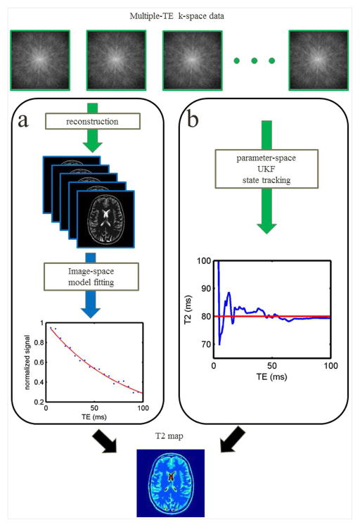
Moderate acceleration factors of 2–4 can be achieved using conventional parallel imaging methods (9,10), but the intrinsic SNR penalty limits higher acceleration factors. Higher acceleration factors have been reported using compressed sensing methods (11) that enforce sparsity in k-space and p-space (12,13). One of the successful constraints for compressed sensing acceleration is model-based sparsity. This assumes that the image structures are similar for each measurement and signals from different pixels follow a similar evolution pattern in p-space. By enforcing sparsity in the domain of a T2 decay model, compressed sensing methods are used to recover images and improve T2 estimation. One approach recovers T2 weighted images by linearizing the T2 decay model. A dictionary is trained to represent T2 decay signals sparsely by a linear combination of only a few elements. This can be an orthogonal dictionary from principal component analysis (14) or an over-complete dictionary obtained using the K-SVD technique (8). Most of these methods estimated T2 map in two steps: reconstruction of T2 weighted images from k-space data, followed by regression of the T2 map pixel by pixel in image space (Fig. 1a).
Fig. 1.
T2 mapping paradigms. With multiple-TE measurements, a T2 map is conventionally processed as shown in (a). k-space data are reconstructed to T2-weighted images. The intensity of each pixel (blue dots) is regressed to the signal decay model (red line) and results in the local T2 value. The proposed method (b) tracks the T2 value in parameter-space using the UKF, which produces the T2 map from the k-space data directly. The red line indicates the true T2 value. The blue line illustrates the tracking process, which approaches the true T2 value as more measurements are included.
High acceleration factors can also be achieved by nonlinear inversion of the measurement function (15,16). These studies employed the conjugate gradient method to pursue the parameter map, where a nonlinear T2 decay model was solved as data fidelity term. This approach has two drawbacks: first, the nonlinear inversion is computationally complex when using multiple TE measurements; second, it requires regularization constraints to avoid noise amplification during iteration, which would otherwise limit accuracy.
In MRI, we do not measure the T2 map directly, but rather Fourier-encoded images that are nonlinear functions of local T2. Each acquired signal corresponds to samples of the T2 map in combined k-p-space. When we use multiple TEs to sample the signal decay curve, we are observing T2 in k-p-space at multiple encoding states. This is similar to the process of tracking the location of a moving object by multiple detectors. This viewpoint suggests that it should be possible to track the parameter of interest, T2, by considering it as the state of a dynamic process, while modeling k-p-space sampling using a measurement function related to this dynamic process (Fig. 1b).
The Kalman filter has been widely used in state tracking and parameter estimation. It is an efficient optimal estimator that uses the previous measurements to estimate the current state recursively. Recently, Sümbül et al. (17) and Feng et al. (18) successfully adapted it to dynamic MRI by exploiting spatial and temporal redundancy. As our prior work has shown (19), in parameter mapping, we can treat the parameter map as the state of a dynamic system, model the parameter encoding and Fourier encoding steps in one measurement function, and use the Kalman filter to improve our estimate as more measurements are introduced. The classic Kalman filter is linear; for a nonlinear problem such as this, the unscented Kalman filter (UKF) (20) can be used to represent the non-linear measurement with third order accuracy.
The goal of this work was to explore a paradigm of state tracking for parameter mapping, which can provide optimal parameter estimation. An unscented Kalman filter based on a T2 decay model was applied to accelerate T2 mapping in combination with parallel imaging. The proposed method was compared with a nonlinear inversion reconstruction using a numerical phantom and retrospectively undersampled volunteer data. Finally, an accelerated pulse sequence was developed to undersample k-p-space prospectively.
Methods
Kalman filter
The Kalman filter (21) is a recursive and efficient method for estimating the state of a system from noisy measurements, and it is optimal in the maximum likelihood sense for a Gaussian noise model. The Kalman filter describes a dynamic system using two equations: the state transition equation describes the evolution of the underlying system, and the measurement equation describes how the measurements of the system are related to the system state. The system state is updated recursively based on the measurements. The general Kalman filter can be expressed as follows:
| [1] |
where f is the state transition function; xk is the kth state of system.; wk−1 is the system noise, assumed to be white Gaussian noise with covariance matrix Q; h is the measurement function of state xk; zk is the measured data; vk is the measurement noise, also assumed to be white Gaussian noise with covariance matrix R; and k is the state index.
T2 Decay model in the Kalman filter
For the special case of T2 mapping, we observe the signal decay at a rate of T2 in p-space. Here we choose the T2 map as the system state, which is assumed to be constant in time, and let k be the index of each TE measurement. Therefore, the state transition function is
| [2] |
The measurement function h(xk, vk) describes the relationship between T2 and the acquired signal:
| [3] |
where Uk is an undersampling pattern at the kth state, F is a Fourier transform operator and S is a coil sensitivity map. M(tk, xk) is the T2 weighted image at the kth state:
| [4] |
where tk is the echo time.
With constant echo spacing, the T2 weighted signal can be simplified as follows:
| [5] |
Here, we treat the shortest TE measurement from k = 1, so M(1) = ρe−Δt/T2. When the shortest TE is equal to the echo spacing Δt, ρ is then a proton density image. When the shortest TE is longer than Δt, ρ is a T2 weighted image. K is the echo train length.
Given the state transition function f and measurement function h, the Kalman filter estimation problem is now defined. The system state xk -- the desired T2 map -- can be estimated by the UKF, as described in the following section.
Unscented Kalman Filter
The basic Kalman filter uses linear state transition and measurement functions. It can be adapted to nonlinear models using various approximations. An early version of this approach was the extended Kalman filter (EKF), which linearizes the filter using a Jacobian matrix. The EKF has limited accuracy for highly nonlinear problems. The unscented Kalman filter represents the nonlinear model by the unscented transform, follows the state distribution using a deterministic sampling approach and achieves higher order approximation of the measurement.
The main difference between the UKF and the conventional Kalman filter is that the UKF does not use the T2 map directly in the tracking process, but instead generates a series of states around the target T2 state to represent its behavior in the dynamic system. This series of states are called sigma vectors χi and they are generated according to the variance of the T2 state:
| [6] |
where N is the dimension of the T2 state and Ti is the ith column of the matrix square root of the covariance matrix (N + λ)Pk−1:
| [7] |
λ is a scaling factor and α =0.01 describes the distance between xk−1 and the generated sigma vectors:
| [8] |
As with xk−1, the sigma vectors χk−1,i propagate from the previous TE measurement to the current TE measurement by the function f:
| [9] |
Each sigma vector χk,i is measured, which yields the k-space signal ζk,i:
| [10] |
The estimated state is represented by a combination of the current sigma vectors:
| [11] |
The measured signal z is estimated by a combination of ζ:
| [12] |
where
| [13] |
The difference between the acquired data zk and estimated data is updated to correct the prediction in the next state xk:
| [14] |
G is the gain matrix and it is expressed as
| [15] |
where
| [16] |
| [17] |
| [18] |
β describes the prior knowledge of x. β = 2 is optimal for a Gaussian distribution (22).
The covariance matrix Pk estimates the error of current state xk:
| [19] |
| [20] |
The above steps (Eqs. 6–20) proceed recursively until all the measurements are included.
Two parameter estimation
We will refer to the above method as the single-parameter UKF method, because it estimates a T2 map with the assumption that ρ is known. A pre-scan to obtain a ρ map is feasible, but this requires additional scan time and could introduce measurement error. We can incorporate ρ into the estimated state, doubling the number of variables to be estimated and increasing the computational complexity. We will simply refer this two-parameter UKF method as the UKF method in following parts of this paper. In the UKF method, Eq. 2 becomes:
| [21] |
As for the single-parameter UKF method, we assume the minimum TE map ρ is constant in time.
Parameter initialization
To reduce the size of the covariance matrix in the calculations, we first localize the image pixels using a 1D Fourier transform along the readout direction, as in Feng et al. (18). The minimum TE weighted ρ map is initialized by the measurement with the shortest TE in the UKF method. The T2 map is empirically initialized to a constant value, such as 80 ms.
Here we assume the estimated T2 map is real and the phase information is included in sensitivity maps, as in parallel image reconstruction with SENSE (9). Sensitivity maps can be estimated from low resolution images or a calibration scan. In the current method, we assume sensitivity maps are provided as prior knowledge; a discussion of how to estimate an accurate sensitivity map is beyond the scope of this work.
The initial estimation error covariance matrix P0 is empirically chosen as a diagonal matrix proportional to the noise level σ2 of the measured image, and the matrix is updated with each TE measurement. The inaccuracy in P0 is thus corrected as more TE measurements are included.
The distribution of noise v is assumed to be a stationary process, which does not change during the scan. Its covariance matrix R becomes a diagonal matrix with each diagonal element equal to σ2I in the case of white Gaussian noise. This assumption is likely to be more reliable for T2 measurements of the brain than of the heart, because there is less motion and change in volume. To simplify the calculation, we assume that the noise from the multiple channels v1, …, vn follow the same distribution R. However, we empirically choose a small Q to stabilize the estimation. There should be little change between each state in T2. Tuning the parameters Q and R can improve the performance of the UKF.
Simulations
A realistic analytical phantom (23) was used to simulate the acquisition, reconstruction and parameter estimation process. We divided the brain into four regions-of-interest (ROIs) with T2s of 50, 80, 120 and 250 ms. The proton density M0 was normalized to 1. To simulate the multiple-TE measurements, 70 parameter encoding states were generated with echo spacing equal to 5 ms. These images were sampled by a Cartesian trajectory with a matrix size of 128×128 with receiver phase following the Biot-Savart law (23). The generated data was contaminated by additive white Gaussian noise. SNR was defined according to the T2 weighted image with the shortest TE measurement.
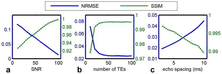
To evaluate the sensitivity of the proposed method to changes in experimental conditions, we evaluated estimated T2 maps while varying the noise level, the number of echoes, and the echo spacing. For these simulations, the data was fully sampled. In the noise tolerance test, T2 mapping acquisitions were simulated with echo spacing 5 ms, 70 echoes, and SNR varying from 10 to 100. In the test of the number of echoes, the acquisitions were simulated with SNR 50, echo spacing 5 ms, and the number of echoes varying from 10 to 100. In the test of echo spacing, the acquisitions were simulated with SNR 50, 32 echoes, and echo spacing varying from 3 ms to 10 ms.
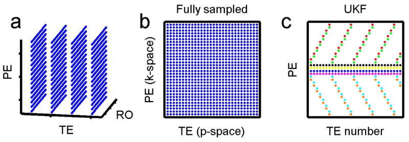
To verify the performance of UKF methods with an accelerated acquisition, we retrospectively undersampled k-space by factors of 2, 4, 6, and 8 at each TE. Other parameters were SNR 50 and 70 echoes with echo spacing 5 ms. The proposed methods were compared to the nonlinear inversion method of Sumpf et al. (16), which uses a conjugate gradient (CG) method to perform the inversion. The same sensitivity map was provided as prior knowledge for CG and the proposed method. Both methods used the same undersampling pattern. As shown in Fig. 2c, the undersampling pattern includes a few central phase-encoding lines and a few outer k-space lines at each TE. This pattern is designed to contain the same number of phase encoding lines at each TE value, so that it is compatible with a multiple-contrast spin echo pulse sequence. Each color of dot represents data that is acquired during a single echo train.
Fig. 2.
T2 data sampling patterns in k-p-space. (a) and (b) show fully sampled patterns in k-p-space. Data is always fully sampled in the readout direction. (c) Undersampling pattern for the UKF with acceleration rate 4. Each color of dots indicates phase encoding lines that are collected during the same echo train when using the accelerated pulse sequence. Four of the echo trains (black, yellow, blue, and pink dots) collect fully-sampled data at the center of k-space by collecting the same phase encoding at each echo. The other four echo trains collect undersampled data in the outer region of k-space, cycling through a set of phase encodings.
At SNR 50 (σ = 0.02), one hundred realizations of k-space were performed for Monte Carlo simulations. Independent and identically distributed complex Gaussian noise was generated and added to the k-space data. Each data set was undersampled with acceleration factors 2, 4, 6 and 8, and reconstructed by the proposed method and Sumpf’s CG method.
The results were compared with the fully sampled noiseless T2 map and quantified by the structural similarity index (SSIM) (24) and the normalized root of mean squared error (NRMSE).
Experiments
T2 mapping data with multiple TE measurements were acquired on normal volunteers. All of the experiments were performed on a 3T Siemens Trio scanner with a 12-channel head coil. The study followed a human subject protocol approved by the University of Virginia with written informed consent from each subject.
A modified multiple-contrast spin echo sequence was used to acquire fully sampled data. Each phase encoding was acquired in one echo train at different TEs. The parameters were as follows: TR 2.5 s, slice thickness 5 mm, FOV 220 mm, matrix size 192 × 192, bandwidth 500 Hz/pixel, 70 spin echoes, and echo spacing of 5.5 ms. The total scan time was approximately 8 minutes.
The volunteer data was retrospectively undersampled by factors of 2, 4, 6 and 8 with the same undersampling scheme used for the simulation. The signal from the first echo was not used, to avoid transient signal variation. We estimated the sensitivity map by combining undersampled data from multiple echoes (16). The UKF method and CG method were used to estimate the T2 and ρ maps. The results were evaluated using SSIM and NRMSE by comparison to the standard T2 map, which was obtained from fully sampled data and least squared error model fitting. Gray matter (T2 < 90 ms) and white matter (T2 = 90–150 ms) ROIs were defined to evaluate the relative performance of the methods in these regions.
To accelerate the acquisition, we adapted the undersampling scheme into a multiple contrast spin echo sequence to achieve prospective undersampling. After excitation, the sequence collected 70 spin echoes with echo spacing of 5 ms, with each echo designed to acquire a phase encoding value selected according to the undersampling scheme. For example, the first echo train collected the highest line in each k-space cluster, shown as the red dots in Fig. 2c. The second echo train collected the green dots and third echo train collected the black dots, and so on. Three experiments were performed: one collected fully sampled k-space and the other two were undersampled prospectively by factors of 4 and 8. Other scan parameters were as follows: TR 2 s, slice thickness 5 mm, FOV 200 mm × 200 mm and image matrix size 128 × 128. With fully sampled k-space, the scan time would have been more than 4 minutes. With the accelerated sequence, the scan times were reduced to about 1 minute and 30 seconds for undersampling factors of 4 and 8, respectively. The sensitivity map was estimated from undersampled data as above and T2 maps were estimated by CG and UKF methods.
The image reconstruction was performed in MATLAB 2012b (The MathWorks, Inc) with a 4x GTX 680 Workstation (Amax Information Technologies, Inc). 12 CPU cores (Intel Xeon E5-2640 2.50GHz Processor LGA2011) were used for parallel computation.
Results
Simulations
The accuracy of T2 estimation strongly depends on the SNR of the acquired signal. Compared with the noiseless T2 map, the results in Fig. 3a show that the estimated T2 map has reduced error and increased similarity as the SNR of the acquisition increases. The amount of available data is also essential to the quality of estimation. As shown in Fig. 3b, as the number of TE measurements increases, estimation errors are reduced and structural similarity is increased. Acquiring more than 70 TE measurements yields limited improvement in T2 map quality, so we used 70 echoes for the experiments. Figure 3c shows the results with different echo spacing. With constant echo train length, larger echo spacing resulted in longer TE and lower SNR in the late echoes. Therefore, larger echo spacing reduced image quality and the accuracy of T2 estimation, resulting in lower SSIM and higher NMRSE.
Fig. 3.
Performance of the UKF method as a function of SNR, number of echoes and echo spacing.
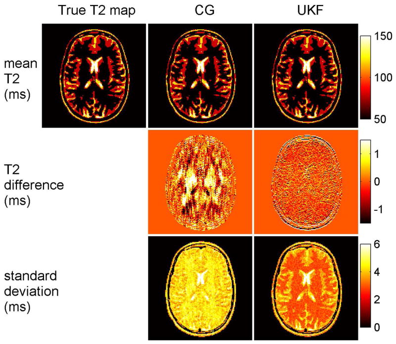
Figure 4 shows the results of Monte Carlo simulations of T2 mapping with the nonlinear inversion method and the UKF method. With an acceleration rate of 8, the mean T2 maps (top row) from 100 Monte Carlo simulations had negligible artifacts. The middle row shows the difference between the ‘true’ T2 map and the mean T2 maps of the two methods. The two methods have similar mean T2 values and these values are close to those of the true T2 map, which demonstrates that both methods are accurate. There is little spatial blurring of the mean maps with either method. The standard deviation of the estimated T2 maps (bottom row) show that the UKF method resulted in more stable results than the nonlinear inversion method and thus more precise estimation of T2.
Fig. 4.
T2 estimation in Monte Carlo simulations with the nonlinear inversion method and the UKF method. Top row: True T2 map and the mean T2 maps from 100 Monte Carlo simulations of the two methods with an acceleration rate of 8. Middle row: Difference between true T2 map and mean T2 maps of Monte Carlo simulations. Bottom row: Standard deviation of the Monte Carlo simulations for the two methods. The color bar indicates T2 and standard deviation in ms. Both methods demonstrate good accuracy and minimal blurring, and the UKF method has superior precision.
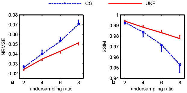
Figure 5 plots the quantitative results of the nonlinear inversion reconstruction and the proposed UKF method at acceleration factors of 2–8. Results are shown as the mean and standard deviation (×5) of the Monte Carlo simulations. The proposed method resulted in lower NRMSE error and higher similarity index. The proposed method also provided more stable performance with lower variance, as shown by the error bars.
Fig. 5.
Quantification of the error in the estimated T2 maps in simulation. With acceleration rates of 2, 4, 6 and 8, the UKF estimation results in lower NRMSE (left) and higher similarity index (right). It also provided stable performance with lower variance (×5).
Table 1 shows the mean NRMSE of the Monte Carlo simulations in four different ROIs with differing T2 values. As the acceleration rate (R) increased, the T2 estimation error increased in all ROIs, as expected. For each ROI and each acceleration rate, the proposed UKF method resulted in lower mean NRMSE than the CG method. The regions with shorter T2 values had higher mean normalized error with both methods.
Table 1.
Mean NRMSE of Monte Carlo simulations in four different ROIs with differing T2 values.
| ROI(T2) | R=2 | R=4 | R=6 | R=8 | |
|---|---|---|---|---|---|
| 250ms | UKF | 0.0173 | 0.0250 | 0.0306 | 0.0372 |
| CG | 0.0182 | 0.0260 | 0.0327 | 0.0394 | |
| 120ms | UKF | 0.0178 | 00256 | 0.0317 | 0.0387 |
| CG | 0.0186 | 0.0269 | 0.0334 | 0.0416 | |
| 80ms | UKF | 0.0209 | 0.0305 | 0.0378 | 0.0465 |
| CG | 0.0223 | 0.0328 | 0.0414 | 0.0521 | |
| 50ms | UKF | 0.0270 | 0.0395 | 0.0494 | 0.0593 |
| CG | 0.0297 | 0.0460 | 0.0620 | 0.0839 |
Experiments
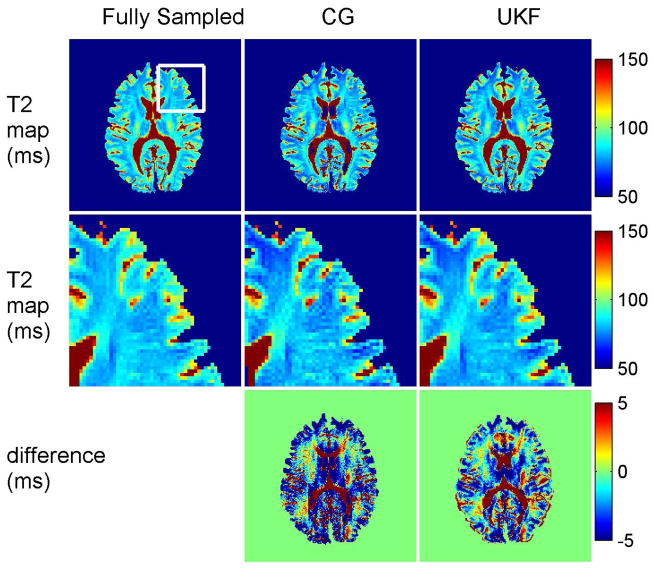
Volunteer results with retrospective undersampling are shown in Fig. 6. As in simulation, the UKF method estimated the T2 map accurately, based on comparison with fully sampled data. At an acceleration rate of 4, T2 maps from both methods had lower SNR and more error at the interfaces between cerebrospinal fluid and gray matter. The two methods show estimation errors in similar regions, which could be partly due to errors in the sensitivity map estimation. The map estimated with the CG method (NRMSE = 0.0544) had noticeable noise, as shown in the zoomed-in images along the middle row. The map estimated with the UKF method had negligible artifacts and lower estimation error (NRMSE = 0.0425) than the CG method.
Fig. 6.
Top row: T2 maps from the nonlinear inversion method and the UKF method from a volunteer scan. Middle row: Zoomed-in views of the maps. With a retrospective undersampling factor of 4, the expected loss of SNR was the principal difference with the fully sampled map. The two methods resulted in similar regions of estimation error, but the nonlinear inversion method resulted in higher estimation error. Bottom row: Error maps calculated by comparison with fully sampled data. The color bars for the T2 and error maps are in ms.
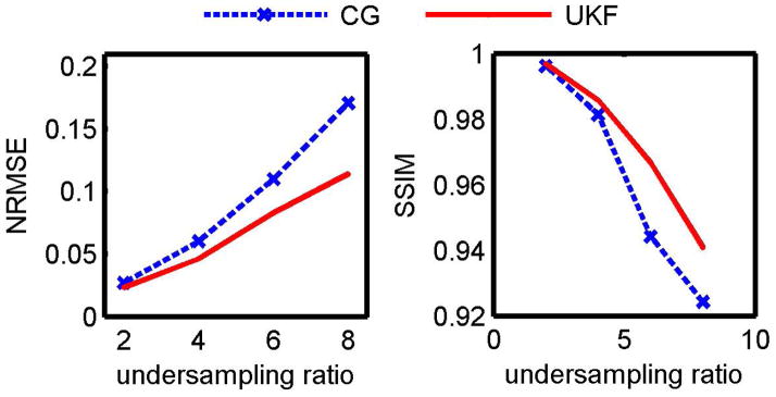
Quantitative metrics of the retrospectively undersampled T2 maps are shown in Fig. 7. As the acceleration rate increased, the estimation errors increased and structural similarity decreased. The UKF method resulted in lower NRMSE and higher SSIM at each level of undersampling.
Fig. 7.
Estimation errors with retrospectively undersampled volunteer data. The UKF method resulted in more accurate estimation than the nonlinear inversion method with lower NRMSE (left) and higher SSIM (right).
Table 2 shows the NRMSE in gray matter (GM) and white matter (WM) ROIs. As in simulation, as the acceleration rate increased, the T2 estimation error increased using each method. For each region and each acceleration factor, the proposed UKF method resulted in lower NRMSE than the CG method. For each method, the WM region had somewhat higher error than the GM region, except for R = 8. This is generally consistent with the simulation results that showed higher error in regions with shorter T2.
Table 2.
NRMSE of experimental T2 maps in gray matter (GM) and white matter (WM) regions.
| ROI | R=2 | R=4 | R=6 | R=8 | |
|---|---|---|---|---|---|
| GM | UKF | 0.0199 | 0.0394 | 0.0764 | 0.1134 |
| CG | 0.0231 | 0.0478 | 0.0903 | 0.1736 | |
| WM | UKF | 0.0211 | 0.0437 | 0.0813 | 0.1118 |
| CG | 0.0252 | 0.0567 | 0.1070 | 0.1470 |
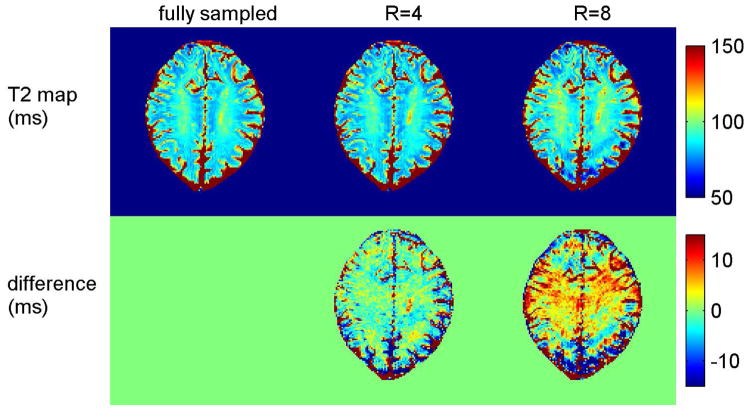
Figure 8 shows T2 maps from accelerated acquisitions with the undersampled sequence. The two-parameter UKF method recovered T2 maps with undersampling factors of 4 (Fig. 8, center) and 8 (Fig. 8, right). Compared to the T2 map from fully sampled k-p-space (Fig. 8, left), the proposed method has lower SNR as expected, but few aliasing artifacts.
Fig. 8.
The performance of the UKF method with accelerated acquisition. Compared with the T2 map from fully sampled k-space data (left), T2 maps and difference maps of UKF method are shown with acceleration rate 4 (middle) and acceleration rate 8 (right). The color bars for the T2 maps and error maps are in ms.
Discussion
In this work, we applied an unscented Kalman filter method to estimate parameter maps directly from highly undersampled k-space data. The method poses parameter mapping as a state-tracking problem in k-p-space. It uses MR parameters as the fundamental state space and the MR signal model as the measurement model. By monitoring the propagation of this dynamic system, the method yields quantitative parameter maps directly without image reconstruction. The method was applied to T2 mapping with undersampled k-space data. It achieved high accuracy in parameter estimation with undersampling factors of 2, 4, 6 and 8. The method yielded higher precision in simulation and experiment than a direct nonlinear inversion reconstruction. The proposed method was adapted into a multiple-contrast spin echo sequence and achieved prospectively accelerated acquisition.
The proposed method was applied to T2 map estimation in this study, but it could be applied to other parameter mapping problems, such as T1 mapping with a Look-Locker pulse sequence and T2* in functional MRI (25). Since the Fourier transform operator is linear, the nonlinearity of the signal model prior to the Fourier transform is the main limit on the performance of the UKF estimator. While this was not a significant limitation for T2 mapping, it could be more of a limitation for other parameter estimation problems, such as perfusion-weighted imaging.
The proposed method can be used to estimate multiple parameters of a model simultaneously, as demonstrated by the two-parameter UKF method, where both T2 and ρ were estimated. However, a more complex model could reduce the accuracy of estimation and require more measurements.
The accuracy of parameter estimation is limited by the number of measured states in p-space. The Kalman filter yields the maximum likelihood estimate, which approaches the minimum variance estimate when the number of encoding states is large enough. Acquiring more measurements along p-space increases the estimation accuracy. However, the number of TE measurements in a multiple contrast spin echo sequence is limited by the readout bandwidth and SNR. The measurements with long TE are noisy and yield limited improvement of the estimate. The number of measurements in p-space can also be limited by the specific application and available scan time.
An alternate way to improve estimation accuracy is to improve the convergence of the UKF estimator. The first few iterations of a Kalman filter train the covariance P. A small initial P0 can stabilize the propagation of the covariance matrix P and can also constrain the estimated values to be near the initial values. More accurate initialization of the T2 and ρ could help with convergence, although this may slow down the training of the covariance matrix.
The directly estimated T2 map is a real image, rather than a complex image as in conventional image reconstruction. Here, we assumed that the phase of the image is contained in the sensitivity maps and is constant with TE, so that the phase of the images at different echo times can be removed and later recovered using the sensitivity maps. When using multiple channel data, the UKF method adopts the features of SENSE parallel image reconstruction, which helps to improve the quality of the estimated parameter map. In a single coil measurement, the proposed method still performs better with a sensitivity map, because it provides phase information for data fidelity. The accuracy of the sensitivity map will directly affect the accuracy of the estimated T2 map. At high acceleration rates, it is difficult to estimate the sensitivity map accurately, which may result in bias in the T2 map. It should be possible to add sensitivity estimation to the UKF model, which would enable simultaneous estimation of a sensitivity map and a T2 map. However, this would also significantly increase the estimation complexity.
The accuracy of the estimated T2 map also depends on pulse sequence design. The multiple contrast spin echo sequence is time efficient compared to a conventional spin echo sequence, but acquired signal includes multiple signal pathways, which mixes stimulated echoes and indirect echoes (26–28). The accuracy is also limited by the performance of the refocusing RF pulses (29). Therefore, the T2 signal is not accurately modeled by a mono-exponential T2 decay model. Inaccuracy in the signal model could result in bias in T2 estimation. Additionally, in fully sampled k-p-space, the same phase encoding lines are acquired in one excitation, but in undersampled k-p-space some of the phase encoding lines are acquired in different echo trains. The order of phase encoding lines could introduce more variation in the quantification of the T2 map. In this work, our main focus was on the design of the parameter tracking algorithm, and additional improvements are possible with better sequence design.
The 1D simplification achieved by performing a 1D Fourier transform along the readout direction before the UKF reduces the size of the error covariance matrix P and improves the memory efficiency of the calculation. However, it also reduces the correlation information between different phase encoding lines, and thus does not capitalize on some potential improvements in estimation accuracy. Without using this 1D simplification, the proposed method can be adapted to other trajectories, such as spiral and radial, with a nonuniform Fourier transform F in Eq. [3].
The proposed method computes T2 maps directly, without reconstructing T2-weighted images. For applications that require such images, a T2-weighted image can be generated based on the resulting T2 and ρ maps.
The performance of compressed sensing strongly depends on the undersampling pattern, and this is also true for UKF and Sumpf’s CG methods. We used simple undersampling patterns in this work. An optimal undersampling pattern design could improve the performance of both the UKF and CG methods, but this is beyond the scope of this paper. In this work, the UKF method proved to be more precise than the nonlinear inversion method, but more work is needed to determine whether this will be true in general. At a minimum, this work demonstrates that established methods of state tracking can be competitive with nonlinear inversion methods for MR parameter estimation. Much of the power of both classes of methods rests on their ability to incorporate prior information.
Conclusion
In this work, we described a new paradigm for parameter mapping based on the unscented Kalman filter. This method estimates the parameter map directly from the k-p-space data and provides accurate estimation of T2 maps at high acceleration factors.
Acknowledgments
Grant support: NIH R01 HL079110, Siemens Medical Solutions
The authors would like to thank Dr. John P. Mugler, III and Dr. Samuel W. Fielden for their help with pulse sequences.
References
- 1.Chan I, Wells W, Mulkern RV, Haker S, Zhang J, Zou KH, Maier SE, Tempany CMC. Detection of prostate cancer by integration of line-scan diffusion, T2-mapping and T2-weighted magnetic resonance imaging; a multichannel statistical classifier. Med Phys. 2003;30:2390–2398. doi: 10.1118/1.1593633. [DOI] [PubMed] [Google Scholar]
- 2.Oh J, Cha S, Aiken AH, Han ET, Crane JC, Stainsby JA, Wright GA, Dillon WP, Nelson SJ. Quantitative apparent diffusion coefficients and T2 relaxation times in characterizing contrast enhancing brain tumors and regions of peritumoral edema. J Magn Reson Imaging. 2005;21:701–708. doi: 10.1002/jmri.20335. [DOI] [PubMed] [Google Scholar]
- 3.Siemonsen S, Mouridsen K, Holst B, Ries T, Finsterbusch J, Ostergaard L, Fiehler J, Thomalla G. Quantitative T2 values predict time from symptom onset in acute stroke patients. Stroke. 2009;40:1612–1616. doi: 10.1161/STROKEAHA.108.542548. [DOI] [PubMed] [Google Scholar]
- 4.Giri S, Chung Y-C, Merchant A, Mihai G, Rajagopalan S, Raman SV, Simonetti OP. T2 quantification for improved detection of myocardial edema. J Cardiovasc Magn Reson. 2009;11:56. doi: 10.1186/1532-429X-11-56. [DOI] [PMC free article] [PubMed] [Google Scholar]
- 5.Baudrexel S, Nürnberger L, Rüb U, Seifried C, Klein JC, Deller T, Steinmetz H, Deichmann R, Hilker R. Quantitative mapping of T1 and T2* discloses nigral and brainstem pathology in early Parkinson’s disease. Neuroimage. 2010;51:512–520. doi: 10.1016/j.neuroimage.2010.03.005. [DOI] [PubMed] [Google Scholar]
- 6.Dai W, Robson PM, Shankaranarayanan A, Alsop DC. Reduced resolution transit delay prescan for quantitative continuous arterial spin labeling perfusion imaging. Magn Reson Med. 2012;67:1252–1265. doi: 10.1002/mrm.23103. [DOI] [PMC free article] [PubMed] [Google Scholar]
- 7.Liu F, Chaudhary R, Hurley SA, Samosonov A, Alexander A, Deoni SC, Block WF, Kijowski R. Multi-Component T2 Analysis of Cartilage Degradation Model Using mcDESPOT at 3.0T. Proc. Sci. Meet. Int. Soc. Magn. Reson. Med; 2013; p. 1655. [Google Scholar]
- 8.Doneva M, Börnert P, Eggers H, Stehning C, Sénégas J, Mertins A. Compressed sensing reconstruction for magnetic resonance parameter mapping. Magn Reson Med. 2010;64:1114–1120. doi: 10.1002/mrm.22483. [DOI] [PubMed] [Google Scholar]
- 9.Pruessmann KP, Weiger M, Scheidegger MB, Boesiger P. SENSE: sensitivity encoding for fast MRI. Magn Reson Med. 1999;42:952–962. [PubMed] [Google Scholar]
- 10.Griswold MAa, Jakob PMM, Heidemann RMM, Nittka M, Jellus V, Wang J, Kiefer B, Haase A. Generalized autocalibrating partially parallel acquisitions (GRAPPA) Magn Reson Med. 2002;47:1202–1210. doi: 10.1002/mrm.10171. [DOI] [PubMed] [Google Scholar]
- 11.Lustig M, Donoho D, Pauly JM. Sparse MRI: The application of compressed sensing for rapid MR imaging. Magn Reson Med. 2007;58:1182–1195. doi: 10.1002/mrm.21391. [DOI] [PubMed] [Google Scholar]
- 12.Zhang T, Pauly JM, Levesque IR. Accelerating Parameter Mapping with a Locally Low Rank Constraint. 2014;00:1–7. doi: 10.1002/mrm.25161. [DOI] [PMC free article] [PubMed] [Google Scholar]
- 13.Velikina JV, Alexander AL, Samsonov A. Accelerating MR parameter mapping using sparsity-promoting regularization in parametric dimension. Magn Reson Med. 2013;70:1263–1273. doi: 10.1002/mrm.24577. [DOI] [PMC free article] [PubMed] [Google Scholar]
- 14.Huang C, Graff CG, Clarkson EW, Bilgin A, Altbach MI. T2 mapping from highly undersampled data by reconstruction of principal component coefficient maps using compressed sensing. Magn Reson Med. 2012;67:1355–1366. doi: 10.1002/mrm.23128. [DOI] [PMC free article] [PubMed] [Google Scholar]
- 15.Block KT, Uecker M, Frahm J. Model-based iterative reconstruction for radial fast spin-echo MRI. IEEE Trans Med Imaging. 2009;28:1759–1769. doi: 10.1109/TMI.2009.2023119. [DOI] [PubMed] [Google Scholar]
- 16.Sumpf TJ, Uecker M, Boretius S, Frahm J. Model-based nonlinear inverse reconstruction for T2 mapping using highly undersampled spin-echo MRI. J Magn Reson Imaging. 2011;34:420–8. doi: 10.1002/jmri.22634. [DOI] [PubMed] [Google Scholar]
- 17.Sümbül U, Santos JM, Pauly JM. A practical acceleration algorithm for real-time imaging. IEEE Trans Med Imaging. 2009;28:2042–2051. doi: 10.1109/TMI.2009.2030474. [DOI] [PMC free article] [PubMed] [Google Scholar]
- 18.Feng X, Salerno M, Kramer CM, Meyer CH. Kalman filter techniques for accelerated Cartesian dynamic cardiac imaging. Magn Reson Med. 2012;69:1346–1356. doi: 10.1002/mrm.24375. [DOI] [PMC free article] [PubMed] [Google Scholar]
- 19.Zhao L, Meyer CH. Direct & accelerated parameter mapping using the unscented Kalman filter. Proc Intl Soc Mag Reson Med. 2014;22:3129. doi: 10.1002/mrm.25796. [DOI] [PMC free article] [PubMed] [Google Scholar]
- 20.Wan E, Van Der Merwe R, Nelson A. Dual Estimation and the Unscented Transformation. Neural Inf Process Syst. 2000:666–672. [Google Scholar]
- 21.Welch G, Bishop G. An Introduction to the Kalman Filter. Univ. North Carolina; 2001. [Google Scholar]
- 22.Wan EA, Van Der Merwe R. The unscented Kalman filter for nonlinear estimation. Proc. IEEE 2000 Adapt. Syst. Signal Process. Commun. Control Symp; 2000; pp. 153–158. [Google Scholar]
- 23.Guerquin-Kern M, Lejeune L, Pruessmann KP, Unser M. Realistic analytical phantoms for parallel magnetic resonance imaging. IEEE Trans Med Imaging. 2012;31:626–636. doi: 10.1109/TMI.2011.2174158. [DOI] [PubMed] [Google Scholar]
- 24.Wang Z, Bovik AC, Sheikh HR, Simoncelli EP. Image quality assessment: from error visibility to structural similarity. IEEE Trans Image Process. 2004;13:600–612. doi: 10.1109/tip.2003.819861. [DOI] [PubMed] [Google Scholar]
- 25.Olafsson VT, Noll DC, Fessler JA. Fast joint reconstruction of dynamic R2* and field maps in functional MRI. IEEE Trans Med Imaging. 2008;27:1177–1188. doi: 10.1109/TMI.2008.917247. [DOI] [PubMed] [Google Scholar]
- 26.Huang C, Bilgin A, Barr T, Altbach MI. T2 relaxometry with indirect echo compensation from highly undersampled data. Magn Reson Med. 2013;70:1026–37. doi: 10.1002/mrm.24540. [DOI] [PMC free article] [PubMed] [Google Scholar]
- 27.Ben-Eliezer N, Sodickson DK, Block KT. Rapid and accurate T2 mapping from multi-spin-echo data using Bloch-simulation-based reconstruction. Magn Reson Med. 2014;73:809–817. doi: 10.1002/mrm.25156. [DOI] [PMC free article] [PubMed] [Google Scholar]
- 28.Sumpf TJ, Petrovic A, Uecker M, Knoll F, Frahm J. Fast T2 mapping with improved accuracy using undersampled spin-echo MRI and model-based reconstructions with a generating function. IEEE Trans Med Imaging. 2014 Dec;33(12):2213–22. doi: 10.1109/TMI.2014.2333370. [DOI] [PMC free article] [PubMed] [Google Scholar]
- 29.Poon CS, Henkelman RM. Practical T2 quantitation for clinical applications. J Magn Reson Imaging. 1992;2:541–553. doi: 10.1002/jmri.1880020512. [DOI] [PubMed] [Google Scholar]


