Impact of Age, Race and Socio-economic Status on Temporal Trends in Late-Stage Prostate Cancer Diagnosis in Florida

Abstract

Individual-level data from the Florida Cancer Data System (1981–2007) were analysed to explore temporal trends of prostate cancer late-stage diagnosis, and how they vary based on race, income and age. Annual census-tract rates were computed for two races (white and black) and two age categories (40–65, >65) before being aggregated according to census tract median household incomes. Joinpoint regression and a new disparity statistic were applied to model temporal trends and detect potential racial and socio-economic differences. Multi-dimensional scaling was used as an innovative way to visualize similarities among temporal trends in a 2-D space. Analysis of time-series indicated that late-stage diagnosis was generally more prevalent among blacks, for age category 40–64 compared to older patients covered by Medicare, and among classes of lower socio-economic status. Joinpoint regression also showed that the rate of decline in late-stage diagnosis was similar among older patients. For younger patients, the decline occurred at a faster pace for blacks with rates becoming similar to whites in the late 90s, in particular for higher incomes. Both races displayed distinct spatial patterns with higher rates of late-stage diagnosis in the Florida Panhandle for whites whereas high rates clustered in South-eastern Florida for blacks.

1. Introduction

Racial inequalities in health care and health outcomes between blacks and whites are well documented. Compared to other major cancer sites, racial differences in incidence and mortality are the greatest for prostate cancer, with several studies reporting rates of late-stage diagnosis twice as high for blacks compared with non-Hispanic whites (Brawn et al., 1993; Hoffman et al., 2001). Common culprits behind the disparity in the stage at diagnosis include demographic characteristics (e.g. fewer married men), lower socioeconomic status, and higher prevalence and severity of comorbid conditions (e.g. congestive heart failure) which may limit cancer screening in the black population and contribute to a delayed diagnosis (Carpenter et al., 2010; Jones et al., 2008; Virnig et al., 2009). Several studies have also highlighted a difference in utilization of Health Services between blacks and whites (Musa et al., 2009; Do et al., 2010; Laiyemo et al., 2010). Regardless of race, lower income has been associated with a statistically significantly increased risk of distant-stage prostate cancer (Clegg et al., 2009; Robbins et al., 2000; Schwartz et al., 2003). In general, living in socioeconomically disadvantaged neighborhoods decreases the use of screening services (Hayanga et al., 2009; Xiao et al., 2014) because persons living in these neigborhoods are less likely to have health insurance (Ward et al., 2010). Another explanation is that racial differences in tumor biology, possibly attributable to differences in dietary, hormonal, or molecular factors, may lead to more aggressive tumors (Morton Jr, 1994).

According to Salinas et al. (2014), the incidence of prostate cancer in young men (age ≤ 55 years) increased by 5.7-fold between 1986 and 2008 (Salinas et al., 2014). These patients with early-onset prostate cancer were however more likely to have low-grade cancers than their older counterparts. Similarly, Bechis et al. (2010) found that older patients were more likely to have high-risk prostate cancer at diagnosis and less likely to receive local therapy (Bechis et al., 2011). Scosyrev et al. (2011) also reported that men aged 75 years and older were more likely to have advanced prostate cancer because of more aggressive disease (e.g. faster growing tumors) in the elderly and/or less frequent use of PSA testing and further diagnostic evaluation (such as biopsy for an elevated PSA) in older men compared with younger men (Scosyrev et al., 2012). None of these studies however looked at the interaction between age and race on the frequency of late-stage diagnosis.

Most of the above studies did not incorporate time in their analysis, and when they did 4-yr time periods instead of annual rates were used (e.g. Clegg et al., 2009). Prostate cancer mortality and late–stage diagnosis have however declined significantly in the last two decades, a decline that started mostly after 1991 (Chu et al., 2003; Smart, 1997). According to some studies, this decline in mortality is due to early detection (PSA screening) although screening for prostate cancer is still controversial (Andriole et al., 2009; Barratt & Stockler, 2009; Schröder et al., 2009; Wolf et al., 2010). In particular for Florida, state-level percentage of late-stage diagnosis decreased 50% since 1981; a decline that accelerated in the 90’s with increased use of prostate specific antigen (PSA) screening. Analysis at the metropolitan and non-metropolitan levels revealed that the frequency of late-stage diagnosis increased recently in urban areas, and this trend was significant for white males (Goovaerts & Xiao, 2011). The same authors showed that the annual rate of decrease in late-stage diagnosis and the onset years for significant declines varied greatly among counties and racial groups. Their analysis was however conducted at the county level, which precluded the use of socio-economic status as covariate.

The present study takes advantage of access to individual-level data to explore the impact of age, race and socio-economic status on proportions of prostate cancer late-stage diagnosis in Florida. Temporal trends are analyzed through the application of joinpoint regression (Kim et al., 2000) to annual time series spanning between 1981 and 2007. To visualize the impact of race and socio-economic status on temporal trends, we propose to project the ensemble of time series into 2D space using metric multi-dimensional scaling (MDS). The application of MDS to time series is fairly recent (Bernard et al., 2012) and applications to health data are rare (Lillo-Castellano et al., 2013). Two new metrics are here introduced to quantify the similarity between the magnitude and rate of changes of time series of health outcomes.

2. Data and Methods

Prostate cancer cases diagnosed between 1981 and 2007 were obtained from the Florida Cancer Data System (FCDS). The FCDS is part of the Centers for Disease Control and Prevention National Program of Cancer Registries (CDC-NPCR) and is nationally certified by the NAACCR at the highest level, gold certification. The original dataset included 321,640 cases with the following information: stage and age at diagnosis, year of diagnosis, race, and residential location when available (county, ZIP code, and 2000 census tract). Census tract information was missing for 24,100 cases, whereas 262 cases lack both ZIP code and census tract information. Geographical imputation (Henry & Boscoe, 2008; Sheehan et al., 2004) was used to allocate each of the 24,100 cases to a census tract based on the relative proportion of the ZIP code’s male population accounted for by each census tract for the decade when the case was diagnosed.

The present study focused on cases recorded for two races (white and black) and two categories of age (40–64, 65+). Out of the 321,640 original cases, 256,365 patients belonged to these categories of age and race, were successfully allocated to a census tract and their stage at diagnosis was known (Table 1). 2000’s census tract information was used to assign to each case an annual median household income.

Table 1.

Sample characteristics for each age group and race (average over 1981–2007).

Age group	Number of cases	Late stage (%)
White
40–64	50,463	17.91
65–120	180,624	16.99
Black
40–64	9,731	20.96
65–120	15,547	24.15

Individual-level data were processed to compute for each race and age category the census-tract proportion of late-stage diagnosis To create stable estimates, cases were aggregated into four time periods (1981–1989–1990–1994–1995–1999–2000–2007) which capture the situation before and after introduction of PSA screening in the early nineties. Instability caused by the small number problem was further reduced by the application of binomial kriging (Goovaerts, 2009) that borrows strength from neighboring census tracts for each time period.

Annual statewide proportions of late-stage diagnosis were also computed for the following five classes of annual median income that include equal proportions of census tracts: [0, $28,784], [$28,784, $34,760], [$34,760, $41,200], [$41,200, $51,838], and [$51,838, $200,000]. Joinpoint regression (Kim et al., 2009) and multidimensional scaling (Bernard et al., 2012) were conducted to visualize and analyze temporal trends at the State level and to detect potential racial and socio-economic differences.

The geostatistical filtering was applied using the commercial software SpaceStat 4.1 (BioMedware, 2013). Joinpoint regression was conducted using the public-domain Joinpoint Regression Program 4.1.1 August 2014 (Kim et al., 2000) developed at the US National Cancer Institute, NCI (http://surveillance.cancer.gov/joinpoint/). Multidimensional scaling (MDS) was performed using the procedure MDS in SAS 9.3 (SAS Institute Inc., 2011).

2.1. Binomial kriging

For a given number N of geographical units v_α (i.e. N=3,168 census tracts here), the observed proportion or rate of late-stage diagnosis is defined as z(v_α)=d(v_α)/n(v_α), where d(v_α) is the number of late-stage cases and n(v_α) is the total number of cases. Mapping the rates z(v_α) might lead to misleading conclusions since even after temporal aggregation most census tracts might include too few cases to compute reliable estimates of late-stage diagnosis rates, in particular for the minority group. The noise caused by the so-called “small number problem” can be filtered using the following estimator:

$$\widehat{r}(v_{\alpha })={\lambda }_{\alpha }z(v_{\alpha })+\sum _{i=1}^{K-1}{\lambda }_{i}z(v_i)$$ (1)

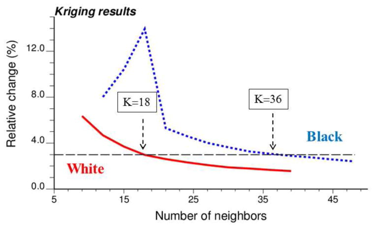
where the kernel rate z(v_α) is combined with rates observed in (K−1) neighboring entities v_i to borrow strength. In the present case-study, K=18 geographical units for white males to guarantee the use of a minimum of 16 cases across all census tracts and time periods. K was set to 36 units for black males because of the existence of fewer cases. The weights λ_i assigned to the K rates are computed by solving the following system of linear equations; known as “binomial kriging” system (Goovaerts, 2009; Webster et al., 1994):

$$\begin{array}{l}\sum _{j=1}^K{\lambda }_j\left[\overline{C}(v_i,v_j)+{\delta }_{ij}\frac{a}{n(v_i)}\right]+\mu (v_{\alpha })=\overline{C}(v_i,v_{\alpha })\mathrm{i}=1,\dots ,K\\ \sum _{j=1}^K{\lambda }_j=1.\end{array}$$ (2)

where δ_ij=1 if i=j and 0 otherwise, a = m*(1 − m*)−C̄_I(v_i, v_i), and m* is the population-weighted average of the N rates. The error variance term, a/n(v_i), accounts for variability arising from population size and it becomes larger as the number of cases n(v_i) decreases. Thus, its incorporation in the kriging system leads to smaller weights for less reliable rates based on fewer cases. The area-to-area covariance terms C̄(v_i, v_j) = Cov{Z(v_i),Z(v_j)} and C̄(v_i, v_α) are numerically approximated by averaging the point-support covariance C(h) computed between any two locations discretizing the census tracts v_i and v_j or v_α. The point-support covariance C(h), or equivalently the point-support semivariogram γ(h), are modeled from the data using a population-weighted estimator followed by an iterative deconvolution procedure (Goovaerts, 2008).

2.2. Joinpoint regression

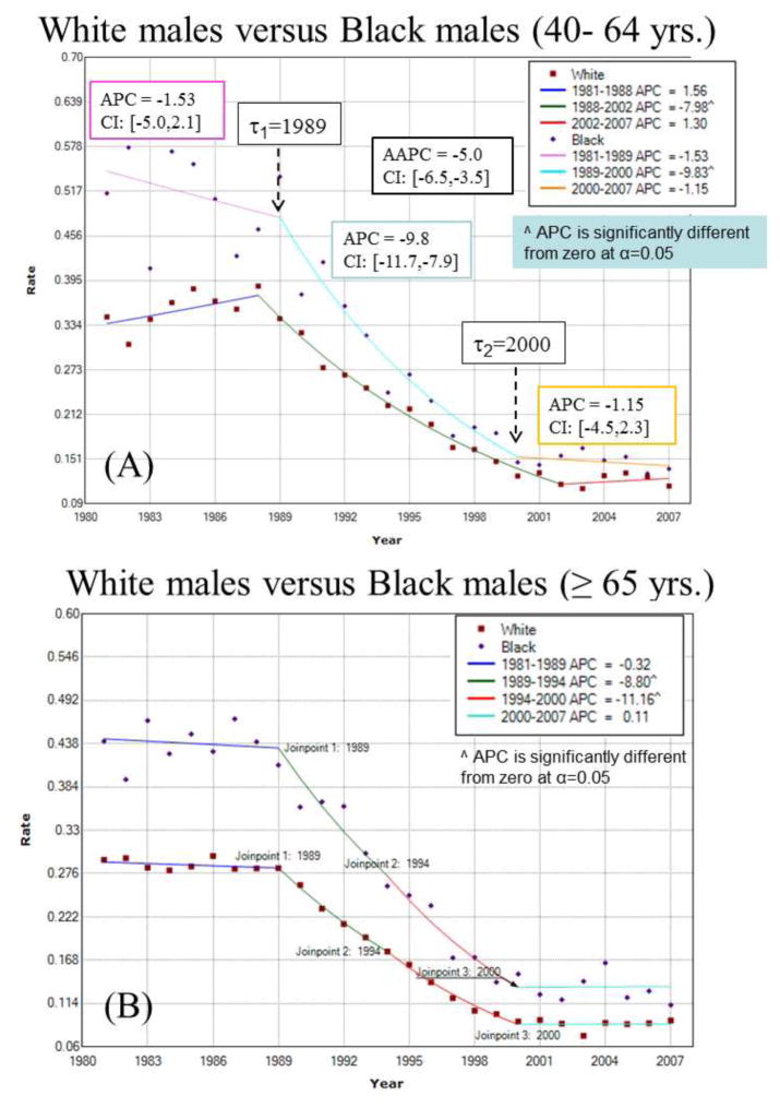
Let {z(c;t), t=1, …,T} be the proportions or rates of late-stage diagnosis recorded for category c (e.g. race, age or income class) at T different time periods (e.g. years). For example, Figure 1A (top curve) shows how the proportion of prostate cancer cases diagnosed late for black males in the [40,64] age bracket changed yearly between 1981 and 2007 (T=27). Joinpoint regression (Kim et al., 2000) models each time series as a sequence of linear segments. In its log-linear version, the segmented regression model for any class c is written as:

$$\text{Log}(z(c;t))=m(c;t)+\epsilon (c;t)t=1,\dots ,T$$ (3)

where ε(c;t) is the residual for the t-th time, and the regression mean m(c;t) is defined as a succession of (K(c)+1) linear segments (e.g. 3 segments in Figure 1A): [a,τ₁(c)] … (τ_k(c), τ_k+1(c)] … (τ_K(c),b]. The parameter τ_k(c) is the timing (joinpoint) for a statistically significant change in the slopes β_k(c) and β_k+1(c) of two successive segments.

Fig. 1.

Joinpoint regression model fitted to time series of proportion of late-stage prostate cancer cases for white and black males for two age categories: (A) 40 to 64 yr. old, and (B) 65 yr. and over. For example, the segmented regression model (solid line) for black males 40 to 64 yr. old includes two joinpoints (τ) that correspond to years of statistically significant changes in rate trend: 1989 and 2000. The estimate and 95% confidence intervals (CI) of the annual percent change (APC) are listed for each segment, as well as the average annual percent change (AAPC) computed for the entire time period. The hypothesis of parallelism of the two joinpoint regression models was rejected at α=0.05 for the youngest age bracket.

For example, the observed time series in Figure 1A (top curve) was fitted with a regression model that includes two joinpoints: τ₁=1989 and τ₂=2000. The rate did not change significantly until 1989 when it started declining at an annual pace of 9.8%. The decline stopped in 2000 and since then no significant change has been observed; see parameters listed in Figure 1A.

The unknowns in Equation (3) include the number and values of the joinpoints, as well as the regression parameters (e.g. slopes of linear segments). They are estimated using a two-step procedure: 1) a grid search method (Lerman, 1980)is conducted over the set of possible joinpoints, and 2) at each step of the search the regression parameters and their standard errors are estimated by weighted least-square regression using the following criterion:

$$Q={\sum }_{t=1}^{T}w(c;t){(log(z(c;t))-m(c;t))}^2$$ (4)

The weights account for the fact that the variance of the residuals ε(c;t) may vary with time (heteroscedasticity) as the number of cases changes. These weights were here defined as n(c;t)/[z(c;t)×(1-z(c;t))], which corresponds to the reciprocal of the variance for the Binomial distribution (Goovaerts & Xiao, 2011). Uncorrelated error models were considered since these are the only models available in the NCI software for testing the hypothesis of coincidence or parallelisms of different trend models.

The number K of joinpoints is estimated through an iterative procedure that tests whether models of increasing complexity (i.e. including more joinpoints) provide a significantly better goodness-of-fit than simpler models (Kim et al., 2009). The tests of significance use a Monte Carlo Permutation procedure described in (Kim et al., 2000). To reduce the number of solutions and the computational time, a maximum number of joinpoints is typically specified (i.e. K_max=3 here). A minimum number of observations between joinpoints (i.e. minimum length of linear segments) is also required and was set to 4 in the present study. This minimum number allowed the computation of the standard error of the slope parameters and the associated p-values.

Trends in health outcomes recorded for class c over time interval [τ_k(c), τ_k+1(c)] can be quantified by the annual percent change (APC) that is calculated from the slope of the regression model over that time interval as:

$${\mathit{APC}}_{k+\mathit{1}}(c)=100\times (exp\{{\beta }_{k+\mathit{1}}(c)\}-1)$$ (5)

Like other regression parameters, confidence intervals can be computed for each APC and one can test whether an APC is significantly different from zero (Kim et al., 2000). For the example of Figure 1A, the APC is particularly large for the period [1989, 2000]: the proportion of late-stage diagnosis declined around 9.8% per year. Changes were not significant outside this time period. The trend over the entire time series [a,b] can be summarized using the average annual percent change (AAPC) which is computed as the weighted average of the APC’s from the joinpoint model. The AAPC was −5.0% over the 25 year period.

Disparities in temporal trends for two classes c and c′ (e.g. two different races or age categories) can be detected by comparing the models fitted to their corresponding time series {z(c;t), t=1, …,T}and {z(c′;t), t=1, …,T}. Kim et al. (2004) proposed a permutation procedure to compare two segmented line regression functions and to test two types of hypothesis: 1) the two regression models are identical, or 2) the two mean functions are parallel allowing different intercepts (Kim et al., 2004). The first hypothesis is the most restrictive and implies that the two times series are similar both in terms of the magnitude of the health outcome (e.g. percentage of late-stage diagnosis) and their rate of change. The test of parallelism is less strict in that only the slopes and joinpoints are compared while the two time series can still display different intercepts; in other words one time series is the results of adding a constant (vertical shift) to the other one. Examples of application of the test of parallelism include the comparison of time series of breast cancer mortality rates for white females in Michigan and New York (Kim et al., 2004), or the analysis of time series of distant incidence rates and incidence based mortality rates for prostate cancer in the US (Wachtel et al., 2013).

In addition to these tests conducted globally over the entire time series, we conducted a finer comparison by computing for every time period t (i.e. year) the 95% confidence intervals of the APC for the two classes and counting the number of times these two intervals did not overlap. This disparity statistic introduced by Goovaerts and Xiao (2011) can be expressed as:

$$B_{c{c}^{\prime }}=\sum _{t=1}^{T}I(\text{CI}(c;t);\text{CI}(c^{\prime };t)){\sum }_{\mathrm{t}=1}^{\mathrm{T}}\mathrm{I}(\text{CI}({\mathrm{v}}_{\mathrm{\alpha }};\mathrm{t});\text{CI}({\mathrm{v}}_{{\mathrm{\alpha }}^{\prime }};\mathrm{t}))$$ (6)

where the indicator function I(.)=1 if the following condition on the upper bounds (U) and lower bounds (L) of the two confidence intervals CI are met: U(v_α; t) < L(v_α,; t) or L(v_α; t) > U(v_α,; t). A large number (i.e. B_cc′ → T) indicates that rates of changes for the two classes are consistently different over time. There is no statistical test associated with quantity B_cc′ which is mainly descriptive yet provides more information than the global tests of identity or parallelism that lack power when rates are computed from small number of cases.

2.3. Multidimensional scaling

Let {z(l;t), t=1, …,T; l=1,…,L} be a potentially large ensemble of L time series. The objective is to group time series based on the similarities in their temporal trends in order to detect any patterns in the ensemble. In this paper we adopted a distance-based approach to: 1) quantify differences between time series using two different and novel distance metrics (Euclidian versus APC-based distances), and 2) project the ensemble of time series into a low dimensional Cartesian space using multi-dimensional scaling (MDS) to better understand data structure, such as proximity between age groups versus racial groups.

The first step is to create a L×L distance matrix D whose elements d_ll′ measure the dissimilarity between any two time series {z(l;t), t=1, …,T}and {z(l′;t), t=1, …,T}. The following two novel metrics were considered in this study:

$$d_{l{l}^{\prime }}=\frac{1}{T}\sum _{t=1}^T\left[m(l;t)-m(l^{\prime };t)\right]$$ (7)

$$d_{l{l}^{\prime }}=\sum _{t=1}^{T}I(\text{CI}(l;t);\text{CI}(l^{\prime };t))=B_{l{l}^{\prime }}$$ (8)

Metric (7) is the average absolute differences between the trend models m(l;t) and m(l′;t) fitted by joinpoint regression. The second metric (Equation 8) quantifies differences in the annual percent change (APC) for the two time series and correspond to the disparity statistic described in Equation (6).

The second step takes the L×L matrix D and projects it onto a low N-dimensional space (with N < L) using the multi-dimensional scaling technique (MDS), also known as Principal Coordinate Analysis. MDS searches an orthogonal N-dimensional configuration of L points (one for each time series) such that dissimilarities among these points are as close as possible to the dissimilarities provided by the elements of the matrix D. In other words, if N=2, points close in the 2D space obtained by projection correspond to time series that display similar values (metric 1) or temporal trends (metric 2). Mathematically, the approach aims to find the N coordinates of a set of L points p_l such that the following stress criterion is minimum:

$$\mathit{STRESS}(N)=\sqrt{\frac{{\displaystyle \sum _{l=1}^L}{\displaystyle \sum _{l^{\prime }=1}^L}{\left(d_{l{l}^{\prime }}-\Vert {\mathbf{p}}_l-{\mathbf{p}}_{l^{\prime }}\Vert \right)}^2}{{\displaystyle \sum _{l=1}^L}{\displaystyle \sum _{l^{\prime }=1}^L}{d_{l{l}^{\prime }}}^2}}$$ (9)

where ||.||denotes the Euclidian norm. The MDS criterion will decrease with the number of dimensions N but at the expense of visualization which becomes challenging for more than three dimensions. The quality of the solution provided by MDS can be assessed visually through the Shepard diagram which is a scatterplot of the distances between points in the N-dimensional space (e.g. N=2) against the original dissimilarities d_ll′. The points in the scatterplot should adhere cleanly to a curve or straight line (Shepard, 1974). The goodness of fit can also be quantified using the amount of stress (Equation 9): a small stress value indicates a good fitting solution, whereas a high value indicates a bad fit. According to Kruskal (1964), a stress value lower than 0.05 indicates a good fit whereas the fit is poor if the stress exceeds 0.2.

3. Results and Discussion

3.1 Analysis of temporally averaged rates

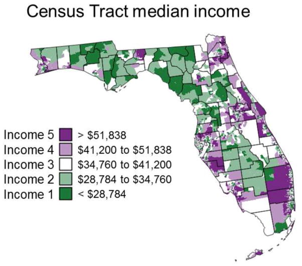
Table 1 indicates that on average over the State of Florida late-stage diagnosis was more prevalent for black males (21–24%) compared to white males (17–18%). The impact of age also differed between races with an increase in late-stage diagnosis for older black males while the reverse was observed for while males. The impact of socio-economic status on these results was investigated by assigning each cancer case to a category of income based on the 2000’s annual median household income for his census of residence. The five income classes, each including 20% of census tracts, are mapped in Figure 2. Regardless of racial and age category, the percentage of late-stage diagnosis displays a steady decline as the median household income grows from under $28,784 a year to above $51,838 (Table 2). The age-based ranking does not change across all five income classes: late-stage diagnosis is systematically more prevalent at younger age for white males and at older age for black males. Interestingly, racial disparities for patients in the age group [40, 65] disappear in affluent neighborhoods where the worst health outcomes are observed for older black males. The non-overlap of 95% confidence intervals (Table 2, italic) indicates the existence of significant racial differences only at the lowest income level for younger males and over all income classes for cases 65 years and older. Because fewer black males live in affluent neighborhoods, the corresponding confidence intervals grow wider compared to white males.

Fig. 2.

Census-tract level map of five categories of median household incomes that were used to explore the impact of socio-economic status on the proportions of late-stage prostate cancer cases diagnosed.

Table 2.

Percentages of late-stage prostate cancer cases diagnosed over the period 1981–2007 for five categories of median household income, two race groups (white and black males), and two age categories ([40–64], [65,120]). The lower and upper limits of the 95% confidence intervals were computed using the Gaussian approximation for binomial distributions and are reported in italic.

	Categories of median household income
Age group	[0,$28,784]	[$28,784,$34,760]	[$34,760,$41,200]	[$41,200,$51,838]	[$51,838,$200,000]
White
40–64	21.15	18.88	19.11	17.00	15.74
	20.1–22.2	18.1–19.7	18.4–19.9	16.3–17.7	15.1–16.3
65–120	19.25	17.57	17.67	16.34	14.31
	18.8–19.7	17.2–17.9	17.3–18.0	16.0–16.7	13.9–14.7
Black
40–64	25.37	20.41	19.64	16.98	13.77
	24.0–26.8	18.7–22.2	17.7–21.6	15.1–18.9	11.6–15.9
65–120	27.34	22.44	21.58	20.54	17.79
	26.3–28.3	20.9–24.0	19.9–23.3	18.7–22.4	15.4–20.1

3.2 Visualization of space-time trends

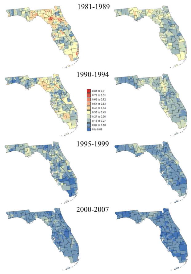
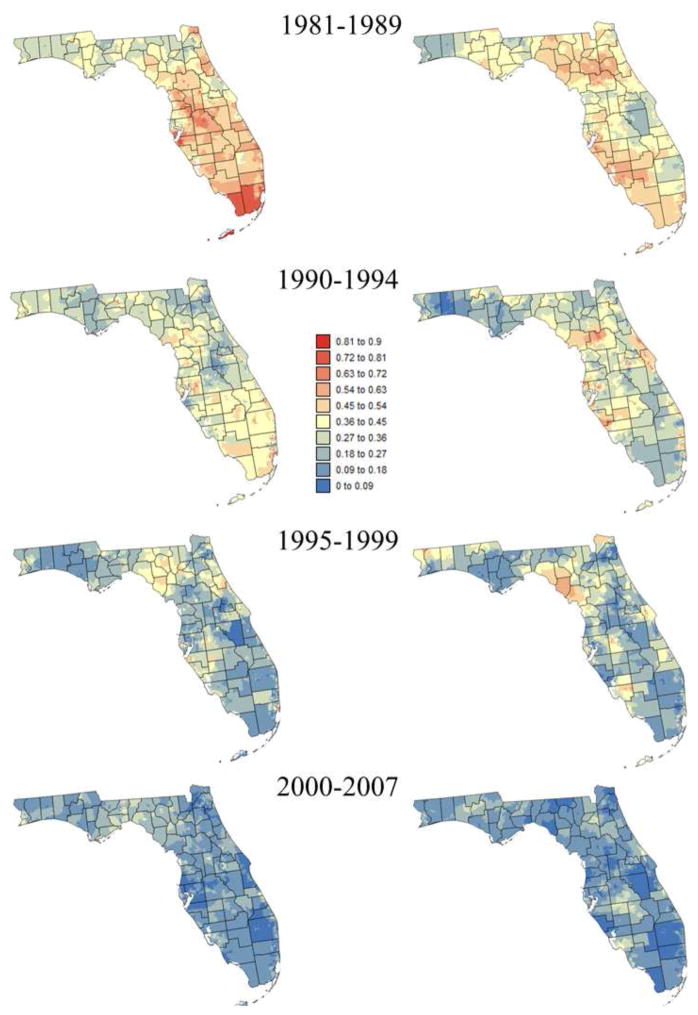
Smoothed census tracts proportions of late-stage diagnosis are mapped in Figures 3 and 4 for two race groups and two age categories: [40,64] and 65+. The series of maps clearly illustrate the statewide decline in proportion of late-stage diagnosis over time. It also highlights racial disparities (i.e. higher proportions of late-stage cases for black males) and the fact that late-stage diagnosis is more prevalent among younger patients (i.e. [40–64]), in particular prior to 1995 and for white males. Both races display distinct spatial patterns with higher rates of late-stage diagnosis in the Florida Panhandle for white males whereas high rates clustered in South-eastern Florida for black males.

Fig. 3.

Census-tract proportions of late-stage prostate cancer cases that were diagnosed for white males over four time periods and two age categories: [40–64] (left column) and [65,120] (right column). These rates were smoothed using binomial kriging.

Fig. 4.

Census-tract proportions of late-stage prostate cancer cases that were diagnosed for black males over four time periods and two age categories: [40–64] (left column) and [65,120] (right column). These rates were smoothed using binomial kriging.

A sensitivity analysis was conducted to investigate how the number of neighbors (i.e. census tracts) influences kriging results displayed in Figures 3 and 4. Kriging was performed repeatedly using a number of neighbors ranging from K=9 to 39 for white males, and K=12 to 48 for black males. In both cases, an increment of 3 neighbors was used. The impact on kriging results was quantified by the relative difference between rates estimated using K and (K+3) neighbors. As expected, increasing the number of neighbors has an incrementally smaller impact on kriging results (Figure 5). For black males the magnitude of relative changes increased initially when zero rate estimates were replaced by non-zero rates as more neighboring census tracts are used and late-stage cases are included. Figure 5 indicates that using K=18 for white males and K=36 for black males yields kriging estimates that are stable (i.e. rate of change < 3%, denoted by horizontal dashed line) without over-smoothing caused by larger search windows.

Fig. 5.

Time-averaged impact of the number K of neighbors on results of binomial kriging for both white and black males. The vertical axis represents the relative change in estimated rates when three more neighbors are included in kriging.

3.3 Analysis of temporal trends

A prerequisite to any finer analysis of temporal trends is the spatial aggregation of numbers of cases recorded annually within each census tract. Figure 1 first shows how the state wide proportion of late-stage diagnosis for white and black males changed with time according to the patient age. A joinpoint regression model was fitted and the hypothesis of parallelism of the two temporal trends was tested, which amounts at testing for the existence of racial disparities. Both age categories display opposite patterns. The rate of late-stage diagnosis for younger black males decreased through the entire time period whereas for white males the decline occurred only between 1998 and 2002 and at a slower pace, leading one to reject the hypothesis of parallelism (Fig. 1A). In addition, racial disparities within this age group got narrower over time to become negligible in the late 2000’s. On the contrary, proportions of late-stage diagnosis declined at similar pace for males 65+, resulting in no significant change in the relative magnitude of racial disparities and no rejection of the hypothesis of parallelism (Fig. 1B). A similar test of hypothesis was conducted to compare the temporal trends of the two age categories ([40,64] versus 65+) within each race group. Results in Table 3 (1^st line) indicate that unlike black males the trend models for white males are not parallel (null hypothesis is rejected): rates for younger white males declined at a slower pace than for the older generation, leading to a widening in disparities since the rates for 40–64 age group were larger to start with.

Table 3.

Results of tests of parallelism (R=reject, NR=non reject) for time series of proportions of late-stage diagnosis recorded for different races and age groups. Tests are conducted per class of increasing income (Class 1 to 5) and using a significance level α=0.05. The number ranging from 0 to 27 indicates the number of years where the 95% confidence intervals of APC for the two groups did not overlap.

	Black versus White		< 65 versus 65+
Income groups	< 65	65+	White	Black
All	R	NR	R	NR
Class 1	NR	NR	NR	NR
	6	3	8	1
Class 2	R	NR	NR	R
	13	7	3	23
Class 3	NR	NR	R	NR
	7	8	13	0
Class 4	NR	NR	R	NR
	8	27	5	0
Class 5	NR	NR	NR	NR
	2	15	3	9

Age groups: [40,64] (< 65) and 65 and older (65+)

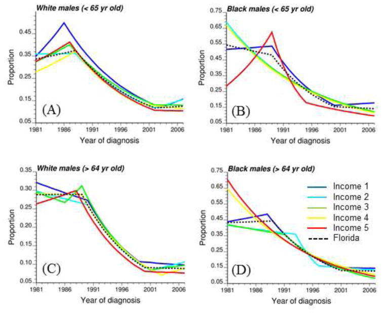
Figure 6 summarizes the impact of socio-economic status on temporal trends for the two age groups and two racial categories. For clarity, these graphs include only the joinpoint regression model fitted to each of the five classes of median household income as well as the statewide rates (i.e. all incomes combined, black dashed curve). Temporal trends among income classes are less similar for black males, in particular in 1980’s when rates of late-stage diagnosis can either sharply increase, either sharply decrease, or be relatively constant (Fig. 6B, D). These differences likely reflect the larger uncertainty of rates estimated from smaller minority populations, in particular younger black males (Table 1). The rate of decline is however generally faster for the highest incomes (classes 4 and 5). Temporal trends are much more similar for white males: for all five classes of income, proportion of late-stage diagnosis generally increased in the 1980’s for the 40–64 age group (Fig. 6A), while during the same time period it declined for cases over age 64 (Fig. 6C). In addition, rates observed in the most affluent census tracts (Income 5) were for most of the years lower than the rates recorded in the poorest neighborhoods (Income 1).

Fig. 6.

Joinpoint regression models fitted to time series of proportion of late-stage diagnosis computed for two age categories ([40–64], [65,120]), two race groups (white and black males), and five classes of increasing median household income (Income 1 → Income 5). The black dashed curve corresponds to the state wide trend model.

Comparing temporal trends for all age groups, racial categories and income classes would require plotting all 20 time series of Figure 6 on the same graph. Instead, multi-dimensional scaling was used to visualize similarities and differences between the 20 time series in a 2D space (N=2). The projection displayed in Figures 7 and 8 was based on the distance metrics described in Equations (7) and (8), respectively. Remember that time series close to each other in 2D share similar temporal trends; in other words, shorter distances correspond to smaller differences. The Shepard diagrams (not shown) indicate a better fit for the first distance metric (Equation 7) compared to Equation (8), although in both cases the observed dissimilarities are well reproduced by the MDS solution: rank correlation is 0.99 and 0.96, respectively. This is confirmed by the corresponding stress values, which are 0.04 and 0.18, indicating an excellent and fair goodness of fit according to Kruskal (1964). The fact that increasing the number of dimensions for the second criterion would only slightly reduce the stress value (e.g. 0.17 for N=4) indicates that N=2 is an acceptable solution.

Fig. 7.

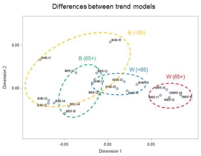
Results of multi-dimensional scaling applied to annual proportion of late-stage prostate cancer in Florida between 1981 and 2007. The 20 time series (2 races × 2 age groups × 5 income levels) were projected in a 2D space based on their dissimilarity quantified using an Euclidian distance metric: time series close to each other in 2D share similar temporal trends; the first letter denotes race (W,B), then age category (40–64, 65+), then income level (I1 – I5). Ellipses are drawn for visualization and have no statistical meaning.

Fig. 8.

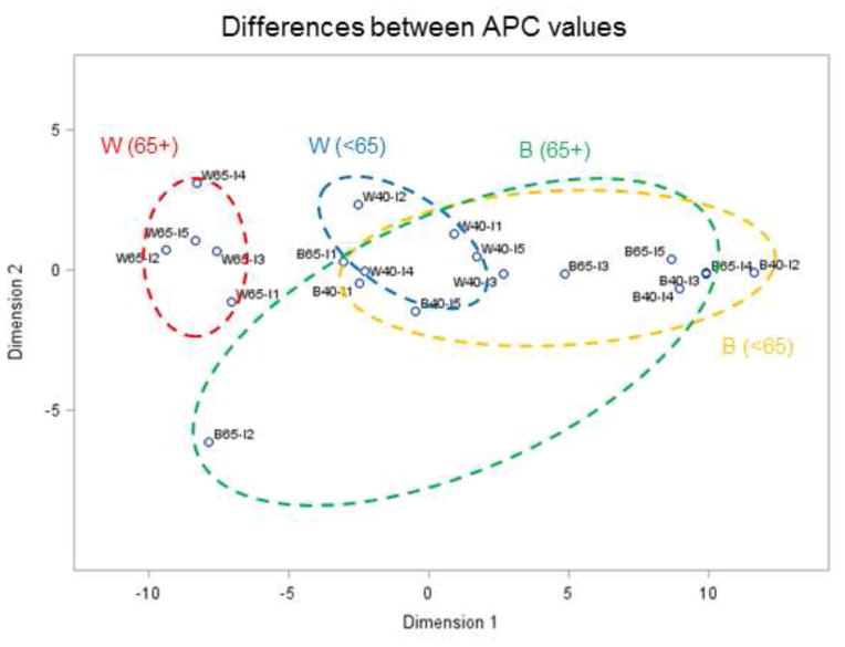
Results of multi-dimensional scaling applied to annual proportion of late-stage prostate cancer in Florida between 1981 and 2007. The 20 time series (2 races × 2 age groups × 5 income levels) were projected in a 2D space based on their dissimilarity quantified using an APC-based distance metric: time series close to each other in 2D share similar temporal trends; the first letter denotes race (W,B), then age category (40–64, 65+), then income level (I1 – I5). Ellipses are drawn for visualization and have no statistical meaning.

Regardless of the metric, MDS reveals tight clusters of time series for white males with clear separation of temporal trends according to the category of age. In both projections, older white males (65+) are clearly separate from the other age and race groups: ellipses, which were drawn manually for each group such as to encompass all five time series, do not overlap. The distinct behavior observed for older white males is explained by their overall lower percentage of late-stage diagnosis (Table 1) and their distinct temporal trend characterized by a steep decline between 1990 and 2000 which are preceded and followed by non-significant changes. Younger white males living in more affluent neighborhoods (W40-I4, W40-I5) have temporal trends closer to older white males (W65) who have lower rates of late-stage diagnosis in general (16.99%), see Figure 7.

Temporal trends are less similar for black males, which is illustrated by the larger spread of time series in the 2D space leading to bigger elliptical envelopes. This reflects the larger uncertainty of rates estimated from smaller populations. The spread of temporal trends for younger versus older black males differs depending on the distance metric used. The larger spread for younger males (< 65 yr) using metric #1 (Figure 7) reflects the greater magnitude of differences between trend models, in particular the highest income class (B40-I5) that is well separated from the others; see also Figure 6B. Metric # 2 captures differences in rate of changes instead of differences in proportions of late-stage diagnosis, resulting in larger spread for older black males (Figure 8).

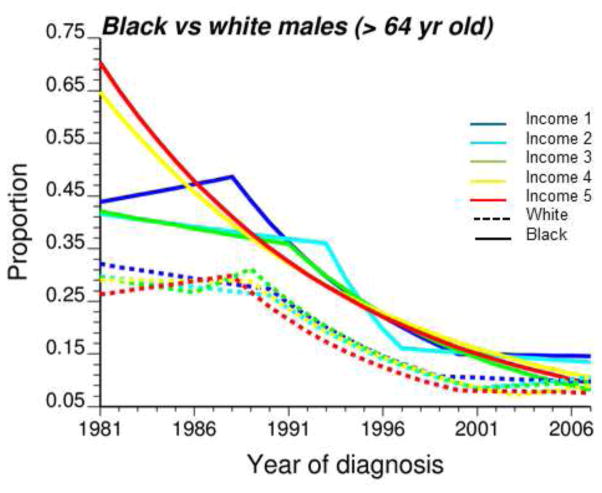
The visual comparison of temporal trends using MDS results was supplemented by a formal testing of the hypothesis of parallelism of trends conducted during the joinpoint regression analysis. Table 3 indicates that most of the time the null hypothesis of parallelism was not rejected. Because half of significant differences were found for comparison involving only white males (4^th column, income class 3 and 4), one can suspect a lack of power of other tests which were based on substantially smaller population sizes (Table 1). In that case, the disparity statistic B_cc′ (Equation 6) is more informative since it provides a metric ranging from 0 to 27 years of significant differences in APC instead of the binary result (i.e. Reject, Non Reject) of a global test of hypothesis. For example, although none of the tests conducted for males 65+ was significant, the statistic B_cc′ listed in Table 3 (3^rd column) indicates the presence of significant racial disparities in APC that lasted between 3 years (Income class 1) and 27 years (Income class 4). A closer look at the temporal trends for this age category highlights differences in temporal trends particularly for the two highest classes of incomes where no joinpoint was detected for black males while most of the decline for white males occurred between late 80’s and early 2000 (Figure 9). Medicare coverage could explain the similarity in temporal trends for white and black patients living in neighborhoods of lower socioeconomic status. On the other hand, better access to health care for the most affluent neighborhoods could explain the largest percentage of late-stage diagnosis recorded initially for black males.

Fig. 9.

Joinpoint regression models fitted to time series of proportion of late-stage diagnosis computed for white (dashed lines) and black males (solid lines) over age 64. Temporal trends were fitted for five classes of increasing median household income (Income 1 → Income 5).

4. Conclusions

The first contribution of this paper was to emphasize the distinct influence of age and socioeconomic status on proportions of prostate cancer late-stage diagnosis recorded for black and white males. On average over the entire study period, late-stage diagnosis was 20% more prevalent for black males 65+ compared to their younger counterpart, a trend opposite to what was observed for white males. The fact that the largest disparities between young and old black males were recorded in the most affluent neighborhoods suggests that PSA testing and further diagnostic evaluation are less frequent in the elderly, even in absence of financial obstacle to screening. The causes of disparities are multifactorial and complex. This study did not evaluate the role of patient perceptions of healthcare system/medical facilities, provider discussion of prostate cancer screening, or access to care. As such, this limits our interpretation of the current findings, and further research is needed. In addition to racial and socio-economic disparities in the magnitude of late-stage diagnosis frequency, joinpoint regression highlighted disparities in the temporal trends. The rate of decline in late-stage diagnosis for the two racial groups was similar among older patients (i.e. parallel time series), leading to no reduction in the relative magnitude of disparities. Conversely, for younger patients the decline occurred at a faster pace for black males with two important consequences: rates became similar to white males in the late 90s whereas the gap with black males 65+ was widening. The observed impact of socioeconomic and demographic factors on temporal trends in health outcomes emphasizes the need for local strategies and cancer control interventions to reduce prostate cancer late-stage diagnosis and improve health outcomes.

The other contribution of this paper was methodological. Although joinpoint regression is now routinely used to model temporal trends in health outcomes, fewer studies have applied the test of parallelism. The small sample size underlying tests conducted for extreme classes of median household income, in particular for minorities, explains the lack of power of tests which failed to detect any significant difference in parallelism for most of the pairs of temporal trends. The new disparity statistic allowed a finer analysis by computing the number of years the annual percent change of two temporal trends differs significantly. For example, the temporal trends modeled for white and black males 65+ residing in the census tracts with the two highest classes of incomes were not different enough to reject the hypothesis of parallelism, yet the disparity statistic indicated that annual percent changes were significantly different for most than half the time period (15 and 27 years).

Another novelty was the use of multi-dimensional scaling to visualize relationships among time series. MDS allows the projection of original data into a smaller space while preserving the original distance between time series. Two new metrics were introduced and they both led to a different representation of the overlap between age and racial groups based on whether the focus was on differences between mean trends or annual percent changes. This visual display can then be supplemented by a more detailed comparison of temporal trends for groups identified on the MDS 2D plot.

References

- Andriole GL, Crawford ED, Grubb RL, III, Buys SS, Chia D, Church TR, Reding DJ. Mortality results from a randomized prostate-cancer screening trial. New England Journal of Medicine. 2009;360(13):1310–1319. doi: 10.1056/NEJMoa0810696. [DOI] [PMC free article] [PubMed] [Google Scholar]
- Barratt AL, Stockler MR. Screening for prostate cancer: Explaining new trial results and their implications to patients. Med J Aust. 2009;191(4):226–229. doi: 10.5694/j.1326-5377.2009.tb02760.x. [DOI] [PubMed] [Google Scholar]
- Bechis SK, Carroll PR, Cooperberg MR. Impact of age at diagnosis on prostate cancer treatment and survival. Journal of Clinical Oncology: Official Journal of the American Society of Clinical Oncology. 2011;29(2):235–241. doi: 10.1200/JCO.2010.30.2075. [DOI] [PMC free article] [PubMed] [Google Scholar]
- Bernard J, Wilhelm N, Scherer M, May T, Schreck T. Time Series Paths: Projection-based explorative analysis of multivarate time series data. Journal of WSCG. 2012;20(2):97–106. [Google Scholar]
- BioMedware I. SpaceStat user manual version 4.1 2013 [Google Scholar]
- Brawn PN, Johnson EH, Kuhl DL, Riggs MW, Speights V, Johnson CF, Bell NF. Stage at presentation and survival of white and black patients with prostate carcinoma. Cancer. 1993;71(8):2569–2573. doi: 10.1002/1097-0142(19930415)71:8<2569::aid-cncr2820710822>3.0.co;2-r. [DOI] [PubMed] [Google Scholar]
- Carpenter WR, Howard DL, Taylor YJ, Ross LE, Wobker SE, Godley PA. Racial differences in PSA screening interval and stage at diagnosis. Cancer Causes & Control. 2010;21(7):1071–1080. doi: 10.1007/s10552-010-9535-4. [DOI] [PMC free article] [PubMed] [Google Scholar]
- Chu KC, Tarone RE, Freeman HP. Trends in prostate cancer mortality among black men and white men in the United States. Cancer. 2003;97(6):1507–1516. doi: 10.1002/cncr.11212. [DOI] [PubMed] [Google Scholar]
- Clegg LX, Reichman ME, Miller BA, Hankey BF, Singh GK, Lin YD, Chen VW. Impact of socioeconomic status on cancer incidence and stage at diagnosis: Selected findings from the surveillance, epidemiology, and end results: National longitudinal mortality study. Cancer Causes & Control. 2009;20(4):417–435. doi: 10.1007/s10552-008-9256-0. [DOI] [PMC free article] [PubMed] [Google Scholar]
- Do YK, Carpenter WR, Spain P, Clark JA, Hamilton RJ, Galanko JA, Godley PA. Race, healthcare access and physician trust among prostate cancer patients. Cancer Causes & Control. 2010;21(1):31–40. doi: 10.1007/s10552-009-9431-y. [DOI] [PMC free article] [PubMed] [Google Scholar]
- Goovaerts P. Kriging and semivariogram deconvolution in the presence of irregular geographical units. Mathematical Geosciences. 2008;40(1):101–128. [PMC free article] [PubMed] [Google Scholar]
- Goovaerts P. Combining area-based and individual-level data in the geostatistical mapping of late-stage cancer incidence. Spatial and Spatio-Temporal Epidemiology. 2009;1(1):61–71. doi: 10.1016/j.sste.2009.07.001. [DOI] [PMC free article] [PubMed] [Google Scholar]
- Goovaerts P, Xiao H. Geographical, temporal and racial disparities in late-stage prostate cancer incidence across Florida: A multiscale joinpoint regression analysis. International Journal of Health Geographics. 2011;10(1):63. doi: 10.1186/1476-072X-10-63. [DOI] [PMC free article] [PubMed] [Google Scholar]
- Hayanga AJ, Kaiser HE, Sinha R, Berenholtz SM, Makary M, Chang D. Residential segregation and access to surgical care by minority populations in US counties. Journal of the American College of Surgeons. 2009;208(6):1017–1022. doi: 10.1016/j.jamcollsurg.2009.01.047. [DOI] [PubMed] [Google Scholar]
- Henry KA, Boscoe FP. Estimating the accuracy of geographical imputation. International Journal of Health Geographics. 2008;7(1):3. doi: 10.1186/1476-072X-7-3. [DOI] [PMC free article] [PubMed] [Google Scholar]
- Hoffman RM, Gilliland FD, Eley JW, Harlan LC, Stephenson RA, Stanford JL, Potosky AL. Racial and ethnic differences in advanced-stage prostate cancer: The prostate cancer outcomes study. Journal of the National Cancer Institute. 2001;93(5):388–395. doi: 10.1093/jnci/93.5.388. [DOI] [PubMed] [Google Scholar]
- Jones BA, Liu WL, Araujo AB, Kasl SV, Silvera SN, Soler-Vila H, Dubrow R. Explaining the race difference in prostate cancer stage at diagnosis. Cancer Epidemiology, Biomarkers & Prevention: A Publication of the American Association for Cancer Research, Cosponsored by the American Society of Preventive Oncology. 2008;17(10):2825–2834. doi: 10.1158/1055-9965.EPI-08-0203. [DOI] [PubMed] [Google Scholar]
- Kim H, Fay MP, Feuer EJ, Midthune DN. Permutation tests for joinpoint regression with applications to cancer rates. Statistics in Medicine. 2000;19(3):335–351. doi: 10.1002/(sici)1097-0258(20000215)19:3<335::aid-sim336>3.0.co;2-z. [DOI] [PubMed] [Google Scholar]
- Kim H, Fay MP, Yu B, Barrett MJ, Feuer EJ. Comparability of segmented line regression models. Biometrics. 2004;60(4):1005–1014. doi: 10.1111/j.0006-341X.2004.00256.x. [DOI] [PubMed] [Google Scholar]
- Kim HJ, Yu B, Feuer EJ. Selecting the number of change-points in segmented line regression. Statistica Sinica. 2009;19(2):597–609. [PMC free article] [PubMed] [Google Scholar]
- Kruskal JB. Multidimensional scaling by optimizing goodness of fit to a nonmetric hypothesis. Psychometrika. 1964;29:1–27. [Google Scholar]
- Laiyemo AO, Doubeni C, Pinsky PF, Doria-Rose VP, Bresalier R, Lamerato LE, Berg CD. Race and colorectal cancer disparities: health-care utilization vs different cancer susceptibilities. Journal of the National Cancer Institute. 2010;102(8):538–546. doi: 10.1093/jnci/djq068. [DOI] [PMC free article] [PubMed] [Google Scholar]
- Lerman P. Fitting segmented regression models by grid search. Applied Statistics. 1980;29(1):77–84. [Google Scholar]
- Lillo-Castellano J, Mora-Jiménez I, Santiago-Mozos R, Rojo-Álvarez J, Ramiro-Bargueño J, Algora-Weber A. Weaning outcome prediction from heterogeneous time series using normalized compression distance and multidimensional scaling. Expert Systems with Applications. 2013;40(5):1737–1747. [Google Scholar]
- Morton RA., Jr Racial differences in adenocarcinoma of the prostate in North American men. Urology. 1994;44(5):637–645. doi: 10.1016/s0090-4295(94)80196-7. [DOI] [PubMed] [Google Scholar]
- Musa D, Schulz R, Harris R, Silverman M, Thomas SB. Trust in the health care system and the use of preventive health services by older black and white adults. American Journal of Public Health. 2009;99(7):1293–1299. doi: 10.2105/AJPH.2007.123927. [DOI] [PMC free article] [PubMed] [Google Scholar]
- Robbins AS, Whittemore AS, Thom DH. Differences in socioeconomic status and survival among white and black men with prostate cancer. American Journal of Epidemiology. 2000;151(4):409–416. doi: 10.1093/oxfordjournals.aje.a010221. [DOI] [PubMed] [Google Scholar]
- Salinas CA, Tsodikov A, Ishak-Howard M, Cooney KA. Prostate cancer in young men: An important clinical entity. Nature Reviews Urology. 2014;11(6):317–323. doi: 10.1038/nrurol.2014.91. [DOI] [PMC free article] [PubMed] [Google Scholar]
- SAS Institute Inc. SAS/STAT 9.3 User’s guide. Cary, NC: SAS Institute Inc; 2011. [Google Scholar]
- Schröder FH, Hugosson J, Roobol MJ, Tammela TL, Ciatto S, Nelen V, Zappa M. Screening and prostate-cancer mortality in a randomized European study. New England Journal of Medicine. 2009;360(13):1320–1328. doi: 10.1056/NEJMoa0810084. [DOI] [PubMed] [Google Scholar]
- Schwartz KL, Crossley-May H, Vigneau FD, Brown K, Banerjee M. Race, socioeconomic status and stage at diagnosis for five common malignancies. Cancer Causes & Control. 2003;14(8):761–766. doi: 10.1023/a:1026321923883. [DOI] [PubMed] [Google Scholar]
- Scosyrev E, Messing EM, Mohile S, Golijanin D, Wu G. Prostate cancer in the elderly. Cancer. 2012;118(12):3062–3070. doi: 10.1002/cncr.26392. [DOI] [PubMed] [Google Scholar]
- Sheehan TJ, DeChello LM, Kulldorff M, Gregorio DI, Gershman S, Mroszczyk M. The geographic distribution of breast cancer incidence in massachusetts 1988 to 1997, adjusted for covariates. International Journal of Health Geographics. 2004;3(1):17. doi: 10.1186/1476-072X-3-17. [DOI] [PMC free article] [PubMed] [Google Scholar]
- Shepard R. Representation of structure in similarity data: Problems and prospects. Psychometrika. 1974;39:373–421. [Google Scholar]
- Smart CR. The results of prostate carcinoma screening in the US as reflected in the surveillance, epidemiology, and end results program. Cancer. 1997;80(9):1835–1844. doi: 10.1002/(sici)1097-0142(19971101)80:9<1835::aid-cncr23>3.0.co;2-5. [DOI] [PubMed] [Google Scholar]
- Virnig BA, Baxter NN, Habermann EB, Feldman RD, Bradley CJ. A matter of race: Early-versus late-stage cancer diagnosis. Health Affairs (Project Hope) 2009;28(1):160–168. doi: 10.1377/hlthaff.28.1.160. [DOI] [PMC free article] [PubMed] [Google Scholar]
- Wachtel MS, Nelius T, Haynes AL, Dahlbeck S, de Riese W. PSA screening and deaths from prostate cancer after diagnosis--a population based analysis. Prostate. 2013;73:1365–1369. doi: 10.1002/pros.22680. [DOI] [PubMed] [Google Scholar]
- Ward EM, Fedewa SA, Cokkinides V, Virgo K. The association of insurance and stage at diagnosis among patients aged 55 to 74 years in the national cancer database. The Cancer Journal. 2010;16(6):614–21. doi: 10.1097/PPO.0b013e3181ff2aec. [DOI] [PubMed] [Google Scholar]
- Webster R, Oliver M, Muir K, Mann J. Kriging the local risk of a rare disease from a register of diagnoses. Geographical Analysis. 1994;26(2):168–185. [Google Scholar]
- Wolf A, Wender RC, Etzioni RB, Thompson IM, D’Amico AV, Volk RJ, Andrews K. American cancer society guideline for the early detection of prostate cancer: Update 2010. CA: A Cancer Journal for Clinicians. 2010;60(2):70–98. doi: 10.3322/caac.20066. [DOI] [PubMed] [Google Scholar]
- Xiao H, Tan F, Goovaerts P, Adunlin G, Ali A, Huang Y, Gwede CK. Factors associated with time-to-treatment of prostate cancer in Florida. Journal of Health Care for the Poor and Underserved. 2014;24(4):132–146. doi: 10.1353/hpu.2014.0005. [DOI] [PMC free article] [PubMed] [Google Scholar]