

Abstract
Behavioral momentum theory suggests that the relation between a discriminative-stimulus situation and reinforcers obtained in that context (i.e., the Pavlovian stimulus–reinforcer relation) governs persistence of operant behavior. Within the theory, a mass-like aspect of behavior has been shown to be a power function of predisruption reinforcement rates. Previous investigations of resistance to change in multiple schedules, however, have been restricted to examining response persistence following protracted periods of stability in reinforcer rates within a discriminative situation. Thus, it is unclear how long a stimulus–reinforcer relation must be in effect prior to disruption in order to affect resistance to change. The present experiment examined resistance to change of pigeon’s key pecking following baseline conditions where reinforcer rates that were correlated with discriminative-stimulus situations changed. Across conditions, one multiple-schedule component arranged either relatively higher rates or lower rates of variable-interval food delivery, while the other component arranged the opposite rate. These schedules alternated between multiple-schedule components across blocks of sessions such that reinforcer rates in the components were held constant for 20, 5, 3, 2, or 1 session(s) between alternations. Resistance to extinction was higher in the component that most recently was associated with higher rates of food delivery in all conditions except when schedules alternated daily or every other day. These data suggest that resistance to change in multiple schedules is related to recently experienced reinforcer rates but only when multiple-schedule components are associated with specific reinforcer rates for several sessions.
Keywords: resistance to change, behavioral momentum, changing reinforcer rates, extinction, key pecking, pigeons
Persistence of discriminated operant behavior tends to be positively related to baseline reinforcer rates. For example, Nevin (1974) trained pigeons to peck keys for food in two-component multiple schedules, where two stimulus situations, signaled by different key-light colors, alternated successively within sessions. In the presence of one key-light color, pecking produced food relatively frequently according to a variable-interval (VI) schedule, and in the presence of the other color, VI food was delivered relatively infrequently. When responding subsequently was challenged by presenting free food during intercomponent intervals (ICIs) or by extinction, responding in the component associated with high-rate reinforcement was more resistant to change than responding in the component associated with low-rate reinforcement. This finding is general to the study of resistance to change in multiple schedules and has been demonstrated in several species (e.g., humans, rats, and goldfish; Blackman, 1968; Cohen, 1996; Grimes & Shull, 2001; Igaki & Sakagami, 2004; Mace et al., 1990; Shahan & Burke, 2004) using a variety of different disruptors (e.g., presession feeding, aversive consequences, and distraction; see Craig, Nevin, & Odum, 2014; Nevin, 1992; 2002; Nevin & Grace, 2000, for review). Note, though, that some limited evidence suggests that factors other than frequency of baseline reinforcer delivery can influence resistance to change (see, e.g., Bell, 1999; Lattal, 1989; Nevin, Grace, Holland, & McLean, 2001; Podlesnik, Jimenez-Gomez, Ward, & Shahan, 2006).
Behavioral momentum theory (Nevin, Mandel, & Atak, 1983) offers a conceptual and quantitative framework that may be used to describe the contribution of reinforcer deliveries to resistance to change. According to momentum theory, response persistence in the face of disruption is a function of a mass-like quality of behavior engendered by reinforcer deliveries in a given stimulus situation (e.g., a multiple-schedule component). As reinforcer rates in a stimulus situation increase, the Pavlovian stimulus–reinforcer relation in the situation is strengthened, thereby producing greater behavioral mass and resistance to change (for discussion, see Nevin, 1992; 2002; Nevin, Tota, Torquato, & Shull, 1990).
Quantitatively, the positive relation between resistance to change and baseline reinforcer rates may be expressed as follows (see Nevin, Mandel, & Atak, 1983; Nevin & Shahan, 2011):
| (1) |
The left side of Equation 1 is log-transformed proportion-of-baseline response rates given a disruptor. The right side of the equation represents those factors that contribute to responding during disruption and may be broken into two more general terms. The numerator represents the negative impact of the disruptor on responding, where x varies with the magnitude of the disruptor applied (e.g., the amount of food given to a hungry animal during presession feeding preparations in the animal laboratory). The denominator of Equation 1 is thought to correspond to a mass-like construct that governs the persistence of behavior and has been shown to be a power function of predisruption reinforcer rates (Nevin, 1992). Thus, r is baseline reinforcer rates, in reinforcers delivered per hr, and b is a free parameter that represents sensitivity to baseline reinforcer rates. The b parameter typically assumes a value near 0.5 when Equation 1 is fitted to disruption data from multiple schedules (see Nevin, 2002).
The numerator of Equation 1 may be expanded as follows to account for the specific effects of extinction as a disruptor:
| (2) |
Here, t is time in extinction, measured in sessions, and c is the impact on responding of suspending the response–reinforcer contingency (a free parameter typically assuming a value near 1; Nevin & Grace, 2000). The parameters d and Δr collectively represent the impact on responding of transitioning from a period of reinforcement during baseline to a period of nonreinforcement during extinction (i.e., generalization decrement) where Δr is the change in reinforcer rates between baseline and extinction (in reinforcers omitted per hr) and d is a scaling parameter that is free to vary and typically assumes a value near 0.001.
The quantitative theory of resistance to change offered by Equations 1 and 2 accounts for an array of persistence data obtained from multiple-schedule preparations (for review, see Nevin, 1992; 2002; 2012; Nevin & Shahan, 2011). When these models are used to describe resistance to change from these situations, behavioral mass typically is characterized by setting r in the denominator equal to programmed predisruption reinforcer rates. In addition, all investigations of resistance to change have examined response persistence following prolonged exposure to stable baseline reinforcer rates. Under these conditions, the method by which one calculates reinforcer rates (i.e., r) essentially is inconsequential: Under VI schedules, which conventionally are used in resistance-to-change research, mean obtained reinforcer rates in a multiple-schedule component over any number of sessions should approximate programmed reinforcer rates in that component. It is unclear, then, if resistance to change depends on longer-term reinforcer rates (i.e., mean reinforcer rate for a given component over the entirety of baseline) or on reinforcer rates from some smaller subset of recently experienced sessions (e.g., the mean reinforcer rate for a given component from the two most recent sessions preceding disruption). In short, it is unknown how long particular discriminative stimulus–reinforcer situations must be in effect before the reinforcer rates signaled by those stimuli affect the persistence of responding.
Thus, the purpose of the present experiment was to determine if the temporal epoch over which discriminative stimulus–reinforcer relations are in effect prior to disruption impacts relative resistance to that disruption. To this end, pigeons pecked keys in multiple schedules of reinforcement in which the component stimuli signaled different reinforcement rates for a larger or smaller number of sessions prior to disruption. Overall baseline reinforcer rates in the multiple-schedule components were the same when calculated across conditions but differed between components immediately before extinction testing. The number of sessions during which these differences were held constant prior to extinction was varied between conditions.
Method
Subjects
Seven unsexed homing pigeons with previous experience responding under schedules of positive reinforcement served in all conditions of the experiment. An eighth unsexed homing pigeon, also with experience responding under schedules of positive reinforcement, was included in conditions 3 through 7. Pigeons were housed separately in a temperature-controlled colony room with a 12:12 hr light/dark cycle and were maintained at 80% of their free-feeding weights by the use of supplementary postsession feedings as necessary. Each pigeon had free access to water when not in sessions. Animal care and all procedures detailed below were conducted in accordance with guidelines set forth by Utah State University’s Institutional Animal Care and Use Committee.
Apparatus
Four Lehigh Valley Electronics operant chambers for pigeons (dimensions 35 cm long, 35 cm high, and 30 cm wide) were used. Each chamber was constructed of painted aluminum and had a brushed-aluminum work panel on the front wall. Each work panel was equipped with three equally spaced response keys. Only the center key was used in this experiment and was transilluminated various colors to signal the different components of the multiple schedule across pigeons and conditions (see the Appendix for a list of stimulus assignments). A force of at least 0.1 N was required to operate the key. A rectangular food aperture (5 cm wide by 5.5 cm tall, with its center 10 cm above the floor of the chamber) also was located on the work panel. The food aperture was illuminated by a 28-v DC bulb during reinforcer deliveries, which consisted of 1.5 s of access to Purina Pigeon Checkers collected from a hopper in the illuminated aperture. This reinforcer duration is standard for our laboratory and ensures maintenance of pigeons’ criterion weights given that pigeon chow is a denser food source by volume than mixed grain. General illumination was provided at all times by a 28-v DC house light that was centered 4.5 cm above the center response key, except during blackout periods and reinforcer deliveries. A ventilation fan and a white-noise generator masked extraneous sounds at all times. Timing and recording of experimental events was controlled by Med PC software that was run on a PC computer in an adjoining control room.
Procedure
Under all conditions of the experiment, pigeons key-pecked for food under a two-component multiple schedule with the following specifications: Each component of the multiple schedule lasted for 3 min, components were separated by 30-s ICIs, and each session consisted of 10 strictly alternating components (i.e., 30 min of session time, excluding time for ICIs and reinforcer deliveries). The first component that occurred was randomly determined at the start of each session.
One multiple-schedule component stimulus initially signaled a VI 30-s schedule of reinforcement (i.e., the rich schedule) while the other component stimulus initially signaled a VI 120-s schedule of reinforcement (i.e., the lean schedule). Both VI schedules consisted of 10 intervals derived from Fleshler and Hoffman’s (1962) constant-probability algorithm. In each condition, the component stimuli associated with rich and lean reinforcement schedules were constant within sessions but alternated across sessions for the entirety of baseline. The number of sessions between each alternation was 20, 5, 3, 2, or 1 session(s), depending on the condition. For example, in the 5-Day alternation condition, one component stimulus signaled the rich schedule while the other component stimulus signaled the lean schedule for five sessions. Then, schedule–stimulus associations changed such that the component that first signaled the rich schedule signaled the lean schedule, and the component that first signaled the lean schedule signaled the rich schedule, for another five sessions. Alternations of the component stimuli associated with rich and lean schedules continued across blocks of sessions specified by each condition until baseline ended. In each condition, schedule alternations were arranged such that the component that started rich ended lean (hereafter the “Rich-to-Lean” component) and the schedule that started lean ended rich (hereafter the “Lean-to-Rich” component) prior to extinction testing. Consequently, both multiple-schedule component stimuli were associated with the VI 30-s and VI 120-s schedules for an equal number of sessions, and overall rates of reinforcement were the same for each component when averaged over the entirety of baseline. Further, the VI 120-s schedule was in effect in the Rich-to-Lean component, and the VI 30-s schedule was in effect in the Lean-to-Rich component, just prior to extinction testing. The chronological list of conditions (including the number of sessions per schedule alternation and the number of sessions per condition) can be found in Table 1.
Table 1.
Condition Order, Number of Sessions per Baseline Condition, and Component-Wide food Rates
| Condition | Sessions | Component-Wide Foods/Min Mean (SEM) |
|
|---|---|---|---|
| Lean-Rich | Rich-Lean | ||
| 20-Day | 40 | 1.14 (0.04) | 1.15 (0.04) |
| 1-Day | 30 | 1.15 (0.05) | 1.14 (0.05) |
| 5-Day | 30 | 1.15 (0.05) | 1.14 (0.05) |
| 3-Day | 30 | 1.15 (0.05) | 1.15 (0.05) |
| 2-Day | 32 | 1.15 (0.05) | 1.15 (0.05) |
| 5-Day (Rep.) | 30 | 1.14 (0.05) | 1.14 (0.05) |
| 20-Day (Rep.) | 40 | 1.14 (0.04) | 1.16 (0.05) |
Following each baseline schedule, extinction was assessed for five sessions. In extinction, the stimulus situation was the same as during the preceding baseline condition. Responding, however, had no consequences.
Results
Mean obtained reinforcer rates for both components across sessions of baseline in each condition are shown in Figure 1. Obtained reinforcer rates within a component approximated programmed reinforcer rates. Importantly, there were no noticeable decreases in overall obtained reinforcer rates following a change in schedule value. That is, obtained reinforcer rates between components were maintained across the course of a condition. Mean (plus standard error of the mean; SEM) overall, component-wide reinforcer rates for each condition are included in Table 1. These rates were virtually the same across components and conditions.
Fig. 1.

Mean reinforcer per min (plus SEM) from both multiple-schedule components across sessions of each baseline condition.
Mean response rates across sessions of baseline in both components for each condition are shown in Figure 2. Response rates tended to track reinforcer rates across baseline sessions. That is, response rates tended to be higher in the component that was associated with the VI 30-s schedule of reinforcement during a session, and lower in the component that was associated with the VI 120-s schedule. A change in reinforcer rate for a given component was accompanied by a change in response rate for that component, usually within the first session following the change in reinforcer rate. For example, the Rich-to-Lean component in the 20-Day alternation conditions arranged VI 30-s food for the first 20 sessions of baseline, after which this component arranged VI 120-s food for the remaining 20 sessions (see top panels of Fig. 1). Response rates in this component were higher than in the Lean-to-Rich component for the first 20 sessions of baseline (when that component signaled the VI 30-s schedule) but were lower than in the Lean-to-Rich component for the last 20 sessions of baseline (when that component signaled the VI 120-s schedule). A similar patterning of changes in response rate following changes in reinforcer rate was present in each of the other conditions.
Fig. 2.

Mean responses per min (plus SEM) from both multiple-schedule components across sessions of each baseline condition.
The extent to which differences in resistance to extinction between components were associated with frequency of baseline-schedule alternation was examined using relative resistance-to-extinction measures (see Grace & Nevin, 1997). First, proportion-of-baseline response rates were calculated for each subject in each condition by dividing response rates during each session of extinction by response rates during the last session of the corresponding baseline condition.1 Then, relative resistance to extinction was calculated by averaging proportion-of-baseline response rates across all five sessions of extinction separately for each component and in each condition. This value for the Lean-to-Rich component in a condition then was divided by the equivalent measure for the Rich-to-Lean component, after which this ratio was log transformed. Values of 0 indicate no difference in resistance to extinction between Lean-to-Rich and Rich-to-Lean components, values greater than 0 indicate greater resistance to extinction in the Lean-to-Rich component, and values less than 0 indicate greater resistance to extinction in the Rich-to-Lean component. Results of this analysis for each condition of the experiment are shown in Figure 3. Bars represent mean relative-resistance measures, and individual data points represent these measures for individual subjects. Data are plotted with respect to frequency of schedule alternation within a condition and not order of condition presentation.
Fig. 3.

Relative-resistance-to-extinction (Lean-to-Rich/Rich-to-Lean; see text for details) measures aggregated across subjects for each condition. Bars represent group means and data points represent measures for individual subjects. From left to right, data are shown from the 20-Day, 5-Day, 3-Day, 2-Day, 1-Day, 20-Day-Replication, and 5-Day replication conditions.
Without exception, resistance to extinction was greater in the Lean-to-Rich component (i.e., the component that arranged VI 30-s food in the sessions just before extinction testing) than in the Rich-to-Lean component (i.e., the component that arranged VI 120-s food in the sessions just before extinction testing) in the 20-Day, 5-Day, and 3-Day alternation conditions. There were not, however, systematic differences in relative resistance to extinction between these conditions. In the 2-Day and 1-Day alternation conditions, resistance to extinction was not systematically higher in one component than in the other component. Relative resistance to extinction from replication of the 20-Day alternation condition was essentially the same as the first 20-Day alternation condition. Though resistance to extinction tended to be higher in the Lean-to-Rich component than in the Rich-to-Lean component during replication of the 5-Day alternation condition, the effect was not as pronounced as it was during the initial 5-Day alternation condition. A one-way repeated-measures ANOVA was conducted on relative resistance-to-extinction measures to further examine mean differences in these measures between conditions. The main effect was significant, F(6, 36) = 10.67, p < .001. Least-significant difference post-hoc comparisons were conducted to examine this main effect more closely. These comparisons used estimated marginal mean scores for relative resistance to extinction from each condition to determine for which conditions relative resistance to extinction differed. Results from this analysis are summarized in Table 2. Most importantly, these post-hoc analyses revealed that relative resistance to extinction differed significantly between those conditions in which responding was more persistent in the Lean-to-Rich component than in the Rich-to-Lean component (i.e., the 20-Day, 5-Day, and 3-Day alternation conditions) and those conditions in which no differential resistance to extinction was observed (i.e., the 2-Day and 1-Day alternation conditions).
Table 2.
Absolute Mean Differences between Grouped Relative-Resistance-to-Extinction Measures from Each Condition
| Condition/Condition | 20-Day | 20-Day (Rep.) | 5-Day | 5-Day (Rep.) | 3-Day | 2-Day | 1-Day |
|---|---|---|---|---|---|---|---|
| 20-Day | - | - | - | - | - | - | - |
| 20-Day (Rep.) | −0.033 (.058) | - | - | - | - | - | - |
| 5-Day | −0./057 (.078) | −0.024 (.084) | - | - | - | - | - |
| 5-Day (Rep. | 0.212* (.079) | 0.245* (.088) | 0.207* (.082) | - | - | - | - |
| 3-Day | 0.116 (.077) | 0.149 (.069) | 0.173 (.101) | −0.097 (.052) | - | - | - |
| 2-Day | 0.370* (.080) | 0.403* (.067) | 0.427* (.082) | 0.158 (.068) | 0.254* (.072) | - | - |
| 1-Day | 0.309* (.050) | 0.342* (.059) | 0.366* (.094) | 0.097 (.075) | 0.193* (.057) | −0.061 (.054) | - |
Mean difference is statistically significant (p < .05)
Note: Values in parentheses represent SEM.
Relative resistance to extinction provides a measure of differences in resistance to extinction between components, but this measure is limited in that it does not necessarily show the origins of these differences. For example, a relative resistance-to-extinction value of 0 could indicate that proportion-of-baseline response rates in both multiple-schedule components were virtually unaffected by extinction or that responding occurred at zero rates in both multiple-schedule components across sessions of extinction. Accordingly, comparisons of proportion-of-baseline response rates between conditions were conducted to determine if the frequency of schedule alternation during baseline affected rate of extinction. Proportion-of-baseline response rates (calculated here as above) across extinction sessions for each condition (excluding 5-Day and 20-Day replications for clarity of display), separated for each component, are shown in Figure 4. Data from the Rich-to-Lean component are shown in the top panel of this figure, and data from the Lean-to-Rich component are shown in the bottom panel.
Fig. 4.

Mean (plus SEM) proportion-of-baseline response rates across sessions of extinction for the Rich-to-Lean (top panel) and Lean-to-Rich (bottom panel) components.
Proportion-of-baseline response rates in the 2-Day and 1-Day alternation conditions in the Rich-to-Lean component were elevated above those rates from the remaining components during the second and third sessions of extinction testing. A 7 X 6 (Condition X Session) repeated-measure ANOVA conducted on these data revealed significant main effects of Condition, F(6, 36) = 2.48, p < .05, and Session, F(5, 30) = 139.94, p < .001, but a nonsignificant interaction between these terms, F(30, 180) = 1.30, NS. Least-significant-difference post-hoc tests based on estimated marginal means for Condition revealed that extinction progressed significantly faster in the 5-Day and replication of the 20-Day alternation conditions than in the 2-Day alternation condition. In the Lean-to-Rich component, responding was less resistant to extinction in the 2-Day and 1-Day alternation conditions during the first session of extinction, but the extinction functions did not differ systematically thereafter. A 7 X 6 (Condition X Session) repeated-measures ANOVA conducted on these data revealed a significant main effect of Session and a significant Condition X Session interaction (respectively, F[5, 30] = 78.61, p < .001; and F[30, 180] = 1.70, p < .05). The main effect of Condition was nonsignificant, F(2.69, 16.14) = 2.14, NS (note that Greenhouse-Geisser corrections for degrees of freedom were used because, according to Mauchly’s method, the assumption of sphericity for Condition was violated). Thus, differences in resistance to extinction between conditions depended on session, as suggested above. In summary, resistance to extinction was lower in the 2-Day and 1-Day alternation conditions than in the other conditions during the first day of extinction in the Lean-to-Rich component. Further, in the Rich-to-Lean component, responding tended to persist to a greater degree in the 2-Day and 1-Day alternation conditions than in the other conditions. This difference was only statistically significant, however, between the 2-Day alternation condition and the 5-Day and replication of the 20-Day alternation conditions.
To examine how frequency of baseline-schedule alternation affected estimates of behavioral mass, Equation 2 was fitted to mean log proportion-of-baseline response rates several different ways via least-squares regression using Microsoft Excel Solver. Data from replication of the 20-Day and 5-Day conditions were excluded from these analyses. There is no principled reason to believe that alternation of stimulus–reinforcer relations during baseline should change the disruptive impacts of suspending the response–reinforcer contingency or of generalization decrement during extinction. Accordingly, for all fits, the free parameters c and d were fixed at 1 and 0.001, respectively, and the Δr term in the numerator was fixed to 30 and 120 reinforcers omitted per hr for the Rich-to-Lean and Lean-to-Rich components, respectively.
First, to determine how behavioral mass, per se, was impacted by frequency of schedule alternation, the denominator of the equation was collapsed into a composite mass term that was free to vary between components. This mass composite was substantially larger in the Lean-to-Rich component than in the Rich-to-Lean component in the 20-Day, 5-Day, and 3-Day alternation conditions but similar between components in the 2-Day and 1-Day alternation conditions (see the top-left panel of Fig. 5). Next, to determine if these changes in mass could be attributed to changes in sensitivity to baseline reinforcer rates, the r parameter in the denominator of the model was fixed at 30 and 120 reinforcers per hr for the Rich-to-Lean and Lean-to-Rich components, respectively, while b was free to vary. Sensitivity to baseline reinforcer rates did not change systematically between conditions (see the top-right panel of Fig. 5). Thus, changes in b likely did not produce the observed changes in relative resistance to extinction across conditions. Finally, b was allowed to vary as in the previous fit, and the reinforcer-rate terms in the denominator (i.e., r) were allowed to vary between components as a parameter. In this fit, b assumed similar values as in the previous fit (see the bottom-right panel of Fig. 5), but the reinforcer-rate terms (r in the bottom-left panel of Fig. 5) were substantially larger in the Lean-to-Rich component than in the Rich-to-Lean component in the 20-Day, 5-Day, and 3-Day alternation conditions. These parameter values were similar between components in the 2-Day and 1-Day alternation conditions.
Fig. 5.
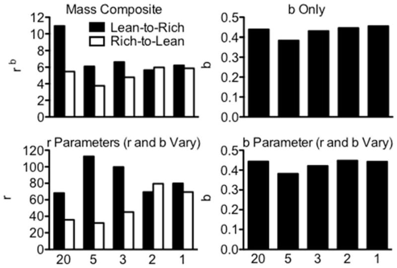
Parameter values from fits of the augmented model of resistance to extinction data obtained from each condition. Top left: composite-mass values (rb). Top right: sensitivity values (b) when only this parameter was allowed to vary. Bottom left: baseline-reinforcer-rate values (r in the denominator of Eq. 2) from both components when b was allowed to vary and shared by both components and r was allowed to vary between components. Bottom right: sensitivity values when b was allowed to vary and shared by both components and r was allowed to vary between components. From left to right, data are shown from the 20-Day, 5-Day, 3-Day, 2-Day, and 1-Day alternation conditions.
Discussion
Behavioral momentum theory is centrally concerned with the relation between Pavlovian stimulus–reinforcer contingencies and persistence of discriminated, free-operant responding (see Craig, Nevin, & Odum, 2014; Nevin, 2012; Nevin & Grace, 2000). Despite the well-established Pavlovian determination of resistance to change (e.g., Nevin, 1984; Nevin, Tota, Torquato, & Shull, 1990), no research previously has examined the timeframe over which stimulus–reinforcer relations have functional effects on resistance to change in multiple schedules. Investigations of resistance to change historically have focused on response persistence following periods of prolonged exposure to stable baseline reinforcer rates, precluding identification of how behavioral mass (i.e., the term in the denominators of Eqs. 1 and 2) accumulates in these conditioning situations.
The present experiment aimed to address this gap in the literature by arranging situations in which stimulus–reinforcer relations varied over the course of baseline. If, for example, resistance to change depended on the association between condition-wide reinforcer rates (i.e., the average reinforcer rate in a given stimulus situation across baseline) and multiple-schedule component stimuli, proportion-of-baseline response rates across sessions of extinction should have been the same in both multiple-schedule components in all conditions because both stimulus situations were correlated with VI 30-s and VI 120-s food for an equal number of sessions. If resistance to change depended only on the association between stimuli and those reinforcer rates experienced most recently (i.e., during the last session of baseline), proportion-of-baseline response rates should have been higher in the Lean-to-Rich component (the component that arranged VI 30-s food during the last session of baseline training), regardless of frequency of schedule alternation.
The results from the present experiment agree with neither of these possibilities: Proportion-of-baseline response rates tended to be higher in the multiple-schedule component most recently associated with VI 30-s food (i.e., the Lean-to-Rich component) than in the component most recently associated with VI 120-s food (i.e., the Rich-to-Lean component) only when schedules alternated as frequently as every three sessions. When schedules alternated more frequently (i.e., every session or every other session) resistance to extinction was similar between components. Differences in relative resistance to extinction between conditions resulted from systematic differences in proportion-of-baseline response rates between those conditions where resistance to extinction differed between components (i.e., the 20-Day, 5-Day, and 3-Day alternation conditions) and those conditions where no differences were present (i.e., the 2-Day and 1-Day alternation conditions). That is, in both multiple-schedule components, proportion-of-baseline rates from the 20-Day, 5-Day, and 3-Day conditions tended to cluster together across sessions of extinction, and the same was true for the 2-Day and 1-Day conditions. These clusters of rates, however, behaved differently during extinction. Specifically, in the Rich-to-Lean component, responding tended to persist to a greater degree in the 2-Day and 1-Day alternation conditions than in the other conditions. In the Lean-to-Rich component, the opposite was true—responding, at least initially, tended to be less persistent in the 2-Day and 1-Day alternation conditions than in the other conditions.
Fits of Equation 2 to the present data clarified the behavioral mass produced by these conditioning situations. When stimulus–reinforcer relations alternated as frequently as every three sessions, behavioral mass was substantially higher in the Lean-to-Rich component than in the Rich-to-Lean component. This difference was absent, however, when schedules alternated more frequently. Further, differences in mass were not the result of differences in sensitivity to baseline reinforcer rate. Instead, they apparently were related to the reinforcer-rate parameters of the mass term in Equation 2, suggesting that behavioral mass in multiple schedules reflects a combination of recently experienced reinforcer rates within a discriminative-stimulus situation.
Experiments investigating choice dynamics in stochastic environments might provide insights into the manner by which recently experienced stimulus–reinforcer relations combine to govern response persistence in multiple schedules. For example, in foraging situations, nonhuman animals such as rats, squirrels, chipmunks, horses, and canines allocate foraging behavior in temporally dynamic ways (see Devenport & Devenport, 1993; Devenport & Devenport, 1994; Devenport, Hill, Wilson, & Ogden, 1997; Devenport, Patterson, & Devenport, 2005). Specifically, if these organisms are exposed to several foraging options directly prior to being given a choice between those options, they tend to prefer the option that most recently produced food regardless of patch yield (i.e., the amount of food earned per patch visit). If, however, choice between options is assessed following an extended delay, these organisms tend to allocate foraging behavior with respect to overall patch yield (i.e., they prefer options that provided more food over options that provided less food). Similar findings have been demonstrated in the Pavlovian reversal-learning literature (e.g., Rescorla, 2007), thus demonstrating the dependency of behavior on temporally recent information is relatively robust and not necessarily restricted to choice situations.
To explain these findings, Devenport and colleagues (1997) argued that, when foraging options are experienced relatively recently with respect to a choice opportunity, it is likely that the option that most recently produced food still contains food. That is, under these circumstances information about food availability is reliable, so recent experience might govern choice. As information about patch payoff grows older, recently gathered information concerning patch quality might become unreliable, producing a default foraging strategy governed by average incomes. It is reasonable to believe that changing the reinforcer rates associated with the discriminative-stimulus situations in the present experiment might have impacted the reliability of stimulus–reinforcer relations associated with those situations in a similar manner. When stimulus–reinforcer relations were relatively stable with respect to recent experience, it is possible that the discriminative stimuli were associated most strongly with recently experienced reinforcer rates at the onset of extinction. When these pairings were unstable (i.e., unreliable) with respect to recent experience, the discriminative stimuli might have been associated with the mean rate of reinforcement historically delivered in its presence at the onset of extinction. From this perspective, this experiment suggests three sessions of stable stimulus–reinforcer pairings are sufficient for these relations to be considered reliable, at least with pigeons responding within multiple schedules of reinforcement.
Choice behavior in stochastic environments also is a function of the frequency with which reinforcer rates change. For example, Gallistel, Mark, King, and Latham (2001) examined adaptation of rats’ response allocation in two-lever choice situations when relative reinforcer rates delivered for left- and right-lever responding changed. In one phase of the experiment, relative reinforcer rates were held constant for 32 sessions, after which relative rates changed midsession and were held constant for another 20 sessions. In another phase, relative reinforcer rates changed both between and within sessions for the entirety of the condition. Under conditions of infrequent change, behavioral allocation adapted slowly (i.e., across several sessions) to prevailing contingencies following a change in relative reinforcer rates (see also Mazur, 1995; 1996). Under conditions of frequent change, however, behavioral allocation adapted to prevailing contingencies quickly, usually within a few cycles of visits to both levers (see also Baum, 2010; Baum & Davison, 2014).
Choice data like those above suggest that, under conditions of frequently changing reinforcer rates, subjects may discriminate changes in rate (and estimate newly introduced rates) very quickly. Further, once previously collected information about reinforcer rates becomes unreliable based on frequency of changes in rate, this information no longer influences behavior. Based on these findings, it is reasonable to believe that the pigeons in the present experiment learned the relation between a component stimulus and the reinforcer rate it signaled over the course of a single session when reinforcer rates alternated frequently. That is, within sessions of the 2-Day and 1-Day alternation conditions, transient stimulus–reinforcer relations might have been established. Indeed, in these conditions, response rates tended to track reinforcer rates, even when reinforcement schedules alternated frequently, suggesting that the pigeons discriminated the reinforcer rates associated with component stimuli. Because of frequent changes in reinforcer rates, however, it is possible that stimulus–reinforcer relations established within sessions did not exert control over behavior in subsequent sessions (cf., Gallistel et al., 2001). If this were the case, one might anticipate the observed undifferentiated resistance to extinction between Rich-to-Lean and Lean-to-Rich components.
If Pavlovian stimulus–reinforcer relations indeed were established within sessions in the 2-Day and 1-Day alternation conditions of the present experiment, dependency of resistance to extinction on recently experienced reinforcer rates might be observed in these conditions if extinction were introduced at the end of a baseline session (i.e., after the relation between component stimuli and reinforcer rate was established but before it was “lost” in the interim between sessions). Thus, results from the present experiment do not necessarily preclude the possibility that stimulus–reinforcer relations in multiple schedules are determined over very small, within-session timeframes. Instead, the lack of differential resistance to extinction observed in these conditions might have resulted from stochasticity-induced deterioration of stimulus control once subjects were removed from the conditioning situation.
Doughty and colleagues (2005) conducted a series of experiments investigating behavioral history effects on resistance to change that were conceptually similar to the current experiment. In their Experiment 2, Doughty et al. examined resistance to change of pigeons’ key pecking in a multiple schedule where one component arranged a VI 90-s schedule while the other arranged extinction for the first 90 sessions of baseline. Following the 90th session, the extinction component was switched to a VI 90-s schedule, thus arranging equal reinforcer rates in both multiple-schedule components. Resistance to change was examined using probe extinction sessions in the 5th, 10th, and 15th session following the transition to the multiple VI 90-s VI 90-s schedule. Responding was less resistant to change in the component previously associated with extinction during the first extinction probe session, while there were no differences in resistance to change in subsequent extinction probes.
As in the present experiment, the Doughty et al. (2005) findings demonstrated that effects of previously experienced conditions of reinforcement exert less control over resistance to change as they become increasingly temporally distant from resistance testing. Interestingly, 5 days of equal reinforcement rates in both components were not sufficient to eliminate the effects of previously experienced extinction contingencies in the Doughty et al. experiment (though the effect was relatively small), which is at odds with results from the present experiment (i.e., alternations of rich and lean schedules between multiple-schedule stimulus situations every five sessions were sufficient to produce dependency of resistance to extinction on recently experienced reinforcer rates). Perhaps these differences can be attributed to differences in the frequency with which reinforcement schedule-stimulus alternations occurred in the present experiment. In Doughty et al., the 5th session following the transition was preceded by 90 sessions of stable baseline conditions, while the 5-Day alternation condition here arranged changes in reinforcement schedules associated with multiple-schedule component stimuli every five sessions. Thus, extended exposure to changing stimulus–reinforcer contingencies (as in the current experiment) might produce greater sensitivity to current reinforcer rates (or decreased sensitivity to previously arranged reinforcer rates) than extended exposure to stable stimulus–reinforcer contingencies (as in the Doughty et al. experiment). Such an interpretation would be consistent with the Gallistel et al. (2001) findings with choice preparations discussed above.
To summarize, the present findings suggest the construct relating baseline reinforcer rates to response persistence from the perspective of behavioral momentum theory, behavioral mass, is temporally dynamic. That is, it represents some subset of experienced stimulus–reinforcer-rate relations that might be influenced both by the recency with which those relations were experienced and the frequency with which those relations change in an organism’s environment. Identifying the precise function relating previously experienced stimulus–reinforcer relations to mass (e.g., a moving average or some other such rule), however, is beyond the scope of these data.
That only one disruptor (extinction) was used in the present experiment limits determination of the generality of the present findings. For example, it remains unclear whether accumulation of behavioral mass in multiple schedules would be similar if other disruptors were applied. Studies examining resistance to change generally include multiple disruptors such as prefeeding and presentation of free food during ICIs, both of which tend to produce more consistent response suppression than extinction (see, e.g., Nevin 1992; 2002). Because the patterning of relative resistance to extinction in the present experiment was relatively consistent between subjects in most conditions (see, e.g., Fig. 3) and because applications of extinction, prefeeding, and presentation of ICI food as disruptors produce similar results in multiple schedules (i.e., a positive relation between baseline reinforcer rates and resistance to change), however, it is reasonable to believe that results from the present experiment would be general across disruptor types. Nevertheless, this empirical question is a direction for future research.
The present data extend previous investigations of response persistence in several ways that could have practical, as well as theoretical, implications. As previously noted, all investigations of resistance to change in multiple schedules have assessed persistence following many sessions of static stimulus–reinforcer-rate pairings (see Nevin, 1992; 2002; Nevin & Grace, 2000, for summary). The present data suggest that these protracted periods of exposure might not be necessary to build behavioral mass, or discriminative stimulus–reinforcer relations, sufficient to produce dependency of response persistence on previously experienced reinforcer rates. Indeed, three sessions were sufficient to produce this dependency in the present experiment.
Further, the present experiment demonstrates that, when reinforcer rates change relatively rapidly in an organism’s environment (here, as often as every three sessions), experience from the distant past might become irrelevant in terms of governance of resistance to change. This second extension of previous work in resistance-to-change research could have implications for application of the principles of behavioral momentum theory to clinical settings (see Nevin & Shahan, 2011, for discussion). In everyday situations, the sources and rates of reinforcement for human behavior may be (and in all likelihood are) much more difficult to control than rates of reinforcement programmed for pigeons pecking keys in an operant chamber. Despite probable variability in stimulus–reinforcer relations across time in naturalistic settings, persistence of human behavior might depend only on some subset of recent experiences, like those arranged during treatment of problem behavior. Defining precisely which experiences matter in terms of resistance to change might depend on the individual’s history of reinforcement (e.g., how many and when reinforcers were experienced, how often rates of reinforcement for responding changed), among other variables.
Acknowledgments
The authors gratefully acknowledge that this research was funded in part by grant RO1HD064576. The authors would like to thank Gregory Madden and Amy Odum for their helpful comments concerning the design of this experiment and all graduate and undergraduate students at USU that helped to conduct this research.
Appendix
Stimuli for Rich-to-Lean (R-to-L) and Lean-to-Rich (L-to-R) Components in each Condition for All Subjects
| Condition | Subject
|
|||||||
|---|---|---|---|---|---|---|---|---|
| 392
|
874
|
361
|
938
|
|||||
| R-to-L Stim. | L-to-R Stim. | R-to-L Stim. | L-to-R Stim. | R-to-L Stim. | L-to-R Stim. | R-to-L Stim. | L-to-R Stim. | |
| 20-Day | Red | Green | Green | Red | Red | Green | Green | Red |
| 1-Day | Turquoise | Red | Red | Turquoise | Turquoise | Red | White | Green |
| 5-Day | White | Turquoise | Turquoise | White | White | Turquoise | Turquoise | White |
| 3-Day | Yellow | Blue | Blue | Yellow | Yellow | Blue | Blue | Yellow |
| 2-Day | Red | White | White | Red | Red | White | White | Red |
| 5-Day (Rep.) | White | Turquoise | Turquoise | White | White | Turquoise | Turquoise | White |
| 20-Day (Rep.) | Yellow | Blue | Blue | Yellow | Yellow | Blue | Blue | Yellow |
| Condition | Subject
|
|||||||
|---|---|---|---|---|---|---|---|---|
| 8405
|
7095
|
251
|
257
|
|||||
| R-to-L Stim. | L-to-R Stim. | R-to-L Stim. | L-to-R Stim. | R-to-L Stim. | L-to-R Stim. | R-to-L Stim. | L-to-R Stim. | |
| 20-Day | Red | Green | Green | Red | - | - | Red | Green |
| 1-Day | Red | Turquoise | Green | White | - | - | White | Red |
| 5-Day | White | Turquoise | Turquoise | White | White | Turquoise | Turquoise | White |
| 3-Day | Yellow | Blue | Blue | Yellow | Yellow | Blue | Blue | Yellow |
| 2-Day | Red | White | White | Red | Red | White | White | Red |
| 5-Day (Rep.) | White | Turquoise | Turquoise | White | White | Turquoise | Turquoise | White |
| 20-Day (Rep.) | Yellow | Blue | Blue | Yellow | Blue | Yellow | Yellow | Blue |
Footnotes
Though response rates changed across sessions of baseline with respect to obtained reinforcer rates, the method by which proportion-of-baseline response rates were calculated did not affect measurement of relative resistance to extinction. Proportion-of-baseline response rates were calculated for each condition using mean response rates from the last 1, 2, 3, 5, and 10 sessions, then converted into relative resistance-to-extinction-measures. A 7 X 5 (Condition X Method) repeated-measures analysis of variance (ANOVA) was used to determine if the manner by which proportion-of-baseline response rates were calculated (Method) affected relative resistance-to-extinction measures. Neither the main effect of Method nor the Condition X Method interaction was statistically significant (respectively, F[1.23, 24] = 7.35, NS; and F[24, 144] = 1.40, NS; note the Greenhouse-Geisser correction for degrees of freedom were applied to the main effect of Method because assumptions of sphericity, tested using Mauchly’s method, were violated).
References
- Baum WM. Dynamics of choice: A tutorial. Journal of the Experimental Analysis of Behavior. 2010;94:161–174. doi: 10.1901/jeab.2010.94-161. [DOI] [PMC free article] [PubMed] [Google Scholar]
- Baum WM, Davison M. Choice with frequently changing food rates and food ratios. Journal of the Experimental Analysis of Behavior. 2014;101:246–274. doi: 10.1002/jeab.70. [DOI] [PubMed] [Google Scholar]
- Bell MC. Pavlovian contingencies and resistance to change in a multiple schedule. Journal of the Experimental Analysis of Behavior. 1999;72:81–96. doi: 10.1901/jeab.1999.72-81. [DOI] [PMC free article] [PubMed] [Google Scholar]
- Blackman DE. Response rate, reinforcement frequency, and conditioned suppression. Journal of the Experimental Analysis of Behavior. 1968;11:503–516. doi: 10.1901/jeab.1968.11-503. [DOI] [PMC free article] [PubMed] [Google Scholar]
- Cohen SL. Behavioral momentum of typing behavior in college students. Behavior Analysis and Therapy. 1996;1:35–51. [Google Scholar]
- Craig AR, Nevin JA, Odum AL. Behavioral momentum and resistance to change. In: McSweeney FK, Murphy ES, editors. The Wiley-Blackwell handbook of operant and classical conditioning. Oxford, UK: Wiley-Blackwell; 2014. pp. 249–274. [Google Scholar]
- Devenport LD. Spontaneous recovery without interference: Why remembering is adaptive. Animal Learning and Behavior. 1998;26:172–181. [Google Scholar]
- Devenport JA, Devenport LD. Time-dependent decisions in dogs (Canis familiaris) Journal of Comparative Psychology. 1993;107:169–173. doi: 10.1037/0735-7036.107.2.169. [DOI] [PubMed] [Google Scholar]
- Devenport LD, Devenport JA. Time-dependent averaging of foraging information in least chipmunks and golden-mantled ground squirrels. Animal Behavior. 1994;47:787–802. [Google Scholar]
- Devenport LD, Hill T, Wilson M, Ogden E. Tracking and averaging in variable environments: A transition rule. Journal of Experimental Psychology: Animal Behavior Processes. 1997;23:450–460. [Google Scholar]
- Devenport JA, Patterson MR, Devenport LD. Dynamic averaging and foraging decisions in horses (Equus callabus) Journal of Comparative Psychology. 2005;119:352–358. doi: 10.1037/0735-7036.119.3.352. [DOI] [PubMed] [Google Scholar]
- Doughty AH, Cirino S, Mayfield KH, Da Silva SP, Okouchi H, Lattal KA. Effects of behavioral history on resistance to change. The Psychological Record. 2005;55:315–330. [Google Scholar]
- Fleshler M, Hoffman HS. A progression for generating variable-interval schedules. Journal of the Experimental Analysis of Behavior. 1962;5:529–530. doi: 10.1901/jeab.1962.5-529. [DOI] [PMC free article] [PubMed] [Google Scholar]
- Gallistel CR. Extinction from a rationalist perspective. Behavioural Processes. 2012;90:66–80. doi: 10.1016/j.beproc.2012.02.008. [DOI] [PMC free article] [PubMed] [Google Scholar]
- Gallistel CR, Mark TA, King AP, Latham PE. The rat approximates an ideal detector of changes in rates of reward: Implications for the law of effect. Journal of Experimental Psychology: Animal Behavioral Processes. 2001;27:354–372. doi: 10.1037//0097-7403.27.4.354. [DOI] [PubMed] [Google Scholar]
- Grace RC, Nevin JA. On the relation between preference and resistance to change. Journal of the Experimental Analysis of Behavior. 1997;67:43–65. doi: 10.1901/jeab.1997.67-43. [DOI] [PMC free article] [PubMed] [Google Scholar]
- Grimes JA, Shull RL. Response-independent milk delivery enhances persistence of pellet-reinforced lever pressing by rats. Journal of the Experimental Analysis of Behavior. 2001;76:179–194. doi: 10.1901/jeab.2001.76-179. [DOI] [PMC free article] [PubMed] [Google Scholar]
- Igaki T, Sakagami T. Resistance to change in goldfish. Behavioural Processes. 2004;66:139–152. doi: 10.1016/j.beproc.2004.01.009. [DOI] [PubMed] [Google Scholar]
- Lattal KA. Contingencies on response rate and resistance to change. Learning and Motivation. 1989;20:191–203. [Google Scholar]
- Lattal KM, Lattal KA. Facets of Pavlovian and operant extinction. Behavioural Processes. 2012;90:1–8. doi: 10.1016/j.beproc.2012.03.009. [DOI] [PMC free article] [PubMed] [Google Scholar]
- Mace FC, Lalli JS, Shea MC, Lalli EP, West BJ, Roberts M, Nevin JA. The momentum of human behavior in a natural setting. Journal of the Experimental Analysis of Behavior. 1990;54:163–172. doi: 10.1901/jeab.1990.54-163. [DOI] [PMC free article] [PubMed] [Google Scholar]
- Mazur JE. Development of preference and spontaneous recovery in choice behavior with concurrent variable-interval schedules. Animal Learning & Behavior. 1995;23:93–103. [Google Scholar]
- Mazur JE. Past experience, recency, and spontaneous recovery in choice behavior. Animal Learning & Behavior. 1996;24:1–10. [Google Scholar]
- Nevin JA. Response strength in multiple schedules. Journal of the Experimental Analysis of Behavior. 1974;21:389–408. doi: 10.1901/jeab.1974.21-389. [DOI] [PMC free article] [PubMed] [Google Scholar]
- Nevin JA. Pavlovian determiners of behavioral momentum. Learning and Behavior. 1984;12:363–370. [Google Scholar]
- Nevin JA. An integrative model for the study of behavioral momentum. Journal of the Experimental Analysis of Behavior. 1992;57:301–316. doi: 10.1901/jeab.1992.57-301. [DOI] [PMC free article] [PubMed] [Google Scholar]
- Nevin JA. Measuring behavioral momentum. Behavioural Processes. 2002;57:198–287. doi: 10.1016/s0376-6357(02)00013-x. [DOI] [PubMed] [Google Scholar]
- Nevin JA. Resistance to extinction and behavioral momentum. Behavioral Processes. 2012;90:89–97. doi: 10.1016/j.beproc.2012.02.006. [DOI] [PMC free article] [PubMed] [Google Scholar]
- Nevin JA, Grace RC. Behavioral momentum and the law of effect. Behavioral and Brain Sciences. 2000;23:73–130. doi: 10.1017/s0140525x00002405. [DOI] [PubMed] [Google Scholar]
- Nevin JA, Grace RC, Holland S, McLean AP. Variable-ratio versus variable-interval schedules: Response rate, resistance to change, and preference. Journal of the Experimental Analysis of Behavior. 2001;76:43–74. doi: 10.1901/jeab.2001.76-43. [DOI] [PMC free article] [PubMed] [Google Scholar]
- Nevin JA, Mandell C, Atak JR. The analysis of behavioral momentum. Journal of the Experimental Analysis of Behavior. 1983;39:49–59. doi: 10.1901/jeab.1983.39-49. [DOI] [PMC free article] [PubMed] [Google Scholar]
- Nevin JA, Shahan TA. Behavioral momentum theory: Equations and applications. Journal of Applied Behavior Analysis. 2011;44:877–895. doi: 10.1901/jaba.2011.44-877. [DOI] [PMC free article] [PubMed] [Google Scholar]
- Nevin JA, Tota ME, Torquato RD, Shull RL. Alternative reinforcement increases resistance to change: Pavlovian or operant contingencies? Journal of the Experimental Analysis of Behavior. 1990;53:359–379. doi: 10.1901/jeab.1990.53-359. [DOI] [PMC free article] [PubMed] [Google Scholar]
- Podlesnik CA, Jimenez-Gomez C, Ward RD, Shahan TA. Resistance to change of responding maintained by unsignaled delays to reinforcement: A response-bout analysis. Journal of the Experimental Analysis of Behavior. 2006;85:329–347. doi: 10.1901/jeab.2006.47-05. [DOI] [PMC free article] [PubMed] [Google Scholar]
- Rescorla RA. Spontaneous recovery after reversal and partial reinforcement. Learning & Behavior. 2007;35:191–200. doi: 10.3758/bf03206425. [DOI] [PubMed] [Google Scholar]
- Shahan TA, Burke KA. Ethanol-maintained responding of rats is more resistant to change in a context with added non-drug reinforcement. Behavioral Pharmacology. 2004;15:279–285. doi: 10.1097/01.fbp.0000135706.93950.1a. [DOI] [PubMed] [Google Scholar]