CTF Challenge: Result Summary

Abstract

Image formation in bright field electron microscopy can be described with the help of the contrast transfer function (CTF). In this work the authors describe the “CTF Estimation Challenge”, called by the Madrid Instruct Image Processing Center (I2PC) in collaboration with the National Center for Macromolecular Imaging (NCMI) at Houston. Correcting for the effects of the CTF requires accurate knowledge of the CTF parameters, but these have often been difficult to determine. In this challenge, researchers have had the opportunity to test their ability in estimating some of the key parameters of the electron microscope CTF on a large micrograph data set produced by well-known laboratories on a wide set of experimental conditions. This work presents the first analysis of the results of the CTF Estimation Challenge, including an assessment of the performance of the different software packages under different conditions, so as to identify those areas of research where further developments would be desirable in order to achieve high-resolution structural information.

Introduction

Algorithm benchmarking is an important step towards objective algorithm comparison and the establishment of standardized image processing protocols (Smith et al., 2013). In the field of three-dimensional electron microscopy (3DEM) the contributions most relevant to the evaluation of 3DEM algorithms probably are: (1) the comparative study developed by the Scripps Research Institute Automated Molecular Imaging Group (AMI), which evaluated 10 automated and 2 manual particle picking algorithms using two datasets (Zhu et al., 2004) and (2) the challenge run by the US National Center for Macromolecular Imaging (NCMI) (Ludtke et al., 2012) focused on 3DEM maps and the modeling of atomic resolution data into them. In this work we conduct a new comparative study centered on the topic of contrast transfer function (CTF) estimation.

Transmission electron microscopy images are affected by the CTF of the microscope, which arises from the aberrations of the lenses and from the defocus used in imaging. The CTF introduces spatial frequency-dependent oscillations into the Fourier space representation of the image. These oscillations result in contrast changes and modulation of the spectrum amplitudes, as well as an additional envelope that attenuates high-resolution information. Estimation of the CTF and correction for its effects is, thus, essential for any image to faithfully represent a projection of the specimen.

The CTF Challenge presented in this work has two main goals:

• To continue a dynamic of benchmarking, helping to establish an accurate and impartial determination of algorithms performance.

• To provide an opportunity for the researchers in the field to carry out a comprehensive evaluation of their CTF estimation methods based on a common set of images. In this way, given the CTF parametric equation described in Appendix A, participants estimated its parameters either in 1D (average defocus) or in 2D (minimum defocus, maximum defocus and astigmatism angle).

The organization of this work is as follows. First, we describe how the different data sets have been obtained. Next, we continue with a summary of the results corresponding to the 21 different contributions to the CTF Challenge and, finally, conclusions are presented. Due to space constrains, a significant fraction of the plots and tables used to analyze the data are available as Supplementary Material. This data is referred in this manuscript using the prefix Supp before the figure/table number, that is, Figure Supp-1.

Description of Data Sets

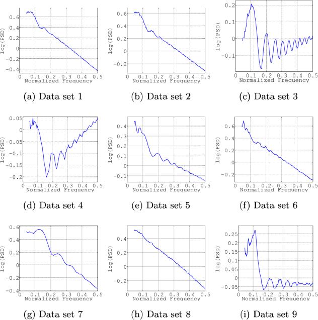
Nine data sets were used in this Challenge, eight consisting of experimentally collected micrographs using a range of samples, microscopes and detectors, while the ninth data set was a collection of computer-simulated images. Table 1 summarizes the number of images in each data set along with some characteristics of the images, including detector, sample, presence of carbon in the imaged area, dose, etc. Additionally, and in order to provide a first estimate of how difficult the task was, we present in Figure 1 examples of representative power spectral densities for the different data sets. (In the Supplementary Material section, Figure Supp-1 shows a more comprehensive description of the data sets.)

Table 1.

Dataset summary.

	Set_1	Set_2	Set_3	Set_4	Set_5	Set_6	Set_7	Set_8	Set_9
Sample (mass)	GroEL (800kDa)	GroEL (800kDa)	60S Ribosome (1.6MDa)	60S Ribosome (1.6MDa)	Apoferritin (500kDa)	Apoferritin (500kDa)	TMV virus	TMV virus	Synthetic Ribosome
Microscope	Tecnai F20	Tecnai F20	Tecnai Polara	Tecnai Polara	Tecnai Polara	JEM3200FSC	CM200 FEG	Tecnai Polara	NA
Detector	TVIPS F415 camera	DE-12	Gatan K2 Summit (counting mode)	Gatan K2 Summit (counting mode)	Film + KZA scanner	DE-12	TVIPS F416 CMOS camera	TVIPS F416 CMOS camera	NA
Grid	minimal carbon	minimal carbon	carbon	no carbon	no carbon	no carbon	holey carbon with minimal carbon	holey carbon with minimal carbon	NA
Voltage (kVolt)	200	200	300	300	200	300	200	300	300
Cs (mm)	2	2	2.26	2.26	2	4.1	2.26	2	2.26
Provided Amplitud Contrast	0.07	0.07	0.1	0.1	0.05	0.1	0.07	0.07	0.1
Sampling (Å/px)	1.38	1.40	1.58	1.58	1.63	1.18	2.19	1.18	1.53
Size (px2)	4096×4096	4086×3062	3712×3712	3712×3712	6070×8050	3062×4086	4096×4096	4096×4096	4096×4096
Part/Density	0.236	0.455	0.415	0.802	0.388	0.716	0.077	NA	0.720
Dose (e/px2)	20	20	22	22	16	20	20	20	NA
Provider	A. Cheng	A. Cheng	J. Frank R. A. Grassucci	J. Frank R. A. Grassucci	R. Henderson S. Chen	W. Chiu J. Jakana	H. Stahlberg M. Chami	H. Stahlberg K. Goldie	J. Frank H.Y.Liao
No. Micrographs	16	16	24	24	17	34	24	34	8

The CTF Challenge requires the estimation of about 200 micrographs grouped in nine datasets. Eight of them contain experimental data (the recording conditions are summarized in the table) and the ninth one is made of simulated data. Part/Density, the particle density, is defined as the average number of particles per micrograph multiplied by the box size that inscribes each particle (in px²) and divided by the micrograph size (in px²). We did not obtain a reliable estimation for dataset 8, which we express by NA.

Figure 1.

Examples of representative power spectral densities for the different data sets. A radial profile is presented in logarithmic scale for each representative. In order to increase contrast, all frequencies smaller than 0.8 (that is, 10 pixels) have been masked out. Note that a downsampling factor of two has been applied to all micrographs before processing, so as to obtain a zoom into the central part of the spectrum. Micrographs have been selected so that they have an average defocus as close as possible to 1.8μ. A more detailed description of the datasets is provided in Supplemental Material

We did not ask the data provider labs for “the best micrographs” they could obtain, but, rather, for micrographs that could indeed be part of an experimental data acquisition session, even having certain “anomalies”. Additionally, we also asked them for their own estimation of the CTF as well as the method they used to estimate it. This information is compiled in Appendix Supp-A.

In data sets 1 and 2, after normal astigmatism adjustment, astigmatism was deliberately introduced by applying extra current to the X objective astigmator to induce 500-1000Å of defocus difference between the two astigmatism directions. Data sets 3 and 4 were acquired on a Gatan K2 camara under over-saturated conditions. This fact translates into a depression of low frequencies. Therefore, when the PSD (Power Spectral Density) is observed and radially averaged, as done in Figure 1, it shows a relative increase at high frequency (this effect is discussed in depth by Li et al. (2013)). In much the same way, data set 7 presents a bias in the experimental CTF estimation performed at the data-producing lab, perhaps because the focusing was done on the thicker carbon film of the Quantifoil grid around two micrometers adjacent to the exposure position. Data set 8, in turn, is especially challenging since the signal-to-noise ratio of the power spectrum density is very low and the Thon rings are barely visible. Finally, CTF profiles in data set 9 have an unexpected property: the CTF radially-averaged profile presents small double peaks at the maxima. This behavior is related to the fact that data set 9 is strongly astigmatic (defocus differences about 10% along the axes) so that each point in the radial profile represents an average over defoci that vary with azimuth.

Results: The Contributions to the CTF Challenge

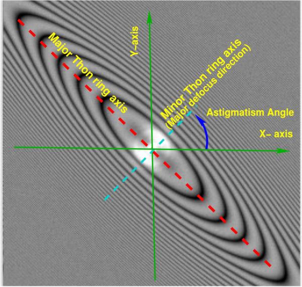
In the CTF Challenge, participants were required to submit estimates of average defocus information and were also encouraged to report on astigmatism. Astigmatism is a lens aberration that causes the defocus to be a function of the azimuthal angle, and is usually defined by 3 parameters: minimum defocus value, maximum defocus value, and the angle between the X-axis and the direction of maximum defocus (see Figure 2 for details).

Figure 2.

Astigmatism is usually denned by 3 parameters: minimum defocus value, maximum defocus value and the angle between the X-axis and the direction of maximum defocus. In the CTF Challenge, the defocus angle is in the range [0, 180), so that a rotation by that angle brings the unit vector (1,0) to coincide with the direction of maximum defocus. In other words, the unit vector with coordinates (cos (astigmatism angle), sin(astigmatism angle)) is parallel to the direction of maximum defocus. Note that the Thon ring major axis is perpendicular to the direction of maximum defocus. Thus, this figure presents an astigmatism angle of +45 degrees.

A total of 21 sets of CTF estimates were uploaded, covering most of the software packages in the field. Participants for 15 of these submissions ranked themselves as “developers” (our highest degree of expertise), 5 as “beginners” (lower level of expertise) and 1 as “expert”.

Data submitted by participants are summarized using a collection of plots presenting the main trends detected in our analysis. In this section we will first present plots showing the average defocus; then, plots related to astigmatism (defocus difference and astigmatism angle); and finally, plots presenting the performance of a new magnitude that measures global CTF discrepancies rather than discrepancies in the estimation of each of its parameters. All these plots clearly show that different data sets behave differently for the task of CTF estimation. Consequently, at the end of the paper, we will split the experimental data sets into two pools, one formed by those data sets with the lowest “discrepancies among the different estimations” and the other one containing those micrographs with the largest “discrepancies” among them, conducting independent observations on each of them. Finally, results will be analyzed in terms of the particular software package that generated them.

Additionally, in Appendix Supp-B the reader may find comments from the Challenge participants on the performance of their particular contributions. The opinions in that appendix express the participants’ personal views and have not been agreed on among the rest of the article authors.

Discrepancy between Uploaded Data and Data Providers’ Estimations

This subsection has three main goals: (1) to describe the type of plots that are going to be used along this work in order to analyze the results collected in the CTF Challenge, (2) to give a first impresion on how disperse these data are and (3), to introduce the concept of “CTF consensus”.

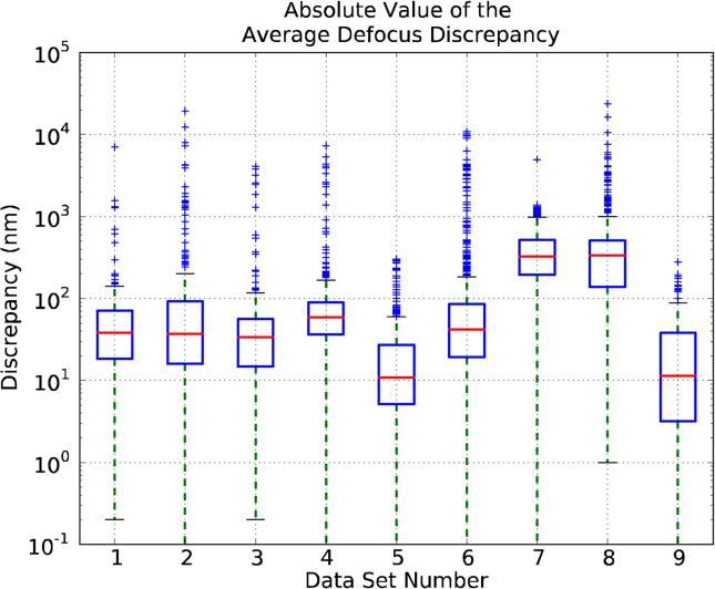
Figure 3 plots the discrepancies between the CTF average defocus values submitted by the participants and the ones estimated by the data providers for the different data sets. This plot, which is in logarithmic scale, uses the so-called “whisker boxplots” that are designed to provide a sense of the data's distribution by plotting the following statistics:

• the bottom and top of the box are the first and third quartiles. The first quartile (designated Ql) splits off the lowest 25% of data from the highest 75%. The third quartile (designated Q3) splits off the highest 25% of data from the lowest 75%

• the band inside the box is the median (also referred as second quartile (Q2)). It cuts the data set in half.

• the two horizontal lines at the end of the green dash lines are called the whiskers. The whiskers mark the lowest datum still within 1.5* (Q3-Ql) of the lower quartile (Ql), and the highest datum still within 1.5 (Q3-Q1) of the upper quartile (Q3).

• finally, outliers (that is, data outside the interval 1.5 * (Q3-Q1) around the median) are plotted as individual small blue horizontal plus signs.

Figure 3.

Comparison of the Average Defocus estimated by the data providers with respect to the one estimated by the participants. X-axis ticks refer to data sets. The bottom and top of the box mark the first (25% of the data) and third quartiles (75% of the data), and the line inside the box marks the second quartile (the median). For a precise definition of Average Defocus Discrepancy, see Appendix B.

Note that the use of a logarithmic scale for the discrepancies is required due to by the relatively large range of the discrepancy values and the desire to show most data points on a single plot. Naturally, it is acknowledged that this representation is less intuitive than a linear one. Also, since the lower whiskers are sometimes very close to 0, the logarithmic scale makes them virtually impossible to be properly represented. We have opted for not plotting those marks in these cases.

Figure 3 presents 9 boxes corresponding to the 9 data sets. For each data set the boxplot contains information for all the uploads made by each participant. For example, since there are 21 uploads and 16 micrographs in data set 1, around 546 values are used to compute the first box. The number is not exactly 546 because a few uploads have not estimated all the micrographs.

The discrepancies shown in Figure 3 assume that the CTF estimation performed by the data providers is essentially correct, but this assumption is not supported by any quantitative data. In particular, there is a clear inconsistency for data set 7, presenting most of the outliers grouped in a cluster outside the box, suggesting that there was a bias in the data provider's defocus estimation (this bias is probably related to the fact that defocus was estimated focusing on a grid position adjacent to the area in which the micrographs were actually taken (see Appendix Supp-A)). Additionally, many CTF estimations given by the data providers were based on Ctffind, and their direct use might introduce a bias toward this particular method. Therefore, we decided to change the reference used to calculate the discrepancies from the values reported by the data providers to a new “synthetic measurement”, which we will here refer to as “Consensus Value”. The Consensus Values are defined as the average of the estimations by all participants excluding the outliers (see Appendix B for further details). We wish to note that we do not attach any especial meaning to this Consensus Value, and grant that it may be a biased estimator. Still, using multiple algorithms to estimate defocus seems to be a safer approach than to rely on just a single one. Indeed, there are applications, such as classification, in which combining multiple algorithms has been shown to perform well (Kuncheva, 2004).

Discrepancy between Uploaded Data and Consensus Values

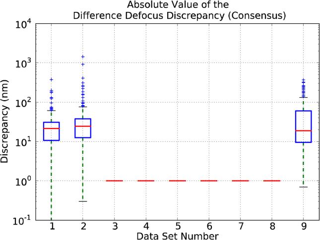
In this subsection we will analyze in detail the discrepancies found between the different CTF estimations provided by the Challenge participants and the Consensus Values. In this way, Figure 4 is similar to Figure 3, but using the Consensus Values as a reference. Results do not change much in between the two Figures, except for data sets 7 and 8 and, to a lesser extent, data sets 3 and 4. The changes for data set 7 are easily explainable in terms of a defocus estimation bias. At the same time, it is clear that for data set 8 the discrepancies among the different estimations are very large (Q3 amounts to several hundred nanometers) and, indeed, Thon rings are barely visible (Figure Supp-1); at this point we decided to exclude data set 8 from subsequent studies, as it clearly presents a case for which no reliable CTF estimation can be currently performed. The situation for the other data sets is simpler, indicating that in most cases the Consensus Values for the average defocus and the one supplied by the data providers were not very different, with data sets 3 and 4 being the ones with larger differences. As a general remark, we can note that there are large differences among the discrepancies reported for the different data sets, with the average of their means being around 30 nm and with a large number of outliers.

Figure 4.

As Figure 3, but using the Consensus Defocus as reference value instead of the estimation provided by the data providers.

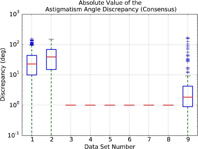
As far as astigmatism is concerned, we only report results for the Difference Defocus Discrepancy and for the Astigmatismm Angle Discrepancy (see Appendix B) for data sets 1, 2 and 9, since these are the ones with noticeable astigmatism as reported by the data providers. Figure 5 shows the discrepancy in the estimation of the defocus difference, while Figure 6 refers to the astigmatism angle. As can be observed in Figure 5, the medians for the Difference Defocus Discrepancy are around 25, 30 and 20 nm for data sets 1, 2 and 9, respectively. In much the same way, the medians for the Astigmatism Angle Discrepancy are close to 25°, 40° and 2° (Figure 6).

Figure 5.

Comparison of the Defocus Difference Discrepancy estimated by the participants with respect to the Consensus. X-axis ticks refer to data sets. For a precise definition of Defocus Difference Discrepancy, see Appendix B. We only report results for data sets 1, 2 and 9, since theses are the ones with noticeable astigmatism.

Figure 6.

Comparison of the Astigmatism Angle Discrepancy estimated by the participants with respect to the Consensus. X-axis ticks refer to data sets. For a precise definition of Astigmatism Angle Discrepancy, see Appendix B. We only report results for data sets 1, 2 and 9, since theses are the ones with noticeable astigmatism.

Naturally, these median values are to be understood in the context of the variable being measured, especially for the Astigmatism Angle Discrepancy. In this case, it is probably intuitive that a value for the median of the discrepancy of just 2 degree -data set 9- is very good, but it is not so clear for data set 1 and, especially, for data set 2, whose median discrepancy is up to 40°. In other words, an objective test is needed to discard the hypothesis that the astigmatism angle estimations (both for the values provided by the participants and by the data providers) are better than the ones obtained using random values. Therefore, we should compare the statistics of the distribution of the absolute difference of one random uniform variable (the upload) and a sum of random uniform variables (the Consensus). Making the simplification that the Consensus behaves just as a random variable, the problem reduces to a Triangular distribution (Evans and Peacock, 2000; Wikipedia, 2014) with lower limit 0, upper limit 180 and mode 0, for which the predicted value for the median (Q2) is equal to 52° and the upper quartile (Q3) is 90°. Consequently, we may conclude that, indeed, the estimation of the astigmatism angle for data sets 1 and 9 is providing quite valuable information, but that for data set 2 the distribution of the estimations in the different uploads is close to random, though still statistically different from random.

An interesting situation is illustrated by data set 9, composed of computer-generated images with a relatively large astigmatism (10% defocus difference) for which, of course, the precise CTF parameters are known. As noted before, the median of the Astigmatism Angle Discrepancy is indeed very small, and it is tempting to assume that this good behavior is going to repeat when analysing other CTF parameters. However, this is clearly not the case since, the Average Defocus estimations for this data set, although good, are not the best ones, that corresponds to data set 5 (see Figure 4 for details).

Influence of the CTF Estimation Discrepancy in the 3D map Resolution

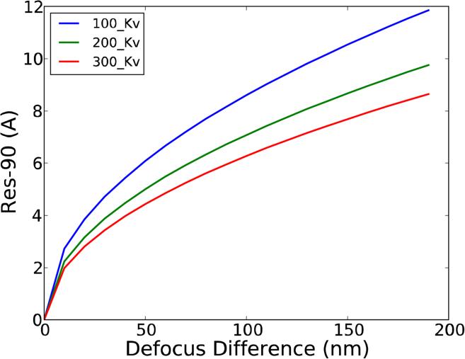
A natural question to be posed at this point is how to characterize the relationship between a given discrepancy in the CTF estimation for a micrograph and the quality of the structural information that can be extracted from it. Focusing on resolution, in Figure 7 we display, as a function of acceleration voltage and defocus difference, the maximum resolution up to which two (non-astigmatic) CTF estimations would be “equivalent”, denning “equivalent” as having a wave aberration function shift smaller than 90° (wave aberration function is defined in Appendix B). We will refer to this resolution limit as Res-90. It is to be noted that “maximum achievable structural resolution” -a term somehow difficult to define- is not the same as Res-90, since, for example, on the positive side, after 90° shift still some information can be extracted and, on the negative side, in the neighborhood of the CTF zeros the transfer of information is very sensitive to the precise defocus estimate. Still, Res-90 is a magnitude that can be quantitatively denned in a simple manner in a variety of situations, allowing interpretation and comparison of the effect of CTF estimation errors upon structural resolution.

Figure 7.

Resolution at which the wave aberration shift introduced by a given defocus error is 90°. Note that this magnitude depends only on the defocus error and not on the actual amount of defocus. Additionally, note that the plot would be the same if instead of considering two non-astigmatic CTF estimations we would consider the defocus difference between the two astigmatic axis, assuming no errors in astigmatic angle estimation.

In this way, for example, a difference of 50 nm in defocus translates into a change of 90° in the CTF phase at around 4Å at 300 kV, and into 6Å at 100 kV, but only if we did not have additional errors in defocus average and astigmatism estimation. Since actually we have large errors in astigmatism estimation, the resolution limit will be somewhat worse. Furthermore, Res-90 can be generalized (see Appendix B) so as to take into account in a very concise manner -by one single number- errors in defocus difference as well as astigmatism angle, resulting into a new figure that we will refer to as RES-90 (with capital letters), which will be extensively used in the following sections. Note that we will consider the Consensus defocus for the calculation of RES-90. In short, RES-90 takes into account errors in defocus magnitude and astigmatism directions into a single figure that is related (but not equal to) to the maximum resolution achievable with that data set for a given CTF estimation.

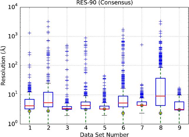
Figure 8 displays the average and standard deviation of RES-90 for all data sets and uploads. For each data set the yellow circles mark Nyquist resolution (that is, the pixel size at the specimen level multiplied by 2). Focusing first on RES-90 median values, data sets 3, 5, and 7 have values close to Nyquist, while data sets 1 and 4 are between 4 and 5Å, with the rest of the experimental data sets (2 and 6) being between 5 and 6Å. Regarding values above the upper quartile (Q3) -the upper limit of the box- (which we recall, are provided per data set), they are in general large. Indeed, if we now choose to select as quality criterion the Q3 limit for a particular data set (in other words, that 75% of all CTF estimations on that data set gave a lower RES-90 value), only two data sets would be below 4Å (data sets 3 and 5), and another two in the range 4-6Å (data sets 4 and 7). Of course, any further inaccuracies in image processing can only lower the final maximum achievable resolution. Note, additionally, that the trend is that data sets with a lower RES-90 median value (data sets 3, 5 and 7) also have a lower Q3, implying that the micrographs for those data sets behave in a similar way for the different uploads. Finally, RES-90 for the computer generated images (data set 9) is alike to the experimental data sets, indicating similar errors in the CTF estimation. In all cases the number of CTF estimations that can be considered “outliers” (they present very significant deviations with respect to the Consensus Values) is not negligible.

Figure 8.

RES-90 analysis. X-axis ticks refer to data sets, Y-axis represents an estimation of the resolution limit imposed by the accuracy in the CTF determination. Yellow circles show the Nyquist frequency for each data set.

Performance of CTF estimation using different Software Packages

An interesting, although complex question to be asked at this stage is whether the different software packages are equally good in estimating the CTF. When comparing results, we must bear in mind that not all participants have submitted estimations for all micrographs and that some contributions have not been provided by the package developers. In fact, we list in Table Supp-1 the number of micrographs processed for each upload, noting that most of the uploads contain all 197 micrographs (i.e. upload 282), but that there are cases in which only a small subset has been processed (i.e. upload 303 -with data for only 16 micrographs, all of them belonging to data set 1-). Since previous figures clearly show that different data sets behave differently for the task of CTF estimation, for the following studies we have decided to split the experimental data sets into two pools. The first one formed by data sets 3, 4, 5 and 7 (Pool 1), and the other by data sets 1, 2, 6 (Pool 2) (data set 8 was disregarded in this analysis, since its discrepancies were too large). Pool 1 is consider to be less challenging than Pool 2 from the point of view of CTF estimation.

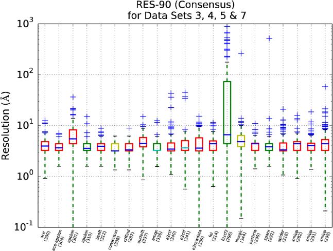
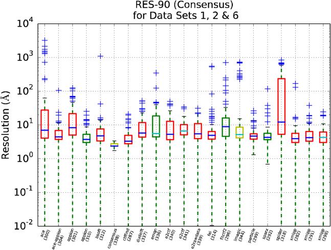
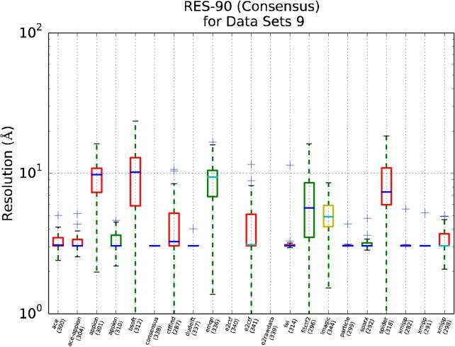
We present in Figures 9, 10 and 11 RES-90 for Pool 1, Pool 2 and for the synthetic data set, respectively. In these figures, (1) the results are grouped by package name rather than by data sets, (2) the median is colored blue for those uploads that have estimated all the CTFs, and cyan otherwise and, (3) the box color is related to the participant's own stated level of expertise, with red being the highest, yellow intermediate and green the lowest.

Figure 9.

RES-90 as a function of the package used in the upload (the upload id number is provided in parenthesis). This plot only uses data sets 3, 4, 5 and 7, which are the ones with the smaller discrepancies. The box color is related to the participant's own stated level of expertise, with red being the highest, yellow intermediate and green the lowest. The median is colored dark blue for those uploads that have estimated all the CTFs and cyan otherwise.

Figure 10.

RES-90 as a function of the package used in the upload. This plot only uses data sets 1, 2 and 6 which are the ones with larger discrepancies (the upload id number is provided in parenthesis). The box color is related to the participant's own stated level of expertise, with red being the highest, yellow intermediate and green the lowest. The median is colored dark blue for those uploads that have estimated all the CTFs and cyan otherwise.

Figure 11.

RES-90 as a function of the package used in the upload (the upload id number is provided in parenthesis). This plot only uses data set 9, the synthetic one. The box color is related to the participant's own stated level of expertise, with red being the highest, yellow intermediate and green the lowest. The median is colored dark blue for those uploads that have estimated all the CTFs and cyan otherwise. Note that some uploads did not contain information related with data set 9 and therefore no boxplot has been drawn.

From Figures 9 and 10 we may conclude that for Pool 1 many software packages produce similar results, while for Pool 2 the situation is more confused. This result may be interpreted in a qualitative manner indicating that for those data sets with higher quality images (Pool 1), most CTF estimation methods work similarly; however, when the images are more challenging (Pool 2), there are clear differences among the different methods. Still, beyond the previous general statement, it is difficult to derive conclusions from Figures 9 and 10 directly, mostly because of the complex distribution of the values being plotted, and more precise and quantitative statistical analysis had to be performed on the data to derive ranking information. In the next sections we will proceed further in this analysis following a two-step approach: first, we will test the claim that two populations (i.e. uploads) are different and, then, we will rank the performance of each upload with respect to the other.

Step 1: Comparing Populations

A T-test can be used to determine if the means of two sets of data are significantly different from each other providing that the population follows a normal distribution. An alternative for non-normal populations (as our case) is the so called Wilcoxon signed rank test (Siegel, 1988).

Wilcoxon tests were computed for all pairs of uploads. Figures Supp-3, Supp-4, Supp-5 and Supp-6 show the result of performing this test when grouping the data in four different ways: (1) all experimental data sets (except for data set 8), (2) Pool 1, (3) Pool 2 and (4) the synthetic data set. In the following, and as it is the standard procedure in statistics, we will consider two uploads to be different if their corresponding p-value is smaller than 0.05.

Focusing on the uploads related to the best performing packages (how this ranking has been obtained is described in the next section), it is straight-forward to deduce that the difference of the top ranking upload (upload 287, Ctffind3) for the groups composed of (1) all experimental data sets and (2) Pool 1, is statistically significant when compared with any other upload. On the other hand, for Pool 2 we cannot reject the hypothesis that upload 287 (Ctffind3) and upload 310 (Appion) provide similar results, but we can reject this hypothesis for the rest of the uploads. Finally, the situation is different with the synthetic data, were half of the uploads performs equally good (Figure Supp-6).

Step 2: Ranking

Once we know which uploads are statiscally different, we can rank the uploads using RES-90. To achieve this ranking we will follow an Analytic Hierarchy Process approach (Saaty, 1988). This methodology has been quite successful in Decision Making, finding applicability in many scientific fields. Note that this ranking does not provide an indication on how much better a method is compared to other.

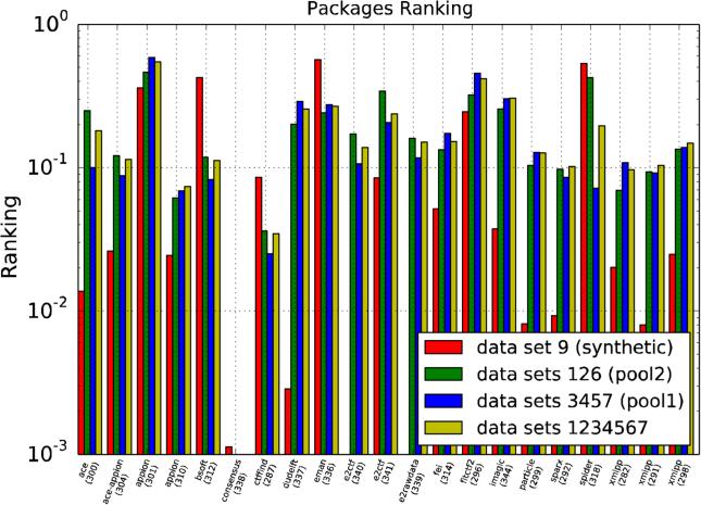
Figure 12 and Table 2 show the result of this comparison for all experimental data sets (except for data set 8), Pool 1, Pool 2 and the synthetic data set, respectively. It is clear that most methods behave much better for the synthetic data set than for any of the experimental ones, with the exception of Ctffind. This exception may be particularly interesting because the plots also indicate that Ctffind is the highest-ranked method for Pool 1 and (together with Appion) for Pool 2. In contrast, note also that the software by the University of Delft is certainly among the best ones for the synthetic data set, but that it ranks low for all experimental data sets.

Figure 12.

Comparison for all experimental data sets (but data set 8), Pool 1, Pool 2 and the synthetic data set respectively. X-label color refers to the participant expertise level.

Table 2.

Upload ranking for the different data sets.

#	data sets 9	data sets 1,2&6 Pool 2	data sets 3,4,5&7 Pool 1	data sets 1, 2, 3, 4, 5, 6 & 7
1	dudelft (337)	ctffind(287)	ctffind(287)	ctffind(287)
2	xmipp(291)	appion(310)	appion(310)	appion(310)
3	particle(299)	xmipp(282)	spider(318)	xmipp(282)
4	sparx(292)	xmipp(291)	bsoft(312)	sparx(292)
5	ace(300)	sparx(292)	sparx(292)	xmipp(291)
6	xmipp(282)	particle(299)	ace-appion(304)	bsoft(312)
7	appion(310)	bsoft(312)	xmipp(291)	ace-appion(304)
8	xmipp(298)	ace-appion(304)	ace(300)	particle(299)
9	ace-appion(304)	fei(314)	e2ctf(340)g	e2ctf(340)
10	imagic(344)	xmipp(298)c	xmipp(282)	xmipp(298)
11	fei(314)	e2rawdata(339)	e2rawdata(339)	e2rawdata(339)
12	e2ctf(341)	e2ctf(340)d	particle(299)	fei(314)
13	ctffind(287)	dudelft (337)	xmipp(298)	ace(300)
14	fitctf2(296)	eman(336)e	fei(314)	spider(318)
15	appion(301)	ace(300)	e2ctf(341)	e2ctf(341)
16	bsoft(312)	imagic(344)f	email (336)h	dudelft (337)
17	spider(318)	fitctf2(296)	dudelft (337)	eman(336)
18	eman(336)	e2ctf(341)	imagic(344)	imagic(344)
19	e2ctf(340)a	spider(318)	fitctf2(296)	fitctf2(296)
20	e2rawdata(339)b	appion(301)	appion(301)	appion(301)

Color refers to the participant expertise level; Those packages followed by a super scripted character have not uploaded all the micrographs proposed in the challenge (see details at the caption end). For data set 9, the performance of the top ranking upload (upload 337, dudelft) is indistinguishable from the performance of all the uploads in rows 2 to 9 -that is, Wilcoxon test does not reject the hypothesis that upload 337 is different from uploads 291, 299, etc.- For data sets 1, 2 & 6 (Pool 2), the performance of the top ranking upload (upload 287, ctffind) and the second one (upload 310, appion) is indistinguishable. For data sets 3, 4. 5 & 7 (Pool 1) and also for data sets 1, 2, 3, 4, 5, 6 & 7, the performance of the top ranking upload (upload 287, ctffind) is better than the performance of any other upload. Notes:

^aupload 340 did not upload information for data set 9

^bupload 339 did not upload information for data set 9

^cupload 298 did not upload information for data set 6

^dupload 340 did not upload information for some data sets 1 and 2

^eupload 336 did not upload information for data sets 1 and 2

^fupload 334 did not upload information for some micrographs

^gupload 340 did not upload information for data set 7

^hupload 336 uploaded data information for set 5 only.

Discussion

The accurate determination of the CTF parameters of sets of electron micrographs is a challenging task because of the large variation in image acquisition conditions (film/scanner combinations, CCD's with different phosphors, direct detectors, etc.), variation in the image content (with/without carbon, ice thickness, particle sizes) and extraneous factors (micrograph edges, micrograph number panels, dirt on films or detectors, etc.) that may occur in normal practice. Consequently, it is important to compare the different estimation methods in a wide range of conditions. The main contribution of this work is collecting and making available a representative set of micrographs, as well as performing a first analysis on a large number of contributions covering most software packages in the field.

As a rule, and certainly not unexpectedly, estimations of average defocus are much better than astigmatism estimations. Judging by the consistency among many independent CTF estimations on the same sets, we can roughly estimate that the third quartile (i.e. corresponding to 75% of the micrographs) of the average defocus estimation discrepancies are lower than 30 nm for the best data sets, and up to 60 nm for the more challenging ones, with no obvious dependency on the defocus range.

As far as astigmatism is concerned, we have found discrepancies in average defocus range between 20 to 60 nm. However, regarding astigmatism angle determination, we have shown how its estimation by the different methods have large discrepancies, although it is still statistically better than random. This fact suggests that astigmatism detection is not yet well enough implemented in CTF estimation methods. Consequently, in our quest for high resolution, images should be screened first to get rid of any noticeable astigmatism, before CTF estimation methods are used to detect angles and small defocus differences, for which probably the estimation errors will be large. These astigmatism-related errors have, therefore, an impact in high resolution (Figure 7) and cannot be neglected.

A very clear trend can be recognized when a data set is especially well suited for high resolution (as, for instance, judged by RES-90), and it is that most software packages provide similar estimations for the CTF parameters. In other words, when a data set is “good”, most packages provide similar results.

It is interesting to note that among the best data sets (Pool 1) two of them have carbon support and two do not. Furthermore, the particle density (i.e., the number of particles per area) is quite different among the micrographs. Therefore, it seems that the presence or absence of carbon and the particle density are not per se determining the quality of the CTF estimations. Indeed, most of the better data sets do not have carbon, and one of the best (data set 5) does not have a particularly large density of particles. Consequently, we consider that this is a question to be further addressed by analyzing far larger sets than the ones compiled here.

Regarding recording media, the data sets for which the CTF estimation presented smaller discrepancies were obtained in the following way: two on DDD's (K2), one on film and the fourth one on a CMOS camera. Interestingly, the over-exposure of the images in data sets 3 and 4 did not preclude an accurate CTF determination, in the sense that most algorithms behave very well on them, although the final quality of further structural analysis would be compromised.

The behavior of synthetic data deserves a detailed analysis. On the one hand, most distributions of discrepancy measurements were similar for this data set and for the experimental data sets. On the other hand, the ranking of the software packages based on synthetic data is quite different from the one based on experimental data. Furthermore, some parameters were determined with high precision for the computer-simulated images, while others were not; this is the case of the very good performance for Astigmatism Angle estimation but not for Average Defocus or for Defocus Difference. It is difficult to know if this behavior is a shortcoming of current synthetic image data generation or if other factors are also present, such as the amplitude contrast, but it clearly highlights the obvious need to work with very different data sets in order to properly test any development.

Regarding software packages, it is difficult to extract broad-range conclusions in view of the limited number of uploads per package (normally only one) and the diversity of the data treated in each of them, as indicated in Table 1. Therefore, great care should be used not to overinterpret Figure 12. Still, we may conclude that CTFFIND3 consistently excels, except, somehow unexpectedly, for the synthetic data set.

We hope that this Challenge contributes to establishing a dynamic of algorithmic benchmarking. In the spirit of this idea, the images used in this challenge together with the associated consensus estimations are available to all interested users at URL http://i2pc.cnb.csic.es/3dembencrimark/LoadCtfInformation.htm.

A CTF Description

In the following we introduce the parametric form used to describe the CTF assumed in the CTF Challenge. In particular, note that there is no term describing the CTF damping.

$$\begin{array}{cc}\hfill CTF\left(\mathbf{R}\right)=& w\cos \left(\gamma \left(\mathbf{R}\right)\right)-\sqrt{1-w^2}\sin \left(\gamma \left(\mathbf{R}\right)\right)\hfill \\ \hfill \gamma \left(\mathbf{R}\right)=& 180\lambda (-\Delta Z\left(\angle \mathbf{R}\right){\Vert \mathbf{R}\Vert }^2+\frac{Cs{10}^6{\Vert \mathbf{R}\Vert }^4{\lambda }^2}{2})indegrees\hfill \\ \hfill \Delta Z\left(\angle \mathbf{R}\right)=& Z_{avg}+Z_{diff}\cos \left(2(\angle \mathbf{R}-ϴ)\right)innm.\hfill \\ \hfill \Delta Z_{avg}=& \frac{Z_{max}+Z_{min}}{2}\hfill \\ \hfill \Delta Z_{diff}=& \frac{Z_{max}-Z_{min}}{2}\hfill \end{array}$$

where R is the 2D spatial frequency, ΔZ denotes defocus, $\angle \mathbf{R}$ is the angle between the X axis and the vector defined by R, Θ is the astigmatism angle (angle between the direction of maximum defocus and the X axis), w is the percentage of amplitude contrast and Cs is the spherical aberration in mm. Finally, the factor 10⁶ converts Cs from mm to nm and γ(R) is termed in the specialized literature as wave aberration function.

B Description of the Magnitudes Plotted in this Work

In the different figures along this article we report on the average (Y-axis value) and standard deviation (error bar) for the following magnitude.

• $defocusAverageDiscrepancy=\mid \frac{(Z_{max}+Z_{min})-(Z_{max}^0+Z_{min}^0)}{2}\mid$

• $defocusDiffDiscrepancy=\mid \frac{(Z_{max}-Z_{min})-(Z_{max}^0-Z_{min}^0)}{2}\mid$

• $angleDefocusDiscrepancy=\mid ϴ-{ϴ}_0\mid$ where the subindex 0 refers to the “reference” estimation, which is either the one provided by the data providers or the “consensus value”, which is defined in the following way:

  1. For each micrograph, the mean and standard deviation of the defocus average are computed.
  2. Outliers are defined as points further away than two times the standard deviation from the mean and are then removed.
  3. Mean for all CTF parameters are now re-calculated from the remaining data.
  4. “Consensus value” is defined as this new mean value.

• RES-90 = Spatial frequency at which the wave aberration functions created using the uploaded parameters and the “reference” ones differ by 90° (a detailed explanation is provided below).

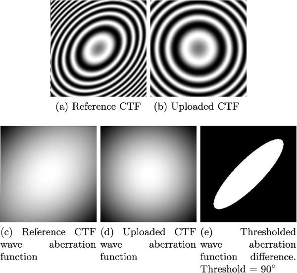
RES-90 computation assumes that $CTF\left(\mathbf{R}\right)=w\cos \left(\gamma \left(\mathbf{R}\right)\right)-\sqrt{1-w^2}\sin \left(\gamma \left(\mathbf{R}\right)\right)$ and it is calculated as follows (see Figure 13):

1. The wave aberration function (that is, γ in the above equation) is computed for the reference and the uploaded CTF (see Figures 13c and 13d).

2. A 2D image is produced from the astigmatic wave aberration function for both the reference and uploaded CTF parameters

3. The two resulting images are subtracted, creating a difference image.

4. The difference image is thresholded at 90° (see Figure 13e).

5. The number of white pixels in the thresholded area is counted.

6. A “mean” resolution R is then computed as the radius of the circle that has the same number of pixels (πR²) than those obtained in the previous step.

7. The radius is transformed from pixels to angstroms, resulting in RES-90.

Figure 13.

Summary of the steps followed to compute RES-90. (a) and (b) show an example of the reference and the uploaded CTFs. (c) and (d) show the CTF wave aberration function (γ((R))) for the reference and uploaded CTFs. (e) shows the difference between (c) and (d) after binarization: all values greater than 90° are set to 0, all values smaller are set to 1.

References

- Evans M, Hastings N, Peacock B. Statistical Distributions. Ch. Triangular Distribution; Wiley, New York: 2000. pp. 187–188. [Google Scholar]
- Kuncheva LI. Combining Pattern Classifiers: Methods and Algorithms. Wiley-Interscience; 2004. [Google Scholar]
- Li X, Zheng SQ, Egami K, Agard DA, Cheng Y. Influence of electron dose rate on electron counting images recorded with the K2 camera. J. Struct. Biol. 2013 Nov;184(2):251–260. doi: 10.1016/j.jsb.2013.08.005. [DOI] [PMC free article] [PubMed] [Google Scholar]
- Ludtke SJ, Lawson CL, Kleywegt GJ, Berman H, Chiu W. The 2010 cryo-em modeling challenge. Biopolymers. 2012;97(9):651–654. doi: 10.1002/bip.22081. [DOI] [PubMed] [Google Scholar]
- Saaty T. What is the analytic hierarchy process? In: Mitra G, Greenberg H, Lootsma F, Rijkaert M, Zimmermann H, editors. Mathematical Models for Decision Support. Vol. 48 of NATO ASI Series. Springer; Berlin Heidelberg: 1988. pp. 109–121. URL http://dx.doi.org/10.1007/978-3-642-83555-1_5. [Google Scholar]
- Siegel S. Nonparametric statistics for the behavioral sciences. McGraw-Hill; 1988. [Google Scholar]
- Smith R, Ventura D, Prince JT. Novel algorithms and the benefits of comparative validation. Bioinformatics. 2013 doi: 10.1093/bioinformatics/btt176. [DOI] [PubMed] [Google Scholar]
- Wikipedia [17-July-2014];Triangular distribution – Wikipedia, the free encyclopedia. 2014 URL http://en.wikipedia.org/wiki/Triangular_distribution# Distribution_of_the_absolute_difference_of_two_standard_uniform_variables.
- Zhu Y, Carragher B, Glaeser RM, Fellmann D, Bajaj C, Bern M, Mouche F, de Haas F, Hall RJ, Kriegman DJ, Ludtke SJ, Mallick SP, Penczek PA, Roseman AM, Sigworth FJ, Volk-mann N, Potter CS. Automatic particle selection: results of a comparative study. J. Struct. Biol. 2004;145(1-2):3–14. doi: 10.1016/j.jsb.2003.09.033. [DOI] [PubMed] [Google Scholar]
Associated Data
This section collects any data citations, data availability statements, or supplementary materials included in this article.