A Bayesian Nonlinear Mixed-Effects Regression Model for the Characterization of Early Bactericidal Activity of Tuberculosis Drugs

Abstract

Trials of the early bactericidal activity (EBA) of tuberculosis (TB) treatments assess the decline, during the first few days to weeks of treatment, in colony forming unit (CFU) count of Mycobacterium tuberculosis in the sputum of patients with smear-microscopy-positive pulmonary TB. Profiles over time of CFU data have conventionally been modeled using linear, bilinear, or bi-exponential regression. We propose a new biphasic nonlinear regression model for CFU data that comprises linear and bilinear regression models as special cases and is more flexible than bi-exponential regression models. A Bayesian nonlinear mixed-effects (NLME) regression model is fitted jointly to the data of all patients from a trial, and statistical inference about the mean EBA of TB treatments is based on the Bayesian NLME regression model. The posterior predictive distribution of relevant slope parameters of the Bayesian NLME regression model provides insight into the nature of the EBA of TB treatments; specifically, the posterior predictive distribution allows one to judge whether treatments are associated with monolinear or bilinear decline of log(CFU) count, and whether CFU count initially decreases fast, followed by a slower rate of decrease, or vice versa.

1. INTRODUCTION

1.1. Early Development of Tuberculosis Treatment Regimens

Standard efficacy endpoints in pivotal Phase III trials of tuberculosis (TB) treatments are the proportion of patients with positive sputum culture after 6 months of treatment, and the proportion of patients experiencing relapse within a 2-year follow-up period (Mitchison, 2006; Mitchison and Davies, 2008). Proof of clinical efficacy of TB treatments, therefore, generally requires lengthy and expensive clinical trials (Mitchison, 2006; Phillips and Fielding, 2008; Wallis et al., 2009). Furthermore, mono-therapy with anti-TB drugs is often ineffective, mainly due to increasing incidence of drug resistance (Yang et al., 2011), so that TB is typically treated with combinations of bactericidal and sterilizing drugs (Diacon et al., 2012). As Diacon et al. (2012) state, “ideally [new treatment] regimens would contain new drugs able to combat tuberculosis resistant to currently available drugs, especially multidrug-resistant (MDR) tuberculosis….” Thus one of the challenges in early development of new TB treatments is to identify promising combinations of drugs for subsequent testing in pivotal clinical trials. Since the treatment regimens may involve combinations of three or four drugs, including one or more novel molecules, potentially large numbers of regimens need to be screened. One way to do so efficiently and cost-effectively is to assess the early bactericidal activity (EBA) of those regimens.

1.2. Early Bactericidal Activity

An EBA trial assesses the decline, during the first few days to weeks of treatment, in colony forming unit (CFU) count of Mycobacterium tuberculosis in the sputum of patients with smear-microscopy-positive pulmonary TB (Diacon et al., 2012). Such EBA trials are usually conducted during the early stage of drug development (Phase II).

An early definition of EBA was the “fall in counts/mL sputum/day [of CFU count] during the first two days of treatment” (Mitchison and Sturm (1997) as cited in Donald and Diacon (2008)). More generally, the EBA in a given patient over a time interval from Day t ₁ to Day t ₂, i.e. EBA (t ₁ – t ₂), can be estimated as follows:

(1)

(see, e.g. Botha et al. (1996)). Here, and are the observed log(CFU)counts at Day t ₁ and Day t ₂, respectively, where , and T is the length of the profile period over which serial sputum samples are collected. Equation (1) represents a “model-free” estimate of EBA(t ₁ – t ₂), since it is the function only of the observed log(CFU) counts at Day t ₁ and Day t ₂.

Alternatively, EBA(t ₁ − t ₂) can be estimated as:

(2)

where f(t) is a suitable regression function for log(CFU) count vs. time, and and are the associated fitted values at Day t ₁ and Day t ₂, respectively (see, e.g. Jindani et al. (2003)).

The model-based estimate of in Equation (2) has two potential advantages over the model-free estimate in Equation (1): First, the EBA estimate in Equation (1) uses information from only two CFU counts, namely those observed at Day t ₁ and Day t ₂; in contrast, the whole series of observed CFU counts may be used to estimate and , with potential gains in precision for the model-based EBA estimate in Equation (2). Second, the model-free EBA estimate for a given time interval (t ₁ – t ₂) can only be calculated if CFU counts are in fact available for these particular times; in contrast, the model-based estimate can be calculated (e.g. by extrapolating the curve over time interval (t ₁ – t ₂)) even if CFU counts have not been observed at Day t ₁ and Day t ₂, either because the study design did not specify data collection at those times or because of missing data.

We note that, if the regression function f(t) is linear over the whole profile period [0, T], then the EBA estimate in Equation (2) is given by minus one times the slope of the regression of log(CFU) count against time. Indeed, both in vitro and in vivo studies have suggested that anti-TB drugs eradicate a fixed proportion of TB bacteria per unit time (Gillespie et al., 2002), at least over suitably short time intervals, which would imply an exponential decay in CFU count, or equivalently, a linear decay in log(CFU) count. Thus, if the decay of CFU counts over the whole interval [0, T] is exponential (equivalently, log-linear), the EBA estimate in Equation (2) over all sub-intervals (t ₁ – t ₂) of [0, T] is constant and equal to minus one times the slope of the linear regression line of log(CFU) count vs. time.

1.3. Need for Nonlinear Regression Models

Jindani et al. (2003) argued that “standard EBA” TB trials, namely those estimating EBA(0–2), may fail to measure the sterilizing activity of TB drugs: For example, mono-therapy of pyrazinamide has been shown to be less bactericidal than that of isoniazid and streptomycin during the first few days of treatment (EBA), but proves to eradicate TB bacteria at about the same rate afterward (sterilization). Thus, even though pyrazinamide has weak EBA, its sterilizing activity proves to be better than that of isoniazid and streptomycin (Brindle et al., 2001; O’Brien, 2002). Based on these findings, Jindani et al. (2003) suggested the extension of “standard EBA” trials to a treatment period of at least 5 to 7 days, in order to evaluate the sterilization activity of anti-TB drugs. Currently, the treatment and profile period for EBA trials typically is 14 days, with collection of one or two pretreatment and serial post-treatment overnight sputum samples. EBA values that are routinely reported for such TB trials include EBA(0–2), EBA(0–14), EBA(2–14), and EBA(7–14).

As mentioned above, over a suitably short time interval, a TB drug typically eradicates a fixed proportion of TB bacteria per unit time, implying exponential decline of CFU count over the time interval in question. Empirically, an exponential decline of CFU count (or a linear decline in log(CFU) count) has indeed been observed for most TB regimens, at least during the first few days of treatment, and certainly during the first two days. Thus, EBA(0–2) can be estimated from a simple linear regression of log(CFU) count vs. time (see Equation (2)) (Brindle et al., 2001; Jindani et al., 2003; Dietze et al., 2008). However, when the profile period of EBA trials, and associated EBA calculations, covers time intervals significantly longer than 2 days, say 14 days, then the assumption of a constant rate of decay over the whole time interval generally is no longer valid. In fact, for many TB drugs, a significant difference between the rate of decline over the first two days of treatment compared to the subsequent days has been observed (Donald and Diacon, 2008): Usually, during the first few days of treatment, log(CFU) counts decline with a fast rate, followed by a slower rate of decline during the second phase. The decline in log(CFU) count can therefore be biphasic (Mitchison and Davies, 2008) over a 14-day treatment period. Thus, for EBA trials with longer profile periods, estimation of EBA generally requires some form of nonlinear modeling that appropriately reflects the biphasic nature of the regression of log(CFU) count against time.

1.4. Nonlinear Regression Models Proposed in Literature

In order to account for the biphasic nature of log(CFU) count vs. time curves, two types of nonlinear regression models have essentially been described in the literature, namely bilinear and bi-exponential regression.

Diacon et al. (2012, 2013) performed bilinear regression of log(CFU) count against time on a by-patient basis, with visual identification of the node parameter (or inflection point), and assuming that the node was the same for all patients in a given treatment group. Thus, the approach of Diacon et al. (2012, 2013) did not accommodate between-patient variation in the node. Accordingly, EBA was compared between treatment groups using analysis of variance of the resulting by-patient EBA estimates. Furthermore, it would seem preferable to estimate the node parameter from the data, rather than determine it through visual inspection. In addition, it would seem preferable to fit the model as a bilinear mixed-effects regression model.

Jindani et al. (2003) suggested that the switch of one rate of decline in log(CFU) count to another might be smooth (rather than abrupt, as would be implied with a bilinear regression model). Modeling such a smooth transition, Gillespie et al. (2002) and Jindani et al. (2003) used bi-exponential regression of CFU count against time, while Davies et al. (2006a), Davies et al. (2006b), and Rustomjee et al. (2008) regressed log(CFU) count, observed over 56 days of treatment, against the logarithm of a bi-exponential function as a mixed-effects regression model. However, in bi-exponential regression models, the initial rate of decline in CFU count necessarily is greater than the terminal rate. Thus, bi-exponential regression models do not seem adequate for treatments (and individual profiles) which are associated with terminal rates of decline that are faster than initial rates of decline. Such treatments have only been described recently (Diacon et al., 2012). The bi-exponential mixed-effects regression model can fit data beyond 14 days of treatment, e.g. for 56-day “serial sputum colony counts (SSCC)” trials (Rustomjee et al., 2008). The trial discussed by Rustomjee et al. (2008) shows a clear distinction between the EBA and longer term sterilizing activity for each of the treatment regimens: More specifically, per treatment group, the mean log(CFU) count over time suggests that the initial slope is substantially larger than the terminal slope. In our experience, the attempt to fit such a model to data beyond the scope of 14-day EBA trials results in convergence issues when the terminal slopes are greater than the initial slopes.

1.5. Objectives and Outline of the Present Article

The observations in the above section indicate that nonlinear regression models for log(CFU) count vs. time data published in the literature might require some modification and generalization. In this article, we propose a new nonlinear regression model for log(CFU) count that comprises linear and bilinear regression models as special cases. The new regression model is biphasic, but allows for a smooth transition between the two rates of decline in log(CFU) count. The regression model approximates bi-exponential regression models, but is more flexible in the sense that it allows for terminal rates of decline to be greater than initial rates of decline. The model is implemented as a Bayesian nonlinear mixed-effects (NLME) regression model, fitted jointly to the data of all patients from a trial. Statistical inference about the mean EBA of TB treatments is based on the Bayesian NLME regression model. The posterior predictive distribution of relevant slope parameters of the Bayesian NLME regression model provides insight into the nature of the EBA of TB treatments; specifically, the posterior predictive distribution allows one to judge whether treatments are associated with monolinear or bilinear decline of log(CFU) count, and whether log(CFU) count is predicted initially to decrease fast, followed by a slower rate of decrease, or vice versa.

In Section 2, we present and derive the nonlinear regression model, and in Section 3, we describe its implementation as a Bayesian NLME regression model. Section 4.1 summarizes the results of an extensive empirical investigation of the suitability of the model fitted on a by-patient basis, and Section 4.2 is devoted to an application of the methodology to the data of a recently published EBA study.

2. LINEAR, BILINEAR, AND BIPHASIC REGRESSION MODEL

In this section, we propose a biphasic nonlinear regression model for log(CFU) count vs. time data. We start with a regression model with a constant rate of change (mono-exponential or log-linear regression model), and then generalize to a bilinear regression model incorporating two rates of change (initial and late). Accordingly, we derive a biphasic regression model allowing for smooth transition from the first to the second phase.

2.1. Constant Rate of Change: Linear Regression Model

In the following, let y = y(t) be the CFU count at time t, and similarly, let μ = μ(t) denote the expected CFU count at time t. If we assume that the rate of change in expected CFU count is proportional to μ, we obtain the following well-known differential equation:

(3)

Here λ ^* > 0 is the proportionality constant and characterizes the rate of decrease. From Equation (3), it follows that:

(4)

Integrating both sides of Equation (4), we have with solution:

(5)

where is the natural logarithm. Equivalently to Equation (5), we can write:

(6)

Based on Equation (6), we can postulate the following multiplicative mono-exponential regression model for y, namely:

where is a multiplicative error term at time t. However, often CFU counts y are transformed logarithmically before model fitting, which leads to the log-linear regression model:

(7)

where log(y) = log₁₀(y) is, by convention for this type of data, the logarithm to the base of 10, and therefore α = α ^*/ln(10) (intercept parameter) and λ = λ ^*/ln(10) (slope parameter). In our experience, after log-transformation, the variance of log(CFU) count over time is stable, so that the assumption of constant variance for the residual term ε seems appropriate.

2.2. Variable Rate of Change: Bilinear and Biphasic Regression Models

As mentioned above, the majority of log(CFU) count vs. time profiles over 14 days of treatment is biphasic. If this is the case, the rate of change in log(CFU) count itself changes over time. In general, if we allow λ ^* in Equation (3) to be a function of time, namely λ ^*(t), then Equation (5) becomes , or equivalently, in terms of the logarithm to the base 10:

(8)

where .

2.2.1. Step Function: Bilinear Regression Model

When λ(t) in Equation (8) is a step function (see Figure 1a), we have:

(9)

Figure 1 .

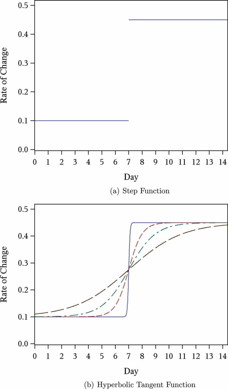
Example plot of rate of change in expected log(CFU) count over time (days).

Then:

which leads to the conventional bilinear regression model for log(CFU) count, namely:

(10)

Here, the parameters α and κ are the intercept and node parameter of the regression curve, respectively, and the slopes λ ₁ and λ ₂ characterize the linear decline on or before the node and after the node , respectively.

Last, we note it is convenient to write the regression model in Equation (10) in terms of the parameters and 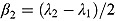, which are, respectively, the average of and half the difference between the two rate constants λ ₁ and λ ₂. Then Equation (10) becomes:

(11)

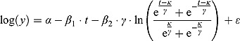
2.2.2. Hyperbolic Tangent Function: Biphasic Regression Model

As has been pointed out by Jindani et al. (2003), the switch from one rate of decline in log(CFU) count to another might be smooth, rather than abrupt as is implied with by the bilinear regression model in Equation (10). In order to model a smooth transition, we can use a monotonic function that interpolates between the early rate of decline, λ ₁, and the late rate of decline, λ ₂. For example, a class of such functions is formed by linear transformations of cumulative distribution functions (Seber and Wild, 1989).

In the following, we model λ(t) using the hyperbolic tangent function:

(12)

The hyperbolic tangent function in Equation (12), shown in Figure 1b, is essentially a smooth version of the step function in Equation (9). For small t, λ(t) tends to λ ₁, i.e. , and similarly, for large t, the function λ(t) tends to λ ₂, i.e. . Furthermore, 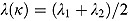, so that κ can be viewed as the “node” of the function λ(t). Last, the parameter γ governs the “smoothness” of the transition from rate λ ₁ to rate λ ₂. With λ(t) as in Equation (12), we obtain as the integral in Equation (8), namely:

Thus, we have the following biphasic nonlinear regression model for log(y):

(13)

Note that, for small t (and small relative to ), the term tends to zero, while the term becomes large. Thus, for small t , declines approximately linearly with slope . Vice versa, for large t, the term becomes large, while the term tends to 0. Thus, for large t, , declines approximately linearly with slope .

In summary, the regression model in Equation (13) is a “smooth” version of the bilinear regression model in Equation (10). (In fact, the regression model in Equation (10) is a special case of the regression model in Equation (13) when .) The parameters and can therefore be interpreted as the “early” and “late” rates of decline, respectively, while the parameter is the intercept of the regression curve. Furthermore, characterizes the “smoothness” of the transition from the early to the terminal decay curve, and is the node parameter. Furthermore, for small t (when ), the variable y (i.e. CFU count on the original scale) is approximated by an exponential function where 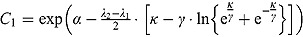and for large t, the variable y is approximated by an exponential function , where 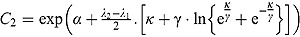. In that sense, the regression model in Equation (13) approximates bi-exponential regression models.

Last, when 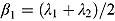and , Equation (13) becomes:

(14)

The regression models in Equation (13) and Equation (14) can be fitted to the log(CFU) count vs. time data of individual patients using maximum likelihood (ML) estimation (similar to conventional “by-patient” regression modeling by Diacon et al. (2012, 2013)). Relevant EBA parameters can accordingly be estimated for each patient based on these model fits.

It should be noted that the regression models in Equation (13) and Equation (14) are similar to models proposed by Bacon and Watts (1971); Griffiths and Miller (1973); Ratkowsky (1983); Grossman et al. (1999), which also have two intersecting line segments as a limiting case; these models comprise parameterizations different to our proposed model.

3. BAYESIAN FIT OF REGRESSION MODELS

3.1. Model 1: Biphasic—Student t Errors and “Default” Wishart Priors

We propose a biphasic hierarchical Bayesian NLME regression model for log(CFU) count vs. time, fitted jointly to the data of all patients from a given trial.

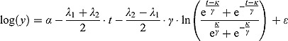
We start by specifying an NLME regression model for the log(CFU) counts. Let be the CFU count for patient in treatment group at time-point , and let be the corresponding measurement time. Then, based on Equation (14), we write the following NLME regression model:

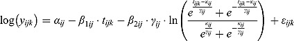(15)

The parameters of the regression model in Equation (15) are analogous to those of the “by-patient” regression model in Equation (14).

The subsections below provide a full specification of the random effects and prior distributions of the regression model in Equation (15).

Random Effects

The vectors 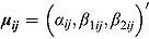of intercept and slope parameters are assumed independent across patients (i.e. independent across indices i and j), with tri-variate normal distributions as follows:

(16)

In Equation (16), 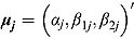are vectors of mean intercepts and slopes, and are the associated covariance matrices, namely:

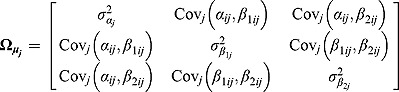Furthermore, the parameters and are assumed to follow truncated normal distributions, independent of each other, and independent of , as follows:

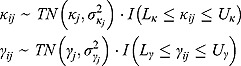(17)

In Equation (17), I(x) denotes an indicator function taking the value 1 if x is true, and 0 otherwise, and , , , and are the prespecified lower bound and upper bound for parameters and , respectively.

Finally, the residuals are assumed to follow independent Student t distributions, independent of , , and , as follows:

(18)

where and v_j are scale parameters and degrees of freedom, respectively, from the corresponding Student t distribution. The specification of the Student t distribution can accommodate heavily tailed residual errors which, in this regard, is more flexible than the normal distribution.

A subset of CFU counts might be reported as zero or “no count” values. Genuine zero counts will typically occur when, for a given patient profile, CFU counts are observed over time to decline to near-zero values, just prior to observing one or more zero counts. Thus, genuine zero counts will typically occur toward the end of a CFU count vs. time profile. When regressing log(CFU) count against time using Equation (15), the log(CFU) counts corresponding to zero count can be specified as a left censored value of 1 (formally, log(y_ijk) < 1) (Rustomjee et al., 2008).

Prior Distributions

In order to complete the Bayesian specification of the NLME regression model described above, proper but vague prior distributions are assigned to all unknown parameters of the NLME regression model.

First, multivariate normal and Wishart prior distributions are specified, respectively, for and in Equation (16), namely:

(19)

(20)

where 0 = (0, 0, 0)′ and I ₃ denotes the 3 × 3 identity matrix. R _j represent 3 × 3 inverse scale matrices.

One challenge is the choice of an appropriate prior distribution for the covariance matrix of the vectors of intercept and slope parameters , i.e. . We used the methodology by Kass and Natarajan (2006), referred to as the “default” Wishart prior, for choosing R_j. This methodology relates to the choice of R_j in the application of generalized linear mixed-effects regression modeling and is derived from the data directly (hence, the resulting posterior distribution does make double use of the data). The inverse scale matrix R_j is derived by selecting the weight which the mean of the “shrinkage” prior, i.e. 0, should contribute toward its posterior (where “shrinkage” represents ). Under the assumption that the node and smoothness parameters are fixed at 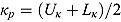and 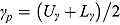, respectively (which are the prior mean for and , respectively (see below)), the regression model with normally distributed errors in Equation (15) reduces to a linear mixed-effects regression model, for which R_j are derived as follows:

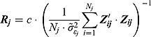(21)

where are the ML estimates of when assuming the regression model is homogeneous across all patients (i.e. disregarding random effects such that , and ). The matrices are defined as follows:

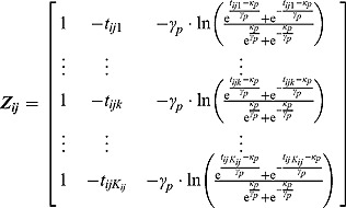We used c = 2.5, causing the mean of the ‘shrinkage” prior, i.e. 0, to have little contribution toward its posterior. The choice of c = 2.5 is equivalent to setting the interval between the lowest and highest possible values for the relative contribution matrix of the mean of the “shrinkage” prior (to its posterior) to 28.6%.

The parameters , , , and (see Equation (17)) are assumed to follow uniform prior distributions, namely , , , and , where , , , are the prespecified lower bound and upper bound for parameters and , respectively.

Finally, the scale parameters and degrees of freedom v_j in Equation (18) are respectively assigned inverse gamma prior distributions, namely , and uniform prior distributions, namely .

For a typical 14-day EBA study, the hyper-parameters of the prior distributions can be chosen as follows: , , (to avoid overfit of the first few and last few observations over time), , (allowing for smooth transition between a few successive data points), , , , and (providing weakly informative prior distributions for the scale parameters and ).

3.2. Model 2: Biphasic—Student t Errors and “Frequentist” Wishart Priors

To assess the sensitivity of results to the choice of R _j, we fitted Model 1 as a linear mixed-effects regression model under the assumption that the node and smoothness parameters (i.e., , , , and ) are fixed at and , respectively. We calculated the “frequentist” estimates for via ML estimation (using the SAS^® procedure PROC NLMIXED) to serve as R_j (SAS Institute Inc., 2008).

3.3. Model 3: Biphasic—Normal Errors and “Default” Wishart Priors

Model 1 can incorporate the assumption that the residual errors follow normal distributions (i.e. instead of Student t distributed residual errors), i.e. , where are the corresponding residual variances following inverse gamma prior distributions, namely .

3.4. Model 4: Biphasic—Normal Errors and “Frequentist” Wishart Priors

The sensitivity of results to the choice of R _j in Model 3 can be assessed using the “frequentist” approach specified for Model 2.

3.5. Model 5: Bilinear—Student t Errors and “Default” Wishart Priors

Based on Equation (11), we can postulate the following bilinear mixed-effects regression model:

(22)

where , and step (x) denotes a function taking the value 0 if , and 1 otherwise. The parameters of the regression model in Equation (22) are analogous to those of the “by-patient” regression model in Equation (11), and the specification of its random effects and prior distributions are similar to those of Model 1.

3.6. Model 6: Bilinear—Normal Errors and “Default” Wishart Priors

Model 5 can incorporate the assumption that the residual errors follow normal distributions (i.e. instead of Student t distributed residual errors).

3.7. Model 7: Monolinear—Student t Errors and “Default” Wishart Priors

The conventional linear mixed-effects regression model can be written as follows:

(23)

The parameters of the regression model in Equation (23) are analogous to those of the “by-patient” regression model in Equation (7), and the specification of its random effects and prior distributions are similar to those of Model 1.

3.8. Model 8: Monolinear—Normal Errors and “Default” Wishart Priors

Model 7 can incorporate the assumption that the residual errors follow normal distributions (i.e. instead of Student t distributed residual errors).

3.9. Posterior Predictive Distributions

The posterior predictive distribution of relevant slope parameters of the Bayesian NLME regression model provides insight into the nature of the EBA of TB treatments; specifically, the posterior predictive distributions of allow one to judge whether treatments are associated with monolinear or biphasic decline of log(CFU) count (depending on whether a future is likely to be close to or substantially different from zero), and whether log(CFU) count initially decreases fast, followed by a slower rate of decrease (if a future is likely to be negative), or vice versa (if a future is likely to be positive). The simulation of the posterior predictive distribution of the future regression slopes (where the subscript f stands for “future patient”) can be implemented in a straightforward manner using the Markov Chain Monte Carlo (MCMC) output of the Gibbs sampling algorithm of the joint posterior distribution of the regression model parameters.

3.10. Model Selection and Model Checking

Alternative NLME regression models can be explored via various Bayesian model selection tools and may be fitted to assess:

• Alternative shapes of the log(CFU) count vs. time profiles, e.g. assuming a linear, bilinear, or biphasic relationship between log(CFU) count and time.

• The sensitivity of results to the choice of prior distributions.

• Alternative distributions for random effects and residuals (error terms).

In order to check our primary model (Model 1; Section 3.1), and to assess the aspects listed above, we fitted the seven additional models (with alternative Bayesian specifications) specified in Section 3.2 through Section 3.8. The fit of each of the models was checked using conditional posterior ordinates (CPOs) and their reciprocals (ICPOs). Some detail is included in the appendix.

Two methods for discriminating between various regression models were considered: The deviance information criterion (DIC) (Spiegelhalter et al., 2002) and Bayes factors (Kass and Raftery, 1995).

3.10.1. Deviance Information Criterion

The DIC is a model adequacy and goodness-of-fit measure and is defined for Model M as follows:

(24)

where is a vector of model parameters, y is an vector of observed data, is the conventional deviance measure (i.e. minus twice the log-likelihood), and are the mean of the posterior distribution of and , respectively, and is the number of “effective” parameters.

The quantity DIC(M) is therefore a measure which takes both goodness of fit and complexity of Model M into account and is more appropriate to assess the predictability of random effects in Model M (Spiegelhalter et al., 2003). The model with the smallest DIC is considered to fit the data more appropriately. However, the DIC measure may be unreliable in cases where is an unreliable estimator of (Ntzoufras, 2009).

3.10.2. Bayes Factors

When comparing Model M ₀ and Model M ₁, based on the posterior probability of each of the models given the data, the Bayes factor in favor of M ₀ is defined as follows:

(25)

where y is an vector of observed data, and and are the marginal likelihoods of y under Model M ₀ and Model M ₁, respectively.

Unlike the DIC, Bayes factors do not explicitly include a term that penalizes model complexity, but rather incorporates the latter in the marginal likelihood of a given model automatically (Ward, 2008). Furthermore, the DIC compares models conditional on their model parameters, whereas the Bayes factors compare models on a marginal basis.

In the case of NLME regression modeling, the marginal likelihoods in Equation (25) need to be approximated. The Laplace–Metropolis approximation, in its general form, for is given by the following expression (Ntzoufras, 2009):

(26)

where and are the mean and standard deviation, respectively, of the posterior distribution of , and is the determinant of the correlation matrix of the posterior distribution of . In mixed-effects models, the calculation of the Laplace–Metropolis marginal likelihood requires that the random effects included in each patient’s likelihood function should be integrated out (Lewis and Raftery, 1997). The five random effects (see Model 1) for each patient were marginalized using the multidimensional integration library R2Cuba of the R project (R Core Team, 2014; Hahn et al., 2013). The Laplace–Metropolis approximation in Equation (26) is based on asymptotic theory of the normal distribution and works well for symmetric posterior distributions of (Ntzoufras, 2009).

3.11. Computational Issues

The OpenBUGS software (Version 3.2.2) is used to implement the MCMC Gibbs sampling algorithm to draw samples from the joint posterior distribution of the model parameters (Gelfand and Smith, 1990; Gilks et al., 1996; Lunn et al., 2009).

Due to the high-dimensional nature of NLME regression models, by-patient parameter estimates, obtained from regression fits (such as Equation (14)) for each patient individually (using SAS^® procedure PROC NLMIXED), were used as starting values for the random effects. The posterior samples were thinned to reduce the autocorrelation among posterior samples. Graphical convergence diagnostics, such as iteration and autocorrelation plots, and the Brooks–Gelman–Rubin statistic (Brooks and Gelman, 1998) for two parallel chains, were used to monitor convergence of posterior samples. Dispersed starting values for the second chain were provided to ensure convergence of the two respective chains. Multidimensional integrals (for calculation of Laplace–Metropolis marginal likelihoods) were calculated using libraries available in the R project (R Core Team, 2014).

4. EMPIRICAL STUDY AND EXAMPLE OF APPLICATION

4.1. Empirical Study

While theoretical considerations may assist in the derivation of a suitable regression model for a certain type of data, the most important requirement for a good regression model is that it should fit the data well. Thus, in deriving a regression model for CFU count, we have started with an empirical study of a large number of log(CFU) count vs. time profiles from four EBA trials. The typical shapes of such profiles, identified in the empirical study, confirm observations made previously by other authors and motivate the theoretical derivation of the biphasic nonlinear regression model proposed in Section 2.2.2.

For the purpose of this empirical study, we have had access to the data from four EBA trials comprising of CFU count vs. time profiles of a total of 291 patients. In all four trials, CFU data were collected over a period of 14 days of treatment. Relevant clinical trial characteristics of clinical trial protocol CL001, CL007, CL010, and NC001 are summarized in Table 1, including the total number of randomized patients, and the number of randomized patients with complete profiles (data up to Day 14).

Table 1 .

Characteristics of clinical trials included in the empirical study

Clinical trial	Scheduled sample days	Treatment group	N	n
CL001	Daily from Day –2 to Day 8;	TMC207 100 mg	15	12
	Day 10, Day 12, Day 14	TMC207 200 mg	15	13
		TMC207 200 mg	15	13
		TMC207 400 mg	15	14
		Rifafour	8	6
		Total	68	58
CL007	Daily from Day –2 to Day 4;	PA-824 200 mg	15	12
	Day 6, Day 8, Day 10, Day 12,	PA-824 600 mg	15	12
	Day 14	PA-824 1000 mg	16	15
		PA-824 1200 mg	15	11
		Rifafour	8	7
		Total	69	57
CL010	Daily from Day –2 to Day 4;	PA-824 50 mg	15	12
	Day 6, Day 8, Day 10, Day 12,	PA-824 100 mg	15	15
	Day 14	PA-824 150 mg	15	14
		PA-824 200 mg	16	14
		Rifafour	8	8
		Total	69	63
NC001	Daily from Day –2 to Day 14	J	15	14
		J -Z	15	12
		J-Pa	15	12
		Pa-Z	15	13
		Pa-Z-M	15	10
		Rifafour	10	8
		Total	85	69
Total		Total	291	247

Notes. Treatment group: J = TMC207, J-Z = TMC207 + Pyrazinamide, J-Pa = TMC207 + PA-824, Pa-Z = PA-824 + Pyrazinamide, Pa-Z-M = PA-824 + Pyrazinamide + Moxifloxacin, Rifafour = Rifafour e-275^®. N = total number of randomized patients. n = number of randomized patients with complete profiles.

The log(CFU) count vs. time profiles of all patients with complete profiles were fitted, separately by patient, using the SAS^® procedure NLMIXED. Note that we used only patients with complete data profiles since the primary purpose of the empirical study was to judge the adequacy of the proposed biphasic model specifically when fitted to 14-day CFU count vs. time profiles; naturally, when data profiles are (substantially) shorter than 14 days (e.g. due to a patient dropping out of a trial early), a simple monolinear model will often be adequate.

Plots of the data together with by-patient fits of the biphasic regression model are included as Figure A.1 through Figure A.21 in the supplementary material. The residuals were assumed to follow independent and identically distributed normal distributions, and the lower and upper bounds of κ and γ were respectively set to , , , and . Studying the data profiles, we noted the following (see Table 4.2):

Table 2 .

“By-patient” regression model parameter estimates for empirical study

			Mean (range)
Clinical trial	Treatment group	n	κ	λ1	λ2	nL	nB	nBFS	nBSF	nBI	nBM
CL00l	TMC207 100 mg	12	5.8 (2.0–11.0)	0.082 (−0.276–0.782)	0.062 (−0.093–0.303)	2	10	5	5	9	1
	TMC207 200 mg	13	6.6 (2.0–10.8)	−0.054 (−0.385–0.099)	0.167 (−0.006–0.497)	1	12	1	11	11	1
	TMC207 300 mg	13	6.3 (2.0–11.0)	0.058 (−0.070–0.446)	0.122 (−0.158–0.388)	3	10	3	7	9	1
	TMC207 400 mg	14	6.8 (2.0–11.0)	0.074 (−0.280–0.289)	0.141 (−0.066–0.463)	9	5	1	4	5	0
	Rifafour	6	3.8 (2.0–11.0)	0.283 (−0.278–0.534)	−0.110 (−0.957–0.167)	0	6	5	1	5	1
	Total	58	6.1 (2.0–11.0)	0.065 (−0.385–0.782)	0.100 (−0.957–0.497)	15	43	15	28	39	4
CL007	PA-824 200 mg	12	6.5 (2.0–11.0)	0.202 (−0.565–0.618)	−0.019 (−0.348–0.226)	0	12	9	3	11	1
	PA-824 600 mg	12	6.9 (2.8–11.0)	0.135 (−0.233–0.326)	0.045 (−0.271–0.269)	1	11	7	4	11	0
	PA-824 1000 mg	15	6.7 (2.0–11.0)	0.111 (−0.541–0.490)	0.052 (−0.231–0.539)	1	14	8	6	11	3
	PA-824 1200 mg	11	6.9 (2.0–11.0)	0.065 (−0.559–0.413)	0.056 (−0.529–0.722)	2	9	6	3	8	1
	Rifafour	7	5.0 (2.0–8.1)	0.378 (0.192–0.629)	−0.005 (−0.129–0.124)	0	7	7	0	6	1
	Total	57	6.5 (2.0–11.0)	0.159 (−0.565–0.629)	0.029 (−0.529–0.722)	4	53	37	16	47	6
CL010	PA-824 50 mg	12	6.1 (2.0–11.0)	0.141 (−0.040–0.525)	0.045 (−0.168–0.366)	3	9	7	2	9	0
	PA-824 100 mg	15	6.1 (2.0–11.0)	0.084 (−1.032–0.629)	0.049 (−0.131–0.244)	2	13	8	5	10	3
	PA-824 150 mg	14	6.5 (2.0–11.0)	0.022 (−0.439–0.302)	0.024 (−0.287–0.284)	2	12	8	4	12	0
	PA-824 200 mg	14	5.8 (2.0–10.0)	0.193 (−0.046–0.648)	0.108 (−0.022–0.419)	3	11	8	3	10	1
	Rifafour	8	6.7 (2.0–11.0)	0.370 (0.060–1.144)	0.166 (−0.033–0.397)	0	8	5	3	7	1
	Total	63	6.2 (2.0–11.0)	0.141 (−1.032–1.144)	0.070 (−0.287–0.419)	10	53	36	17	48	5
NC001	J	14	6.9 (2.2–11.0)	−0.014 (−0.433–0.188)	0.216 (−0.099–0.718)	2	12	2	10	10	2
	J-Ζ	12	5.8 (2.0–11.0)	0.046 (−0.227–0.280)	0.156 (0.042–0.322)	4	8	2	6	7	1
	J-Pa	12	6.3 (2.0–11.0)	0.081 (−0.151–0.321)	0.049 (−0.176–0.155)	1	11	6	5	10	1
	Pa-Z	13	8.0 (2.0–11.0)	0.189 (−0.663–1.122)	0.091 (−0.131–0.451)	2	11	8	3	10	1
	Pa-Z-M	10	5.7 (2.0–11.0)	0.378 (0.080–0.721)	0.060 (−0.229–0.194)	1	9	9	0	7	2
	Rifafour	8	7.3 (2.0–11.0)	0.161 (0.025–0.273)	0.179 (−0.041–0.475)	1	7	3	4	6	1
	Total	69	6.7 (2.0–11.0)	0.128 (−0.663–1.122)	0.126 (−0.229–0.718)	11	58	30	28	50	8
Total	Total	247	6.4 (2.0–11.0)	0.124 (−1.032–1.144)	0.083 (−0.957–0.722)	40	207	118	89	184	23

Notes. Treatment group: J = TMC207, J-Z = TMC207 + Pyrazinamide, J-Pa = TMC207 + PA-824, Pa-Z = PA-824 + Pyrazinamide, Pa-Z-M = PA-824 + Pyrazinamide + Moxifloxacin, Rifafour = Rifafour e-275^®. n = number of randomized patients with complete profiles. n _L = number of linearly decreasing profiles . n _B = number of biphasic profiles . n _BFS = number of biphasic profiles in which the initial rate of decrease is fast, followed by slower rate of decrease . n _BSF = number of biphasic profiles in which initial rate of decrease is slow, followed by a faster rate of decrease . n _BI = number of bilinear profiles with abrupt transition between the two rates of decrease . n _BM = number of biphasic profiles with smooth transition between the two rates of decrease .

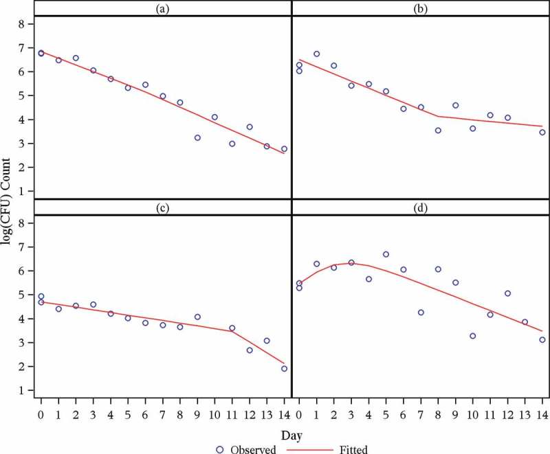
1. Over the profile period of 14 days, the log(CFU) count vs. time profiles seem either linear (for the minority of patients: 40 out of 247) or biphasic (for the majority of patients: 207 out of 247). For an example of a (near) linear profile, see Figure 1a; examples of clearly biphasic profiles are given in Figures 1b through Figure 1d.

2. The rate of decline in log(CFU) count during the initial phase is greater than during the terminal phase for the majority of biphasic profiles (e.g. Figure 1b); the rate of decline in log(CFU) count during the initial phase is smaller than during the terminal phase for the minority of biphasic profiles (e.g. Figure 1c).

3. The transition from the first to the second phase is smooth for a minority of biphasic profiles (e.g. Figure 1d); a bilinear regression model seems adequate for the majority of biphasic profiles (e.g. Figure 1b and Figure 1c).

4. The average rate of decline in log(CFU) count during the initial phase is for some treatment regimens greater than during the terminal phase. However, for one of the newer compounds under investigation, bedaquiline (TMC207), and for some treatment regimens containing TMC207 in combination with other drugs, the average rate of decline in log(CFU) count during the initial phase is smaller than during the terminal phase.

5. Whatever the respective average rates of decline in log(CFU) count for a given treatment regimen, rates of decline both during the initial and late phases exhibit appreciable interindividual variability; for individual patients, the rate of decline in log(CFU) count during the initial phase might be smaller than during the late phase, even though the respective average rates for the treatment regimen in question might exhibit the reverse relationship.

6. The time-point (node) at which the initial rate of decline changes to the terminal rate of decline exhibits appreciable individual variability (possibly as a result of little information for the estimation of the node parameter).

Figure 2 .

Fitted log(CFU) counts vs. time for empirical study.

Observations from the empirical study suggest the following:

• Bilinear regression models seem adequate for the log(CFU) count vs. time profiles of many patients, but certainly not for all, since a substantial minority of profiles exhibit a smooth transition between phases. Whatever the case may be, it is preferable to fit a regression model that allows for a smooth transition between phases, thereby allowing one to judge the adequacy of the bilinear regression model.

• Bilinear regression models need to accommodate individual variation in the node and should estimate the node parameter from the data, rather than determining it through visual inspection.

• Bi-exponential regression models are not adequate for treatments (and individual profiles) which are associated with terminal rates of decline that are faster than initial rates of decline.

• The log(CFU) count vs. time profiles suggest that the residual variance is constant over the range of fitted values, i.e., the logarithm is effective as variance stabilizing transformation.

On the whole, a visual inspection of the model fits suggests that the proposed regression model generally fits the data well (see Figure A.1 through Figure A.21 in the supplementary material).

4.2. Example of Application

We fitted the Bayesian NLME regression model in Equation (15) (Model 1) to the data of the NC001 trial (see Table 2) (Diacon et al., 2012) and compared its fit with that of the alternative regression models (Model 2 through Model 8).

Model Selection

Model comparison statistics for the various Bayesian NLME regression models fitted are provided in Table 3. The model comparison statistics appear to be sensitive to the choice of the hyper-parameters of the Wishart prior distributions (“default” vs. “frequentist”): This, however, is a well-known drawback (Lindley, 1993) with the use of Bayes factors. The DIC favors bilinear models slightly over biphasic models, followed by linear models. The marginal likelihood (Bayes factor) criterion favors linear models, followed by biphasic and bilinear models. Both the DIC and marginal likelihood (Bayes factor) criteria favor models with Student t distributed errors over those with normally distributed errors.

Table 3 .

Comparison of Bayesian NLME regression models

	DIC					% ICPO < x
Model				DIC(M)
Model 1	1335.00	1144.00	191.00	1526.002	−1365.664	97.57	98.87	99.11
Model 2	1360.00	1158.00	202.70	1563.003	−1336.713	97.73	98.95	99.19
Model 3	1454.00	1273.00	180.70	1635.005	−1382.127	97.98	98.62	98.95
Model 4	1476.00	1282.00	194.40	1671.006	−1367.235	97.73	98.70	99.03
Model 5	1324.00	1127.00	197.20	1521.001	−1376.756	97.57	98.87	99.19
Model 6	1445.00	1257.00	187.40	1632.004	−1408.108	97.89	98.54	98.95
Model 7	1565.00	1398.00	167.50	1733.007	−1236.991	98.54	99.11	99.19
Model 8	1644.00	1481.00	162.50	1806.008	−1262.322	98.54	98.95	99.11

Notes. CPO: conditional posterior ordinate; ICPO: reciprocal of CPO; DIC: deviance information criterion. Model 1: biphasic: Student t errors and “default” Wishart priors. Model 2: biphasic: Student t errors and “frequentist” Wishart priors. Model 3: biphasic: normal errors and “default” Wishart priors. Model 4: biphasic: normal errors and “frequentist” Wishart priors. Model 5: bilinear: Student t errors and “default” Wishart priors. Model 6: bilinear: normal errors and “default” Wishart priors. Model 7: monolinear: Student t errors and “default” Wishart priors. Model 8: monolinear: normal errors and “default” Wishart priors. Superscripts indicate the ranking of model comparison statistics from least favored (1) to most favored (8).

The ICPOs suggest all models fit the data reasonably well.

Early Bactericidal Activity of Study Treatments

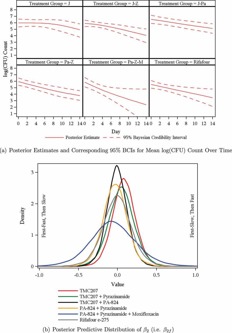
Posterior estimates and corresponding 95% Bayesian credibility intervals (BCIs) for the mean EBA of Model 1, including pairwise comparisons vs. Rifafour, are presented in Table 4. Posterior estimates and corresponding 95% BCIs for the mean regression model parameters of Model 1 are included as supplementary material to this article (Table B.1). Mean EBA(0–14) was significantly different from 0 for each treatment regimen. Treatment with Pa-Z-M had the highest bactericidal activity both over the whole 14-day treatment period and over the time intervals Day 0 to Day 2 and Day 2 to Day 14. These results can be compared to those published by Diacon et al. (2012).

Table 4 .

Model 1—Inferential statistics for mean EBA

			Mean		Mean vs. rifafour
Parameter	Treatment	n	Estimate	95% BCI	Estimate	95% BCI
EBA(0–14)	J (N=15)	15	0.074	[0.010; 0.145]	−0.073	[−0.185; 0.042]
	J-Z (N=15)	15	0.133	[0.065; 0.204]	−0.013	[−0.128; 0.101]
	J-Pa (N = 15)	15	0.101	[0.056; 0.146]	−0.045	[−0.147; 0.055]
	Pa-Z (N = 15)	15	0.154	[0.100; 0.207]	0.007	[−0.098; 0.113]
	Pa-Z-M (N = 15)	15	0.248	[0.087; 0.430]	0.102	[−0.082; 0.304]
	Rifafour (N = 10)	10	0.146	[0.055; 0.238]
EBA(0–2)	J (N = 15)	15	−0.002	[−0.086; 0.084]	−0.156	[−0.316; 0.000]
	J-Z (N = 15)	15	0.069	[−0.038; 0.170]	−0.085	[−0.254; 0.081]
	J-Pa (N = 15)	15	0.105	[0.019; 0.187]	−0.049	[−0.210; 0.105]
	Pa-Z (N = 15)	15	0.179	[0.079; 0.277]	0.025	[−0.142; 0.187]
	Pa-Z-M (N = 15)	15	0.313	[0.164; 0.460]	0.159	[−0.040; 0.355]
	Rifafour (N = 10)	10	0.154	[0.021; 0.290]
EBA(2 -14)	J (N = 15)	15	0.086	[0.019; 0.170]	−0.059	[−0.185; 0.075]
	J-Z (N = 15)	15	0.144	[0.066; 0.229]	−0.001	[−0.132; 0.133]
	J-Pa (N = 15)	15	0.100	[0.053; 0.148]	−0.044	[−0.160; 0.072]
	Pa-Z (N = 15)	15	0.149	[0.093; 0.203]	0.004	[−0.114; 0.124]
	Pa-Z-M (N = 15)	15	0.238	[0.046; 0.455]	0.093	[−0.124; 0.330]
	Rifafour (N = 10)	10	0.145	[0.037; 0.251]

Notes. Treatment group: J = TMC207, J-Z = TMC207 + Pyrazinamide, J-Pa = TMC207 + PA-824, Pa-Z = PA-824 + Pyrazinamide, Pa-Z-M = PA-824 + Pyrazinamide + Moxifloxacin, Rifafour = Rifafour e-275^®. EBA: early bactericidal activity over Day to Day ; BCI: Bayesian credibility interval; n = number of patients in each category.

Posterior estimates and corresponding 95% BCIs for the mean log(CFU) count vs. time profiles of the six treatment regimens are presented for Model 1 in Figure 2a and for Model 2 through Model 8 as supplementary material to this article (Figure B.1 to Figure B.7, respectively). The posterior estimates and corresponding 95% BCIs for the mean log(CFU) count vs. time profiles were similar for Model 1 to Model 8.

Figure 3 .

Model 1—Mean log(CFU) count and posterior predictive distributions.

The posterior predictive distributions of the (i.e., ) based on Model 1 are presented in Figure 2b for each treatment group. The estimates for the mean and per treatment group suggest that the initial rate of decrease in CFU count for some treatment groups containing TMC207 (i.e. J and J-Z) is slow, followed by a faster rate, and vice versa for the treatment groups not containing TMC207 (Pa-Z and Pa-Z-M, and Rifafour). The decrease in mean log(CFU) count of J-Pa is effectively linear over time. The estimates for the mean per treatment group suggest that the mean log(CFU) count switches from one rate of decrease to another smoothly.

5. DISCUSSION

EBA trials of TB treatments assess the decline, during the first few days to weeks of treatment, in CFU count of Mycobacterium tuberculosis in the sputum of patients with smear-microscopy-positive pulmonary TB (Diacon et al., 2012). EBA trials are a mainstay in the early clinical development of TB treatment regimens and thus are frequently performed.

The research reported in this article was motivated by the need for a general and flexible regression model for CFU count vs. time data. Such data have conventionally been modeled using linear, bilinear, or bi-exponential regression. Linear regression, while potentially appropriate for some individual profiles, is not generally adequate since many data profiles are clearly biphasic, at least for treatment and observation periods longer than 2 to 7 days. Both bilinear and bi-exponential models seem adequate for many individual profiles, but the former do not allow for a smooth transition between the initial and terminal phases of decline of CFU counts, while the latter cannot account for drugs and individual profiles which are associated with terminal rates of decline that are faster than initial rates of decline. Such terminal rates of decline have been described only recently.

In this article, we have proposed a biphasic nonlinear regression model for CFU data that comprises linear and bilinear regression models as special cases and is more flexible than bi-exponential regression models. An extensive empirical study of a large number of CFU count vs. time profiles from a database of four EBA trials suggests that the proposed model fits well virtually all individual profiles. We have implemented the model as a Bayesian NLME regression model, fitted jointly to the data of all patients from a trial. One advantage of the Bayesian implementation of the model is that for patients with incomplete and sparse profiles (due to missing data), it is generally plausible as “strength is borrowed” from the remainder of the data, which manifests as random-effects estimates are shrunken toward the overall mean.

Statistical inference about the mean EBA of TB treatments is based on the Bayesian NLME regression model. The posterior predictive distribution of relevant slope parameters of the Bayesian NLME regression model provides insight into the nature of the EBA of TB treatments; specifically, the posterior predictive distribution of slope parameters allows one to judge whether treatments are associated with monolinear or bilinear decline of log(CFU) count, and whether log(CFU) count initially decreases fast, followed by a slower rate of decrease, or vice versa. In this regard, our analysis of data from the NC001 trial confirms that TMC207, somewhat unusually among anti-TB treatments, is a drug associated with a terminal rate of decline in CFU count that is faster than the initial rate of decline.

Our primary Bayesian implementation of the regression model was based on the Student t error distribution and the so-called “default” Wishart prior for the covariance matrix of the random intercept and slope parameters. However, the fit of alternative specifications of error and prior distributions was also explored. It seems that the Student t distribution, which allows for heavier tails than the normal distribution, better accommodates occasional outliers seen in the data. The DICs favor bilinear models slightly over biphasic models, followed by linear models, whereas the Bayes factors favor linear models, followed by biphasic and bilinear models. Given the different verdicts, it should be noted that the DIC compares models conditional on their model parameters (for which their random effects are likely to enhance model fit), whereas the Bayes factors compare models on a marginal basis. With our analysis, the Bayes factors prefer the simplest model (i.e. linear) over the more refined models (i.e. biphasic and bilinear), whereas the DICs prefer the latter. Note that the linear model cannot establish to which extent the bactericidal activity between initial and later phases of treatment differs, and investigation of this difference is a crucial aspect of EBA studies.

In summary, the biphasic model (Model 1) proposed here empirically fits well all individual data profiles studied and, according to the marginal likelihood (Bayes factor) criterion, is favored over the bilinear model. Furthermore, the biphasic model allows one to quantify differences in early and late rates of decline of CFU counts, which is of some importance in characterizing the mode of action of anti-TB treatments.

Supplementary Material

Supplemental data for this article can be accessed on the publisher’s website.

APPENDIX

Model checking can include the assessment of the predictive performance of the regression model using the posterior predictive distribution of replicated data . The goodness of fit between replicated and observed data can be assessed accordingly (Ntzoufras, 2009).

The posterior predictive distribution of is given by the following expression:

(27)

where , y, and represent a , , and vector of replicated and observed data, and model parameters, respectively.

The aforementioned approach has been criticized because of its double use of the data, and as a result, Geisser and Eddy (1979) proposed the use of the leave-one-out cross-validation predictive distribution instead, namely:

(28)

where represents the vector y with the ith observation (i.e. y_i) omitted.

The quantity in Equation (28) is also known as the CPO and can be estimated by the following:

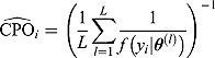(29)

where represents the vector of posterior MCMC samples from θ at iteration l. The estimate can be interpreted as the harmonic mean of the probability distribution of y_i for each , where following the simulation burn-in period.

A large number of small estimates would indicate a poor fit of the candidate model. Such estimates can also be used to identify possible outliers in the data. Conversely, the reciprocal of , or , can also be used to assess model fit. Estimates of and highlight possible or extreme outliers in the data, respectively (Ntzoufras, 2009).

REFERENCES

- Bacon D. W., Watts D. G. Estimating the transition between two intersecting straight lines. Biometrika. 1971;58:525–534. [Google Scholar]
- Botha F. J. H., Sirgel F. A., Parkin D. P., Van De Wal B. W., Donald P. R., Mitchison D. A. Early bactericidal activity of ethambutol, pyrazinamide and the fixed combination of isoniazid, rifampicin and pyrazinamide (Rifater) in patients with pulmonary tuberculosis. South African Medical Journal. 1996;86(2):155–158. [PubMed] [Google Scholar]
- Brindle R., Odhiambo J. A., Mitchison D. A. Serial counts for Mycobacterium tuberculosis in sputum as surrogate markers for the sterilising activity of rifampicin and pyrazinamide in treating pulmonary tuberculosis. BMC Pulmonary Medicine. 2001;1(1):2. doi: 10.1186/1471-2466-1-2. [DOI] [PMC free article] [PubMed] [Google Scholar]
- Brooks S. P., Gelman A. General methods for monitoring convergence of iterative simulations. Journal of Computational and Graphical Statistics. 1998;7:434–455. [Google Scholar]
- Davies G. R., Brindle R., Khoo S. H., Aarons L. J. Use of nonlinear mixed-effects analysis for improved precision of early pharmacodynamic measures in tuberculosis treatment. Antimicrobial Agents and Chemotherapy. 2006a;50:3154–3156. doi: 10.1128/AAC.00774-05. [DOI] [PMC free article] [PubMed] [Google Scholar]
- Davies G. R., Khoo S. H., Aarons L. J. Optimal sampling strategies for early pharmacodynamic measures in tuberculosis. Journal of Antimicrobial Chemotherapy. 2006b;58:594–600. doi: 10.1093/jac/dkl272. [DOI] [PubMed] [Google Scholar]
- Diacon A. H., Dawson R., Von Groote-Bidlingmaier F., Symons G., Venter A., Donald P. R., Conradie A., Erondu N., Ginsberg A. M., Egizi E., Winter H., Becker P., Mendel C. M. Randomized dose-ranging study of the 14-day early bactericidal activity of bedaquiline (TMC207) in patients with sputum microscopy smear-positive pulmonary tuberculosis. Antimicrobial Agents and Chemotherapy. 2013;57(5):2199–2203. doi: 10.1128/AAC.02243-12. [DOI] [PMC free article] [PubMed] [Google Scholar]
- Diacon A. H., Dawson R., Von Groote-Bidlingmaier F., Symons G., Venter A., Donald P. R., Van Niekerk C., Everitt D., Winter H., Becker P., Mendel C. M., Spigelmin M. K. 14-Day bactericidal activity of PA-824, bedaquiline, pyrazinamide, and moxifloxacin combinations: A randomized trial. The Lancet. 2012;380:986–993. doi: 10.1016/S0140-6736(12)61080-0. [DOI] [PubMed] [Google Scholar]
- Dietze R., Hadad D. J., McGee B., Molino L. P. D., Maciel E. L. N., Peloquin C. A., Johnson D. F., Debanne S. M., Eisenach K., Boom W. H., Palaci M., Johnson J. L. Early and extended early bactericidal activity of linezolid in pulmonary tuberculosis. American Journal of Respiratory and Critical Care Medicine. 2008;178:1180–1185. doi: 10.1164/rccm.200806-892OC. [DOI] [PMC free article] [PubMed] [Google Scholar]
- Donald P. R., Diacon A. H. The early bactericidal activity of anti-tuberculosis drugs: A literature review. Tuberculosis. 2008;88(Suppl 1):S75–S83. doi: 10.1016/S1472-9792(08)70038-6. [DOI] [PubMed] [Google Scholar]
- Geisser S., Eddy W. F. A predictive approach to model selection. Journal of the American Statistical Association. 1979;74:153–160. [Google Scholar]
- Gelfand A. E., Smith A. F. M. Sampling-based approaches to calculating marginal densities. Journal of the American Statistical Association. 1990;85:398–409. [Google Scholar]
- Gilks W. R., Richardson S., Spiegelhalter D. J. Markov Chain Monte Carlo in Practice. London, UK: Chapman and Hall; 1996. [Google Scholar]
- Gillespie S. H., Gosling R. D., Charalambous B. M. A reiterative method for calculating the early bactericidal activity of antituberculosis drugs. American Journal of Respiratory and Critical Care Medicine. 2002;166:31–35. doi: 10.1164/rccm.2112077. [DOI] [PubMed] [Google Scholar]
- Griffiths D. A., Miller A. J. Hyperbolic regression - A model based on two-phase piecewise linear regression with a smooth transition between regimens. Communications in Statistics. 1973;2:561–569. [Google Scholar]
- Grossman M., Hartz S. M., Koops W. J. Persistency of lactation yield: A novel approach. Journal of Dairy Science. 1999;82(10):2192–2197. doi: 10.3168/jds.S0022-0302(99)75464-0. [DOI] [PubMed] [Google Scholar]
- 2013 http://CRAN.R-project.org/package=R2Cuba Hahn, H., Bouvier, A., Kiu, K. R2Cuba: Multidimensional Numerical Integration. R package Version 1.0-11. URL.
- Jindani A., Doré C. J., Mitchison D. A. Bactericidal and sterilizing activities of antituberculosis drugs during the first 14 days. American Journal of Respiratory and Critical Care Medicine. 2003;167:1348–1354. doi: 10.1164/rccm.200210-1125OC. [DOI] [PubMed] [Google Scholar]
- Kass R. E., Natarajan R. A default conjugate prior for variance components in generalized linear mixed models (comments on article by Browne and Draper) Bayesian Analysis. 2006;1(3):535–542. [Google Scholar]
- Kass R. E., Raftery A. E. Bayes factors. Journal of the American Statistical Association. 1995;90:773–795. [Google Scholar]
- Lewis S. M., Raftery A. E. Estimating Bayes factor via posterior simulation with Laplace–Metropolis estimator. Journal of the American Statistical Association. 1997;92:648–655. [Google Scholar]
- Lindley D. V. On presentation of evidence. Mathematical Scientist. 1993;18:60–63. [Google Scholar]
- Lunn D. J., Spiegelhalter D. J., Thomas A., Best N. G. The BUGS project: Evolution, critique and future directions. Statistics in Medicine. 2009;28:3049–3067. doi: 10.1002/sim.3680. [DOI] [PubMed] [Google Scholar]
- Mitchison D. A. Clinical development of anti-tuberculosis drugs. Journal of Antimicrobial Chemotherapy. 2006;58:494–495. doi: 10.1093/jac/dkl260. [DOI] [PubMed] [Google Scholar]
- Mitchison D. A., Davies G. R. Assessment of the efficacy of new anti-tuberculosis drugs. The Open Infectious Diseases Journal. 2008;2:59–76. doi: 10.2174/1874279300802010059. [DOI] [PMC free article] [PubMed] [Google Scholar]
- Mitchison D. A., Sturm W. A. The measurement of early bactericidal activity. In: Malin A., McAdam K. P. W. J., editors. Bailliere’s Clinical Infectious Diseases: Mycobacterial Diseases Part II. London: Bailliere Tindall; 1997. pp. 185–206. [Google Scholar]
- Ntzoufras I. Bayesian Modeling Using WinBUGS. Hoboken, New Jersey: John Wiley & Sons, Inc; 2009. [Google Scholar]
- Phillips P., Fielding K. Surrogate markers for poor outcome to treatment for tuberculosis: Results from extensive multi-trial analysis. The International Journal of Tuberculosis and Lung Disease. 2008;12:S146–S147. [Google Scholar]
- 2014 http://www.R-project.org/ R Core Team. R: A Language and Environment for Statistical Computing, R Foundation for Statistical Computing, Vienna, Austria. URL.
- Ratkowsky D. A. Nonlinear Regression Modeling: A Unified Practical Approach. New York: Marcel Dekker; 1983. [Google Scholar]
- Rustomjee R., Lienhardt C., Kanyok T., Davies G. R., Levin J., Mthiyane T., Reddy C., Sturm A. W., Sirgel F. A., Allen J., Coleman D. J., Fourie B., A., M. D., the Gatifloxacin for TB (OFLOTUB) Study Team A Phase II study of the sterilising activities of ofloxacin, gatifloxacin and moxifloxacin in pulmonary tuberculosis. The International Journal of Tuberculosis and Lung Disease. 2008;12(2):128–138. [PubMed] [Google Scholar]
- SAS Institute Inc. SAS/STATR 9.2 User’s Guide. Cary, North Carolina: Author; 2008. [Google Scholar]
- Seber G. A. F., Wild C. J. Nonlinear Regression. New York: Wiley Press; 1989. [Google Scholar]
- Spiegelhalter D. J., Best N. G., Carlin B. P., Van Der Linde A. Bayesian measures of model complexity and fit (with discussion) Journal of the Royal Statistical Society. 2002;64:583–640. [Google Scholar]
- 2003 http://www.politicalbubbles.org/bayes_beach/manual14.pdf Spiegelhalter, D. J., Thomas, A., Best, N. G., Lunn, D. Win-BUGS User Manual, Version 1.4. URL.
- O’Brien R. J. Studies of the early bactericidal activity of new drugs for tuberculosis: A help or a hindrance to antituberculosis drug development? American Journal of Respiratory and Critical Care Medicine. 2002;166:3–4. doi: 10.1164/rccm.2205007. [DOI] [PubMed] [Google Scholar]
- Wallis R. S., Doherty T. M., Onyebujoh P., Vahedi M., Laang H., Olesen O., Parida S., Zumla A. Biomarkers for tuberculosis disease activity, cure, and relapse. The Lancet Infectious Diseases. 2009;9:162–172. doi: 10.1016/S1473-3099(09)70042-8. [DOI] [PubMed] [Google Scholar]
- Ward E. J. A review and comparison of four commonly used Bayesian and maximum likelihood model selection tools. Ecological Modelling. 2008;211:1–10. [Google Scholar]
- 2011 http://www.plosone.org/article/info:doi/10.1371/journal.pone.0020343 Yang, Y., Li, X., Zhou, F., Jin, Q., Gao, L. Prevalence of drug-resistant tuberculosis in mainland china: Systematic review and meta-analysis. PLoS ONE 6(6):e20343. URL.
Associated Data
This section collects any data citations, data availability statements, or supplementary materials included in this article.