Atomic Bomb Survivors Life-Span Study

Abstract

The atomic bomb survivors life-span study (LSS) is often claimed to support the linear no-threshold hypothesis (LNTH) of radiation carcinogenesis. This paper shows that this claim is baseless. The LSS data are equally or better described by an s-shaped dependence on radiation exposure with a threshold of about 0.3 Sievert (Sv) and saturation level at about 1.5 Sv. A Monte-Carlo simulation of possible LSS outcomes demonstrates that, given the weak statistical power, LSS cannot provide support for LNTH. Even if the LNTH is used at low dose and dose rates, its estimation of excess cancer mortality should be communicated as 2.5% per Sv, i.e., an increase of cancer mortality from about 20% spontaneous mortality to about 22.5% per Sv, which is about half of the usually cited value. The impact of the “neutron discrepancy problem” – the apparent difference between the calculated and measured values of neutron flux in Hiroshima – was studied and found to be marginal. Major revision of the radiation risk assessment paradigm is required.

INTRODUCTION

The atomic bomb survivors of Hiroshima and Nagasaki are subject to follow-up study for their remaining lives, starting from 1950. Results of this Life-Span Study (LSS), being conducted by the Radiation Effects Research Foundation (RERF), are used by international advisory and standard-setting bodies in establishing recommendations for radiation protection (UNSCEAR 2000). It has been even stated that “the LSS cohort of Atomic-bomb survivors serves as the single most important source of data for evaluating risks of … radiation” (NRC 2006; p. 141). As such, the LSS became crucial in justifying the linear no-threshold hypothesis (LNTH) of radiation-induced cancers.

The LNTH is based on the assumption that each ionizing radiation dose increment, no matter how small, increases the cancer risk. The excess risk is assumed to increase linearly as total dose increases, with an adjustment to the slope of the dose-response relationship for the reduced risk at low dose rates. Typically, the slope is scaled down by a factor of 1.5–2.0 for low dose rates in comparison to the acute exposures received by the A-bomb survivors. The LNTH is employed for cancer risk assessment (UNSCEAR 2013, NRC 2006) and is also relied on by the regulatory organizations becoming the basis for the radiation safety regulations. These are designed to minimize the hypothetical risks of cancer deaths by keeping radiation exposures “as low as reasonably achievable” (ALARA). Moreover, the notion that radiation, in any amount, increases the risk of cancer is widely accepted by the general public. However, the scientific validity of this hypothesis has never been established and has been seriously questioned and debated for many decades (Taylor 1980; Jaworowski 1999; Feinendegen et al. 2013). On the contrary, numerous studies (experimental, epidemiological, and ecological) have shown that low doses of ionizing radiation are beneficial to health (Feinendegen et al. 2004; Jaworowski 2008; Tubiana et al. 2009). The absence of scientific consensus has always been acknowledged by official bodies, including the US Congress Office of Technology Assessment (OTA 1979).

The present radiation protection regulations impose excessive costs to the society, effectively leading to loss, rather than saving, of life. For example, costs of radiation protection are about 5000 times higher than the cost of protection of workers from all other and much more probable events. At Chernobyl and Fukushima, compulsory relocation (inspired by ALARA and the LNTH predictions) led to social destruction, which caused significant emotional/psychological problems and a considerable number of premature deaths. These and other aspects of the LNTH human costs are dealt elsewhere (Socol et al. 2014).

Taking into account (a) the dominant role that the LSS findings played in setting the present no-threshold radiation risk assessment paradigm (and consequently – radiation protection standards), (b) the vast scientific evidence supporting effective thresholds (safe dose levels) for radiation carcinogenesis and (c) the high costs, including human costs, of radiation protection in its present form, the LSS results should be subjected to serious scientific scrutiny. Doss (2012) and Sasaki et al. (2014) challenged the RERF conclusion that the LSS results support the LNTH (Ozasa et al. 2012). However, the above authors employed data processing methods that could better suit more precise data. Our goal was to analyze the LSS data using direct method enabling transparent comparison with RERF results.

METHOD

The data of the atomic bomb survivors life-span study (LSS) are available at the Radiation Effects Research Foundation (RERF) website: www.rerf.or.jp. The LSS cohort consists of 86,661 members. RERF does not provide individual data vectors for each cohort member for privacy and other concerns. Instead, the Foundation provides data for 53,782 groups of members. The members are grouped according to city, sex, age at exposure (15 categories: 0-5, 5-10, …, 65-70 and 70+), time period (11 categories: 1950-1955, 1956-1960, …, 2001-2003), age at death (21 categories: 0-5, 5-10, …, 95-100 and 100+), weighted colon dose (22 categories: 0-5, 5-20, 20-40 mSv, etc) and more. For each group, RERF provides 51 variables, including a count of subjects entering the study, mean organ doses and disease death counts for each cause of death. Only a few were used in this reanalysis, like total number entering the study, colon and breast doses, total deaths and solid cancer deaths.

Let us define mortality ratio (MR) for a certain cause of death as the ratio of the number of these deaths during the whole LSS period 1950-2003 to the number of persons entering LSS. (In this paper, “mortality” is often used for MR, for simplicity). For example, 50,620 LSS participants died from all causes during the reported period 1950-2003, so MR(all causes) = 50,620 / 86,661 ≈ 0.58; the number of deaths from all types of solid cancer is 10,929, so MR(solid cancers)= 10,929 / 86,661≈ 0.13.

We define the excess mortality ratio (EMR) as

$$EMR\hspace{0.17em}=\hspace{0.17em}[\hspace{0.17em}MR\hspace{0.17em}-\hspace{0.17em}M{R}_{\exp ected}]\hspace{0.17em}/\hspace{0.17em}M{R}_{\exp ected}\hspace{0.17em}\hspace{0.17em}\hspace{0.17em}\hspace{0.17em}\hspace{0.17em}$$ 1a

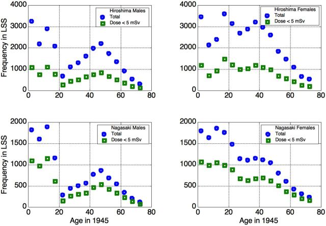
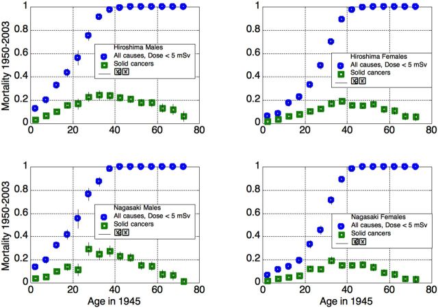
where MR_expected is the expected mortality ratio. For all solid cancers, MR_expected was calculated as follows. First, the age distributions were determined for each of the 22(dose categories) × 2(city) × 2(sex) groups. Then the lowest-dose (below 5 mSv) survivors were designated as a reference (control) group (Fig.1). Next, MR₀(solid cancers) was determined as a function of age at exposure for each city and sex (Fig.2). Then, the initial number of survivors N_ijk(D), within each group sharing city (index i), sex (j), age at exposure (k) and dose category (D), – was multiplied by MR₀^ijk corresponding to the same city, sex and age at exposure for the lowest-dose category. The sum of the corresponding products over these three parameters yielded

$$M{R}_{\exp ected}\hspace{0.17em}(D)\hspace{0.17em}={\displaystyle \sum }_{i=1}^2{\displaystyle \sum }_{i=1}^2{\displaystyle \sum }_{i=1}^{15}{N}_{ijk}\hspace{0.17em}(D)\hspace{0.17em}\times \hspace{0.17em}M{R}_0^{ijk}\hspace{0.17em}\hspace{0.17em}\hspace{0.17em}\hspace{0.17em}\hspace{0.17em}$$ 1b

Figure 1.

Age distributions in the LSS cohort: the entire cohort (squares) and survivors with dose < 5 mSv (circles).

Figure 2.

Total and solid cancer mortality in unexposed or nearly-unexposed (up to 5 mSv) cohort members, 1950–2003.

MR_expected (D)= N_ijk(D) ×MR₀^ijk(1b)

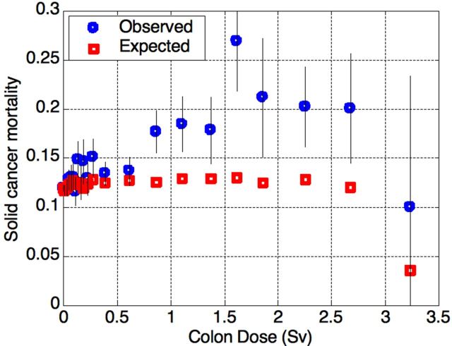
as a function of the exposure D. The results are shown at Fig.3. Because the highest-dose category (above 3 Sv) contains only 20 survivors, the statistical errors were deemed to be excessive. This dose category was excluded from the data fit for its irrelevancy to any model that could be used to describe the data. Finally, the excess mortality ratio (EMR) was calculated according to formula (1a).

Figure 3.

Observed and expected solid cancer mortality (MR) in the LSS cohort, as a function of the exposure 1950-2003. The highest-dose category contains only 20 survivors, and was therefore excluded from the further analysis due to poor statistics.

Ozasa et al. (2012) calculated not EMR but mortality excess relative rate(ERR), taking into account the attained age (age at death) of the survivors. EMR and ERR are somewhat different, though ERR was calculated by the same formula (1a) with mortality ratio substituted by mortality rate.

To illustrate the difference between EMR and ERR, let us consider a demo model. For example, patients at some advanced stage of disease: 2-year study, mortality rate 20% per year, i.e., survival is 80%. In two years the survival is 0.8² = 0.64, which means that 36% of this population is dead. Suppose now that the mortality rate increases by the factor of 2, i.e., by 100%; the corresponding ERR = 1. Now, the survival is 0.6 after one year, then after the second year we have 0.6² survived and 64% dead. So EMR = (0.64 – 0.36)/0.36 yielding EMR= 0.78, while ERR = 1. That is why the data points of Ozasa et al. (2012, Fig. 5) are somewhat higher than at Fig. 3 above.

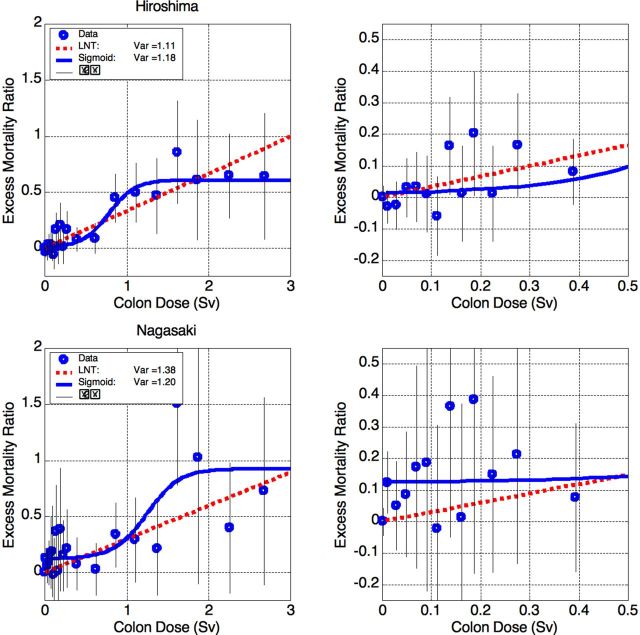
Figure 5.

Excess Mortality Ratio (EMR) for all solid cancers in Hiroshima (top) and Nagasaki (bottom). Left: full data, right: zoomed at low doses. The data are described well by both LNTH and sigmoid. Nagasaki data are somewhat better described by the sigmoidal shape, but the difference is insignificant. The problem of 12% bias is addressed in the text.

We preferred to calculate EMR since (a) it is more straightforward and (b) the statistics are rather poor as will be demonstrated later, so additional division of the data into 21 age categories does not provide new information; on the contrary, it may introduce artifacts due to statistical fluctuations.

The obtained EMR values were fitted by two functions. The first was a one-parametric straight line corresponding to the LNTH:

$$y(X)\hspace{0.17em}=\hspace{0.17em}\alpha \hspace{0.17em}X,\hspace{0.17em}\hspace{0.17em}\hspace{0.17em}\hspace{0.17em}\hspace{0.17em}$$ 2

The second was “sigmoid” s-shaped curve:

$$y(X)\hspace{0.17em}=\hspace{0.17em}a\hspace{0.17em}+\hspace{0.17em}b\hspace{0.17em}/\hspace{0.17em}(1+\exp (-(X-X_0),/\hspace{0.17em}\tau )\hspace{0.17em}\hspace{0.17em}\hspace{0.17em}\hspace{0.17em}\hspace{0.17em}$$ 3

with 4 parameters a (bias), b (saturated value), x₀ (transition center point) and τ (transition width). This shape was chosen to test the hypothesis of a positive threshold for radiation carcinogenesis and provide an alternative to the LNTH. The fits presented at Figs.4 and 5 can be improved further, but we preferred to plot visible-threshold sigmoids, corresponding to local (rather than global) minima of the fit mismatch. The implications are discussed in the next section.

Figure 4.

Excess Mortality Ratio (EMR) for solid cancer mortality in Hiroshima and Nagasaki survivors. Left: full data, right: zoomed at low doses. Both functional descriptions – linear (LNTH) and sigmoidal (s-shaped) – yield nearly equal mismatch Var.

The RERF uses weighted colon dose (measured in units of absorbed dose – Gray) as a reference dose for solid cancer and non-cancer mortality. The weights are ×1 (unity) for gamma-radiation and ×10 for neutrons. Since the above weights are essentially the radiation weighting factors, we use the same variable but prefer to denote it as “equivalent dose” in units of Sievert (Sv). The relevance of the colon dose and possible alternatives, as well as the dose errors, is discussed in the next section.

The errors for EMR stem from statistical uncertainty in the number of solid cancer deaths. The distribution of the number of deaths is not Gaussian but binomial. The statistical problem is: having N experiments with a probability p of a certain outcome – what is the distribution of the number n of certain outcomes? In our case, N is the number of survivors entering the study, and the “certain event” is their death of solid cancer. The number n of solid cancer deaths has therefore binomial (or Bernoulli) distribution with average <n>=N×p (rather intuitive) and standard deviation σ(n)

$$\sigma (n)\hspace{0.17em}=\hspace{0.17em}\surd \hspace{0.17em}[\hspace{0.17em}N\hspace{0.17em}\times \hspace{0.17em}p\times (1-p)].\hspace{0.17em}\hspace{0.17em}\hspace{0.17em}\hspace{0.17em}\hspace{0.17em}$$ 4a

σ(n) is a factor of √(1 – p) less than standard deviation of the Poisson distribution with the same average. For p ~ 0.2 (solid cancer mortality) the difference is not big, but it was taken into account. The standard deviation of the number of deaths for each dose category was calculated according to the formula (4a) with p = MR. Therefore,

σ(MR) = σ(n) / N

and

$$\sigma (EMR)\hspace{0.17em}=\hspace{0.17em}\surd \hspace{0.17em}[MR\hspace{0.17em}\times \hspace{0.17em}(1-MR)/N]\hspace{0.17em}/\hspace{0.17em}M{R}_{\exp ected}\hspace{0.17em}\hspace{0.17em}\hspace{0.17em}\hspace{0.17em}\hspace{0.17em}$$ 4b

The variance of each fit (similar to reduced misfit function χ²) was calculated taking into account the number of degrees of freedom, as

$$Var\hspace{0.17em}=\hspace{0.17em}WRSS\hspace{0.17em}/\hspace{0.17em}(n_{po\mathrm{int}s}\hspace{0.17em}-\hspace{0.17em}{n}_{parameters)},\hspace{0.17em}\hspace{0.17em}\hspace{0.17em}\hspace{0.17em}\hspace{0.17em}$$ 5

where WRSS = Σ[(y_i – y_i(fit)²/σ_i²] is the weighted residual sum of squares, n_points = 20 is the number of fitted data points, and the number of fit parameters is n_parameters = 1 for the LNTH and n_parameters = 4 for the sigmoid. Since our aim was to test the hypothesis of a positive threshold for radiation carcinogenesis and provide an alternative to the LNTH, we did not seek global minima of the mismatch Var for sigmoids but preferred fit parameters corresponding to local minima and apparent thresholds.

RESULTS AND DISCUSSION

Comparing radiation carcinogenesis models

The combined results for excess mortality ratio (EMR) in Hiroshima and Nagasaki are presented in Fig. 4. They are very similar to the results obtained for ERR by Ozasa et al. (2012, Fig. 5). The dose-response relationship for high-dose LSS data (above 1.5 Sv) is more consistent with a plateau shape (flat, dose-independent) rather than a linear increase. This was acknowledged already two decades ago (UNSCEAR 1994, Fig. VI, p. 157). UNSCEAR (1994) provides at least two more cases of radiation carcinogenesis in humans (Figs. IX and XIV on pp. 159 and 162) where the dose-response data reaches saturation at high doses, – or even decreases (Fig. IX). A similar response was also observed in mice for radiation-induced myeloid leukemia (Mole et al. 1983). Cell killing effects can explain the high-dose saturation; there will be fewer “initiating cells” in the high-dose region. This explanation has been qualitatively confirmed by Monte-Carlo simulations (Fornalski et al. 2011); their analysis also shows sigmoidal behavior as the most likely one when a number of linear phenomena are imposed on each other. Moreover, for the A-bomb survivors, the saturation is seen near the threshold of acute effects (~1 Gray) which – together with physical injuries and other factors – could well have led to natural selection of healthier people with stronger immunity that survived until 1950 to enter the LSS cohort. Both Hiroshima and Nagasaki data show EMR maxima at about 1.6 Sv. Although neither of the two maxima is statistically significant, they are conceptually consistent with radiation carcinogenesis for breast cancer (UNSCEAR 1994, p. 159) and the mouse model (Mole et al. 1983).

The results are shown at Fig. 4. Both descriptions, – (a) linear and (b) sigmoid with effective threshold of about 0.3 Sv (as seen at Fig 4, right), – have nearly equal quality with mismatch Var ~1.6 (see the legend box). From the rigorous statistical point of view both fits are rather bad. The deviation of each data point from its fitted value is expected to be about ±σ, so the expected value for the variance is Var~1 for any fit (see (4) above). Var >> 1 means “too bad to be true”, while Var << 1 means “too good to be honest.” Var is chi-squared distributed with good accuracy, as will be shown later. For the corresponding number of degrees of freedom (DOF=n_points – n_parameters), – 19 for the LNTH and 16 for the sigmoid, – the corresponding p-value is p ~ 0.05 (p-value is the probability of obtaining experimental data at least as far from their expected values, as actually observed, assuming that the statistical hypothesis under test is correct). Such p-value should be considered as marginal statistical significance.

The fit quality improves significantly when we process Hiroshima and Nagasaki data separately. Surprisingly, the data yield very different patterns of excess cancer mortality as a function of the exposure.

The Hiroshima data are presented in Fig. 5, top. The Hiroshima survivors comprise about 2/3 of the LSS cohort; therefore, resemblance between Hiroshima and total-LSS data is not surprising. However, the Hiroshima data are statistically consistent (at any reasonable significance level) both with the LNTH and (with similar plausibility) with the sigmoid shape, having an effective threshold of about 0.3 Sv. It is important to stress that neither data point below 0.5 Sv shows significant excess (Fig. 5, top right). The same observation applies regarding the Nagasaki data.

The Nagasaki data are presented in Fig. 5, bottom. The Nagasaki survivors comprise about 1/3 of the LSS cohort, and also the ratio of unexposed survivors is higher than in Hiroshima. As a result, the statistical errors are roughly twice larger. As in Hiroshima, both the LNTH and sigmoidal shapes fit the data well, though the sigmoidal is somewhat better. It should be mentioned here that the parameters of the sigmoid can be varied in rather wide intervals while keeping the fit quality good. This shows that the model parameters are too correlated to attach simple physical meaning to the values obtained.

Although the statistical significance is good, the Nagasaki sigmoidal fit shows apparent rather high dose-independent bias ERR~12%. When this bias is taken into account, the excess below 0.5 Sv for combined Hiroshima + Nagasaki data also becomes statistically insignificant. This dose-independent bias can be attributed to socio-demographic (lifestyle) factors, and also ecological factors. The Nagasaki cohort was formed from essentially two types of population: (1) of the city and (2) of the suburbs and nearby villages. All survivors exposed to more than 5 mSv were within 3 km from the ground zero, while most of those exposed to less than 5 mSv were located at 3 to 10 km distance. Therefore, the exposed population was mostly urban while the unexposed mostly rural. At the time of the bombing, the city of Nagasaki was an important center of heavy industry, with associated air pollution. This can explain higher urban cancer mortality than in the suburbs. As for absence of the urban-rural difference in Hiroshima, there are at least two factors. First, Hiroshima was much less industrialized than Nagasaki. Second, the Hiroshima’s terrain is more even, making the air pollution difference less pronounced. Although this hypothesis cannot be tested using the LSS data, it seems plausible.

Another explanation that should be considered is hormesis, the possible beneficial health effects of low-dose radiation, as discussed in the Introduction. Taking the lowest-dose survivors as a reference leads to “false-positive” excess mortality if the lowest-dose radiation is hormetic. A posteriori, in Hiroshima and Nagasaki, the patterns of EMR as a function of the dose are very different. While the data on Nagasaki survivors may be explained by the lowest-dose hormesis, this is not true for Hiroshima. So we find the socio-demographic explanation of the dose-independent bias more appropriate.

We should reiterate that it is impossible to discard the LNTH, based on the LSS data, which are consistent with both the sigmoidal and the LNTH radiation carcinogenesis models. Moreover, it appears that, given their low statistical power, the LSS data cannot support or contradict the LNTH.

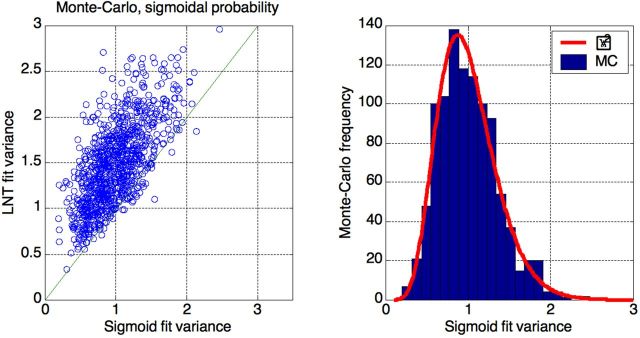
To illustrate the latter statement, we performed Monte-Carlo simulations of the LSS data and their fit. We took raw Hiroshima data, i.e., doses and numbers of survivors (N). Then, assuming sigmoidal EMR values as a function of the dose, as obtained from the fit (Fig. 5, top), we generated 1000 random binomial sequences with given Ns and mortalities. Finally, performed a posteriori fitting with both curves, sigmoidal and LNTH.

The results (Fig.6) show that LSS data are essentially useless for deciding which model is correct. Data that were generated according to sigmoidal (a priori) distribution are well-described by the LNTH (a posteriori) line (average Var ≈ 1.5). As expected, the sigmoidal curve describes the data better, i.e., with smaller mismatch (average Var ≈ 1), but this mismatch is still prohibitively high. E.g., if we use Var >2.0 as a cut value to exclude LNTH, we have to reject the correct sigmoidal description in about 0.5% of cases (7 out of 1000 in this simulation); still we have to accept LNTH in nearly 90% of cases (877 out of 1000 in this simulation).

Figure 6.

Monte-Carlo simulations of the Hiroshima data fit by two curves (sigmoid and LNT). Left: sigmoidal (a priori) data are well-described a posteriori by LNT (y-axis: average Var ~ 1.5). The sigmoidal description is better (x-axis: average Var ~ 1), but dispersion of the fit quality is prohibitively high to exclude LNTH. Right: sigmoid fit variance distribution is well described by scaled χ² function with 16 degrees of freedom.

It seems that the main result of our analysis can be expressed as follows. Given the low statistical power of the LSS, it could not provide evidence in support of the LNTH. The statement of Ozasa et al. (2012) that the data do not support any non-zero threshold is of little value because it cannot be refuted. The principle of refutability demands that any scientific theory or statement should contain information about how to disprove it. As formulated by Popper (1963), “A theory which is not refutable by any conceivable event is non-scientific. Irrefutability is not a virtue of a theory (as people often think) but a vice.”

Quantitative communication of risk

All the above results were obtained, following Ozasa et al. (2012), using the colon dose according to the RERF dosimetry system DS02 (Young and Kerr, 2005). There are two methodological problems with using the colon dose for reference.

• 1) The use of organ dose implicitly assumes a priori some mechanistic model of radiation carcinogenesis – namely that only local irradiation is important. This assumption is plausible but not beyond doubt. What is even more important, the colon is one of the most shielded organs (by the rest of the body). So the question of its relevance as a reference dose for all solid cancers is very unclear.

• 2) Organ dose (and especially colon dose) cannot be determined with good accuracy. The transmission factors (TF) into the body organs are measured on specially-built “phantoms” of human bodies and calculated using very elaborate computer procedures with many known simplifications. All of these results, while reasonable, cannot be verified against real bodies due to regulatory restrictions that prevent such experiments on humans. Even measurements on cadavers may be not very relevant. To the best of our knowledge such experiments have never been performed.

The uncertainties in using colon dose call for considering the external (free-field) dose as probably a more reliable reference. The RERF did not make public the external dose for the groups of survivors, but the breast dose appears to be a good surrogate. While TFs for adult colon are cited by RERF as 0.81 and 0.18 for gamma and neutrons correspondingly (Young and Kerr, 2005, Table 3 at p. 862), TFs for breast are 0.94 and 0.73 – much closer to unity and to each other.

The results are presented at Fig.7, where there are two rather different curves representing essentially the same data. The use of (a) excess mortality ratio (EMR) instead of excess relative rate (ERR) and (b) breast dose instead of colon dose is purely a matter of data presentation. Nevertheless, this may be rather important for risk communication. The RERF reports solid cancer excess risk (ERR) as 42% per Sv (Ozasa et al. 2012, Table 8). If we remain within the LNTH but take (a) EMR instead of ERR, and (b) breast dose instead of colon dose (see Fig. 7), the risk coefficient will be 24% per Sv, i.e. about half the RERF value.

Figure 7.

Relative cancer risk (ERR or EMR) vs. dose (colon or breast). Ozasa et al. (2012) report excess solid cancer risk as ERR/(colon dose)=0.42 Sv^–1 (42% per Sievert, red squares). For the same data, EMR/(breast dose) =0.24 Sv^–1 (24% per Sievert, blue circles).

It should be mentioned here that the excess cancer risk is usually communicated in the terms of excess absolute risk (EAR). EAR is the rate of disease in an exposed population minus the rate of disease in an unexposed population (NRC 2006). The usually cited sex-averaged and age-averaged excess risk value is 5% per Sv as discussed below.

The BEIR-VII report (NRC 2006) cited a preferred overall excess cancer risk estimate for solid cancers deaths as 4100 per 100,000 persons per Gray (4% excess mortality) for males, and 6100 per 100,000 persons per Gray (6% excess mortality) for females. The sex-averaged value of 5% per Gray is usually cited as excess cancer mortality risk for mixed-aged populations. The numbers of solid cancer deaths in the absence of exposure was estimated as 22,100 per 100,000 (males) and 17,500 per 100,000 (females) – see Table ES-1, p. 15. The corresponding EMRs are 4100/22,100 ≈ 0.19 (Sv^–1) for males and 6100/17,500 ≈ 0.35 (Sv^–1) for females. BEIR-VII estimation was based on the value ERR ≈ 0.5 (Sv^–1) (Preston et al. 2003, Table 4) available at that time (1950–1997 follow-up). According to the same guidelines, if EMR and breast dose are used and recent LSS data (1950–2003) exploited, the baseline risk value should be taken as 0.24 Sv^–1 (as discussed above) instead of 0.5 Sv^–1 (Preston et al. 2003). Therefore, the overall LNTH risk should be communicated as about 2% per Sv for males (on the top of 22% mortality of the unexposed population) and about 3% per Sv for females (on the top of 17.5% for the unexposed). After sex-averaging, the excess risk should be communicated as about 2.5% per Sv on the top of ~20% mortality of the unexposed population.

We should stress that although reporting EMR/(breast dose) = 0.24 Sv^–1 instead of ERR/(colon dose) = 0.42 Sv^–1 is the matter of data presentation only, the former is both more comprehensive and more direct. First, the use of excess mortality (how many are expected to die) is intuitively more plausible and comprehensive for the public than “excess relative rate” which affects excess mortality in combination with additional factors. Second, the exposure data are always obtained (and nearly always reported) in terms of the external dose. So the use of the breast dose, which is much closer to the external dose, is more straightforward and therefore preferable.

Neutron discrepancy problem

Finally, let us discuss implications of the problem of “Hiroshima neutron discrepancy” – the apparent difference between the calculated and measured values of thermal neutron activation of radionuclides from materials present in Hiroshima (but not in Nagasaki) at the time of the bombing (Cullings, 2006). This discrepancy has been subject of discussion since the 1960s and was the main motivation for creating the present DS02 dosimetry system (Young and Kerr, 2005). The discrepancy was observed at distances beyond 1 km and increased with distance. At roughly 1.5 km, the calculated neutron doses were at least an order of magnitude lower than the measured doses. However, DS02 did not resolve the problem (Cullings, 2006), and the RERF came to conclusion that the experimental data were unreliable (Young and Kerr, 2005, p. 8).

We assumed here that the neutron discrepancy is real and studied its influence on the Hiroshima results. Colon dose is nearly irrelevant for neutrons because the colon is rather effectively shielded by the body: transmission factor TF(n, colon) of neutrons to colon is according to DS02 as low as TF(n, colon) = 0.18 (for adults), while for gamma-radiation TF(γ, colon) = 0.81 (Table 3 at p. 862). The neutron-to-gamma ratio of TFs is therefore 1:4. Substituting relevant values yields the result that the neutron contribution to the equivalent dose at distances relevant to the neutron discrepancy (~1500 m), is low in spite of the weighting factor 10 and the enhanced neutron yield. But for the breast, TF(γ, breast) = 0.94 and TF(n, breast) = 0.73, so the ratio of TFs (neutron to gamma) is 3:4. Correspondingly, increasing the neutron yield causes considerable changes.

The procedure for recalculating the breast dose was as follows. Gamma and neutron free-in-air absorbed dose values were taken from DS02 for Hiroshima (Young and Kerr, 2005, Table 1 at p. 851). Average gamma-radiation transmission factor TF^b(γ) due to shielding by buildings was taken as TF^b(γ) = 0.6 (Fig. 1 at p. 791), and correspondingly for neutrons, TF^b(n) = 0.55, since neutrons are less penetrating. For adults (survivors above 15 years at the exposure time), the gamma dose was multiplied by TF^b(γ) × TF(γ, breast) = 0.6 × 0.94. The neutron dose was multiplied by TF^b(n) × TF(n, breast) = 0.55 × 0.73, and further by the weighting factor of 10. The same procedure was performed for children (3–15 years) and infants (0–3 years) with corresponding TFs from DS02. The sum of the two above terms (gamma and neutron) yields the equivalent breast dose. The procedure was verified by reconstructing the breast dose from the colon dose and comparing it with the LSS data. The correspondence was found to be excellent (Fig.8) except for the highest doses.

Figure 8.

Breast vs. colon dose for the Hiroshima survivors. Infants: less than 3 years at exposure; children: 3–15 years.

Then the free-in-air neutron dose was increased by factor of 10 for the distance 1500 m and further. In order to keep the neutron dose not-increasing with the distance, the 1500-m value was assigned at 1200-1400 m also. Finally, the new breast dose values were plotted vs. DS02 values, and interpolation was performed. The results are presented at Fig.9.

Figure 9.

Left: re-calculation of the breast dose with enhanced neutron yield. Right: resulting multiplication factor for the breast dose.

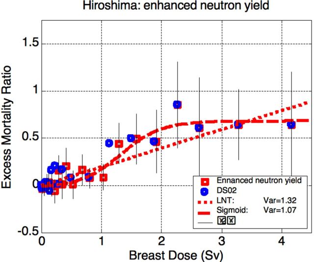
The re-calculated Hiroshima data are shown at Fig.10 (the doses are higher than in Fig. 7 because of the neutron contribution, which is higher in Hiroshima). Somewhat counter-intuitively, ×10 enhancement of the neutron yield leads only to slight shift in the intermediate-dose region with no serious implications. Now the data fit favors somewhat more the sigmoid model (with effective threshold of 0.5 Sv) over the LNTH. However, the difference in the fit qualities is not significant and, as expected from the Monte-Carlo simulations reported above, neither model can be rejected.

Figure 10.

Results for increased neutron yield in Hiroshima. Breast dose is used for reference since colon is heavily shielded from neutrons by the body. The sigmoid yields somewhat better fit than LNTH, but the difference is insignificant. For the sigmoid model of carcinogenesis, effective threshold is at about 0.5 Sv (breast).

CONCLUSIONS

It is often claimed that the data of the atomic bomb survivors life-span study (LSS) support the linear no-threshold hypothesis (LNTH). The analysis reported here shows that this claim should be considered as lacking factual base. The LSS data are equally or better described by the s-shaped dose-response model for radiation carcinogenesis, with threshold dose of about 0.3 Sv and saturation at about 1.5 Sv. Even if the LNTH is used at low dose and dose rates, the estimation of excess cancer mortality should be communicated as 2.5% per Sv (about half of the usually cited value), i.e. cancer mortality increase per Sievert from about 20% (spontaneous cancer mortality) to about 22.5%.

Taking into account (a) the dominant role that the LSS findings played in setting the no-threshold radiation risk assessment paradigm (and consequently – radiation protection standards), (b) the vast scientific evidence supporting effective thresholds (safe dose levels) for radiation carcinogenesis and (c) the high costs, including human costs, of radiation protection in its present form – major revision of the radiation risk assessment paradigm is required.

REFERENCES

- Cullings HM, Levenson ZB, Funamoto S., Teranishi S. 2006. Changes in Atomic Bomb Survivors’ Dosimetry with the New Dosimetry System DS02. Jap. J. Health Phys. 41(4):261–271. [Google Scholar]
- Doss M. 2012. Evidence Supporting Radiation Hormesis in Atomic Bomb Survivor Cancer Mortality Data. Dose Response. 10:584–592 [DOI] [PMC free article] [PubMed] [Google Scholar]
- Feinendegen LE, Pollycove M, Sondhaus CA. 2004. Responses to low doses of ionizing radiation in biological systems. Nonlinearity in Biol. Toxicol. Med. 2: 143–171 [DOI] [PMC free article] [PubMed] [Google Scholar]
- Feinendegen LE, Pollycove M, Neumann RD. 2013. Hormesis by low dose radiation effects: Low-dose cancer risk modeling must recognize up-regulation of protection. In: Baum RP. (Ed.) Therapeutic Nuclear Medicine, Springer 2013, 500 p. ISBN 978-3-540-36718-5 [DOI] [PMC free article] [PubMed] [Google Scholar]
- Fornalski KW, Dobrzyński L., Janiak MK. 2011. A Stochastic Markov Model of Cellular Response to Radiation, Dose-Response 9:477–496 [DOI] [PMC free article] [PubMed] [Google Scholar]
- Jaworowski Z. 1999. Radiation risk and ethics. Physics Today 52(9):24–29 [Google Scholar]
- Jaworowski Z. 2008. The paradigm that failed. Int J Low Radiat 5(2):151–155 [Google Scholar]
- Mole RH, Papworth DG, Corp JM. 1983. The dose-response for X-ray induction of myeloid leukemia in male CBA/H mice, Br. J. Cancer 47:285–291 [DOI] [PMC free article] [PubMed] [Google Scholar]
- National Research Council (NRC). 2006. Health Risks from Exposure to Low Levels of Ionizing Radiation: BEIR VII Phase 2. Washington, DC: The National Academies Press, 424p. [PubMed] [Google Scholar]
- Ozasa K, Shimizu Y, Suyama A, Kasagi F, Soda M, Grant EJ, Sakata R, Sugiyama H, Kodama K. 2012. Studies of the Mortality of Atomic Bomb Survivors, Report 14, 1950–2003: An Overview of Cancer and Noncancer Diseases. Radiation Research 177(3):229–243 [DOI] [PubMed] [Google Scholar]
- Office of Technology Assessment (OTA). 1979. The Effects of Nuclear War. U.S. Government Printing Office, Washington, DC, 20402, p. 111. [Google Scholar]
- Popper K, 1963. Conjectures and Refutations, London: Routledge and Keagan Paul, 1963, pp. 33–39 [Google Scholar]
- Preston DL, Shimizu Y, Pierce DA, Suyamac A, Mabuchid K. 2003. Studies of Mortality of Atomic Bomb Survivors. Report 13: Solid Cancer and Noncancer Disease Mortality: 1950–1997. Radiation Research 160:381–407 [DOI] [PubMed] [Google Scholar]
- Sasaki MS, Tachibana A, Takeda S. 2014. Cancer risk at low doses of ionizing radiation: artificial neural networks inference from atomic bomb survivors. J Radiat Res. 55:391–406 [DOI] [PMC free article] [PubMed] [Google Scholar]
- Socol Y, Dobrzyński L, Doss M, Feinendegen LE, Janiak MK, Miller ML, Sanders CL, Scott BR, Ulsh B, Vaiserman A. 2014. Commentary: ethical issues of current health-protection policies on low-dose ionizing radiation, Dose Response 12:342–348 [DOI] [PMC free article] [PubMed] [Google Scholar]
- Taylor LS. 1980. Some non-scientific influences on radiation protection standards and practice – the 1980 Sievert lecture. Health Phys. 39(6):851–874 [PubMed] [Google Scholar]
- Tubiana MF, Feinendegen LE, Yang C, Kaminski JM. 2009. The linear no-threshold relationship is inconsistent with radiation biologic and experimental data. Radiology 251:13–22 [DOI] [PMC free article] [PubMed] [Google Scholar]
- United Nations Scientific Committee on the Effects of Atomic Radiation (UNSCEAR). 1994. Sources and Efeects of Ionizing Radiation. UNSCEAR 1994 Report to the General Assembly, with Scientific Annexes. NY: United Nations. [Google Scholar]
- United Nations Scientific Committee on the Effects of Atomic Radiation (UNSCEAR). 2000. Sources and effects of ionizing radiation. UNSCEAR 2000 Report to the General Assembly, with Scientific Annexes. NY: United Nations. [Google Scholar]
- United Nations Scientific Committee on the Effects of Atomic Radiation (UNSCEAR). 2013. Sources and effects of ionizing radiation. UNSCEAR 2013 Report to the General Assembly, with Scientific Annexes NY: United Nations. [Google Scholar]
- Young R.W., Kerr R.D. (Eds.) 2005. Reassessment of the Atomic Bomb Radiation Dosimetry for Hiroshima and Nagasaki. Dosimetry System 2002. Hiroshima: The Radiation Effects Research Foundation, 997p. [Google Scholar]