Exploring Valleys without Climbing Every Peak: More Efficient and Forgiving Metabasin Metadynamics via Robust On-the-Fly Bias Domain Restriction

Abstract

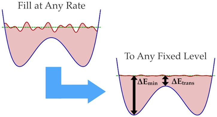
Metadynamics is an enhanced sampling method designed to flatten free energy surfaces uniformly. However, the highest-energy regions are often irrelevant to study and dangerous to explore because systems often change irreversibly in unforeseen ways in response to driving forces in these regions, spoiling the sampling. Introducing an on-the-fly domain restriction allows metadynamics to flatten only up to a specified energy level and no further, improving efficiency and safety while decreasing the pressure on practitioners to design collective variables that are robust to otherwise irrelevant high energy driving. This paper describes a new method that achieves this using sequential on-the-fly estimation of energy wells and redefinition of the metadynamics hill shape, termed metabasin metadynamics. The energy level may be defined a priori or relative to unknown barrier energies estimated on-the-fly. Altering only the hill ensures that the method is compatible with many other advances in metadynamics methodology. The hill shape has a natural interpretation in terms of multiscale dynamics, and the computational overhead in simulation is minimal when studying systems of any reasonable size, for instance proteins or other macromolecules. Three example applications show that the formula is accurate and robust to complex dynamics, making metadynamics significantly more forgiving with respect to CV quality and thus more feasible to apply to the most challenging biomolecular systems.

1. Introduction

Although in principle observing nature carefully over infinite time scales could be sufficient to reveal all physics, it is more practical to design experiments that investigate specific questions by intentionally varying physical parameters in a controlled manner. Similarly in computational modeling, when direct simulation of natural processes by molecular dynamics¹⁻³ is infeasible, specially designed simulations can nonetheless reveal key physics in far less simulation time.⁴⁻⁶ The adaptive enhanced sampling method metadynamics⁷⁻⁹ is one such approach specifically designed for the determination of potentials of mean force (PMFs) by promoting transitions between long-lived metastable states. Metadynamics has been widely applied across chemistry from materials science to biochemistry, but it is still quite young theoretically, with a rigorous proof of convergence appearing only one year ago.¹⁰

Metadynamics works by using a choice of reduced coordinates called collective variables (CVs) to iteratively build a bias that increases the rates of transitions between metastable energy wells; increased transition rates imply decreased sampling autocorrelation and thus improved PMF estimates. Other adaptive methods of the same generation and similar philosophy include the Adaptive Biasing Force^11,12 and Wang–Landau¹³ algorithms, and it is descended from the Local Elevation Method.¹⁴ The degree to which a bias can actually promote those transitions, however, depends on how well the CVs capture the true reaction coordinates. When the CVs are imperfect, the results may not approach the true PMF rapidly, and this is common enough that it is often considered to be the single most relevant limitation preventing application of metadynamics to the study of complex systems.^9,15−18 Furthermore, the cost of building the bias also depends on the complexity of the CVs, scaling with the volume of CV space–i.e., exponentially with CV number. All enhanced sampling methods that rely on CVs share these drawbacks to greater or lesser extents.^6,19,20 This paper describes a new variant of metadynamics, metabasin metadynamics (MBMetaD), that is designed to suffer less from the use of poor quality CVs and to make more practical the use of larger numbers of CVs by judiciously restricting the bias’s domain in CV space. However, in order to discuss the features of metadynamics that we wish to improve with our new method, we must first compare to a more venerable alternative, window-based umbrella sampling.^21,22

Window-based umbrella sampling is stratified sampling applied to simulation.²¹ It is accomplished by running many simulations with different energetic biases that keep each simulation restrained within a different small region, or window, of CV space. These windows are constructed so that the sampled distributions in the windows overlap with one another to cover all of the phase space of interest in a given investigation; this typically involves choosing 1) a scale for each stratified dimension of CV space to set the separation of window centers from one another and 2) a single energy scale to set the strengths of the restraint. Once these are chosen, one then runs simulations in each window, perhaps with some form of replica exchange among the biased walkers.^6,22 After this, the sampling in all of the windows forms a patchwork covering of the CV space that can then be sewn together into a single overall PMF estimate using a method such as Gaussian process regression,²³ the weighted histogram analysis method,²⁴ or the multistate Bennet acceptance ratio.²⁵

Metadynamics, on the other hand, is an auxiliary distribution sampling approach. It functions by iteratively building a bias away from previously visited points to accelerate escape from metastable basins and thereby decrease autocorrelation of sampling on the CV space. In tempered metadynamics,^26,27 the type of metadynamics that converges asymptotically,¹⁰ the bias is constructed by adding Gaussian hills of bias of progressively shrinking height at regular intervals. Overall, a typical case requires choosing 1) the length scale of the hill in each dimension, 2) a single hill energy scale, and 3) a single energy scale for the convergence rate of the bias. After these are chosen, one then runs one or more simulations under an iteratively growing bias, again with the possibility of replica exchange.²⁸⁻³⁰ Once this is done, one can calculate PMFs via their direct connection to the bias in the asymptotic regime or via one of several nonequilibrium reweighting estimators.³¹⁻³³

When stratifying based on a set of CVs is not enough to ensure good sampling over the CV range, one says that there are hidden slow variables (HSVs). When these are present, replica exchange can be inefficient, and sampling in the windows often does not accurately represent true Boltzmann sampling on accessible simulation time scales.^22,34 The free energy differences between windows spaced far apart are pieced together using information from windows between them, making the errors induced by poor sampling in a single window nonlocal. This nonlocality follows the topology of the PMF in a way such that sampling errors in transition regions have large effects on relative free energy estimates between the basins they connect, while errors in basin regions and high energy regions have a more local effect.³⁵ However, unless the HSVs prevent replica exchange or lead to obvious unphysical features in a PMF, the erroneous sampling can easily be mistaken for correct.

The presence of HSVs in metadynamics, on the other hand, typically causes sampling hysteresis that is clearly visible in the bias.^9,17,28 When the CVs are open for modification, this is an advantage because it gives a clear signal that the CVs need improvement. As in window-based umbrella sampling, the effect on PMF estimates is nonlocal, but, unlike in that method, the nonlocal effects from HSV sampling in high-energy regions can affect the estimates of the PMF across all other regions. Specifically, the nonequilibrium bias can drive undesired changes in HSVs that never relax on the time scale of simulation, for instance driving undesired boiling of solvent or an irreversible fluctuation of a protein conformation. That spoils the sampling, making it useless for prediction. Therefore, although hysteresis in the presence of HSVs is a desired behavior in regions of CV space relevant to the process of interest, it is an inconvenience in high-energy regions. It is especially troublesome in complex systems with sensitive dynamical environments and many potential HSVs, e.g., almost all proteins.

Regardless of the presence of HSVs, the simplest form of windowed umbrella sampling scales poorly with the dimensionality of CV space because one typically covers the space with the fixed-volume windows, and the cost of covering space with fixed-volume sets scales exponentially with dimension. This can be ameliorated somewhat by taking a metadynamics-like approach in which one runs simulations only in windows in low-energy regions encompassing the main basins of interest, i.e., a metabasin, gradually learning the shape of the metabasin along the way.³⁶ The metabasin manifold has a lower volume—and often a lower effective dimensionality—than its bounding box, so covering it with windows is less prohibitive than covering the full span of the CV space. No advance knowledge of the metabasin’s shape is required, only an energy scale of interest.

In this paper we propose to emulate this approach for metadynamics. However, our goal and approach differ. Our primary goal with MBMetaD is to prevent driving in high-energy regions to prevent the excitation of HSVs that irreversibly alter sampling. Greater efficiency with many CVs is another benefit and an important one, but it is currently a less pressing issue in the application of metadynamics than the problem of irreversible driving. The strategy differs from adaptive umbrella sampling because metadynamics already acts to fill metabasins from the lowest point out—an initialization logic—and our change is therefore rather to cause metadynamics to drive escape no further and converge once it has filled the metabasin—a termination logic.

The most common approach to this termination in the literature has been to self-limit by slowing down the addition of bias, for instance in self-healing umbrella sampling,³⁷ flat histogram metadynamics,³⁸ and well-tempered metadynamics.²⁶ However, though these can be effective, in such methods the time scales of updating the bias and the energy scale of the self-limiting are tightly coupled, which can make it impossible to simultaneously choose acceptable values for both in complex systems. Most often, one must simply choose to add energy very slowly or, similarly, decrease the rate of energy addition very rapidly to prevent spoiling the dynamics. In either case, this can make the simulations prohibitively expensive. There is therefore a need for a scheme that takes a different approach, sampling a specific energy scale regardless of how quickly bias is added, to empower researchers to make more practically efficient investigations of sensitive systems with metadynamics.

In this paper, we solve the longstanding problem of designing metadynamics to flatten only a region of arbitrary shape, without restricting sampling to that region, in order to design a metadynamics that flattens only up to a chosen energy level and no further regardless of how quickly new bias is added. The approach we take is compatible with all tempering strategies,^10,26,27,39 bias exchange,²⁹ multiple walkers,⁴⁰ and more,^18,30,41,42 functioning as a modular enhancement that can and should be used together with other advances in metadynamics methodology. The task of filling a finite domain has been a pernicious challenge throughout the history of metadynamics.⁴³⁻⁴⁵ When used without proper understanding it can suffer from boundary artifacts. Solutions are available for 1D intervals,^43,44 but the first simple, implemented solutions for rectangular boxes with hard wall boundary conditions in any number of dimensions were first published by McGovern and de Pablo only two years ago.⁴⁵ We independently derived the same corrections in the course of studying the convergence of metadynamics, and here we extend the McGovern–de Pablo approach to time-dependent domains of arbitrary shape with open boundaries. Our method consists of this generalized boundary-corrected metadynamics together with adaptive rules for defining time-dependent domains that represent the metabasins of genuine physical interest in practical metadynamics applications. These rules do not require any a priori estimate of barrier heights in the system. Section 2 details this new method, Section 3 presents results and discussion of three example applications to biomolecular simulation, and Section 4 concludes the paper.

2. Methods

Tempered metadynamics is proven to converge like a specific quasiequilibrium differential equation that depends only on the method and not on underlying system dynamics.¹⁰ Therefore, to describe the design of the new approach that converges on a finite, open-boundary domain, we first define a new shape of hill that gives rise to a differential equation that flattens the energy on any domain. Second, because the domain of interest will only rarely be known ahead of time, we next discuss how to adaptively define these domains over the course of simulation using either a known target basin energy level or an adaptively learned energy level corresponding to the minimal metabasin containing several known points of interest.

In the original metadynamics,⁷ the adaptive bias is constructed as a sum of Gaussian hills centered at previously visited points in CV space, i.e., in 1D

1

where h is an energy-valued hill height, σ is a CV-valued hill width, and the s_ti are the sequence of points in CV space visited at each t_i. To ensure convergence one must sequentially decrease the hill height, for instance using the well-tempered metadynamics (WTMetaD)²⁶ rule

2

where ΔT is a parameter that controls the rate of height decrease. A general theoretical form for metadynamics that can be proven to converge¹⁰ is

3

where G(s, s′) is called the hill kernel and encapsulates the hill shape, and w[V(s, t_n)] is called the global tempering rule and serves as a complement or substitute to the WTMetaD rule for decreasing the hill sizes as time goes on; see for example transition-tempered metadynamics (TTMetaD)²⁷ or the global tempering used in experiment directed metadynamics.³⁹ The new method of this paper is modular with respect to the various tempering rules and only involves redefinition of G(s, s′).

Specifically, consider the case that one knows of some hill kernel G₀(s, s′) that could flatten an entire CV space but would like to flatten a domain D of that CV space instead. Then the MBMetaD rule is to use a hill with two parts

4

where G_Int(s, s′) are hills that would flatten the interior of the domain if it had hard walls, and G_Ext(s, s′) raises the bias level of the exterior in such a way to exactly match the exterior bias level to the bias level of the domain boundary while also exactly counteracting the parts of G_Int(s, s′) that slope into the exterior of the domain. Both are based only on G₀(s, s′) and the domain D. These hills are illustrated in Figure 1.

Figure 1.

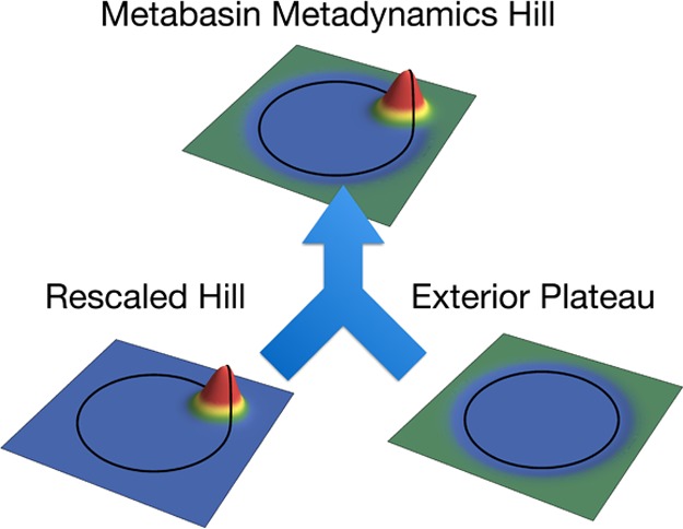
An illustration of a metabasin metadynamics hill function (top, eq 4) on the unit circle near the domain boundary (black lines denote r = 1) and its decomposition into a rescaled hill (left, eq 7) and a low plateau outside of the domain (right, eq 9). The hill is based on a Gaussian of width 1/√10 placed at r = 0.9. The effects of adding rescaled hill and exterior plateau contributions evenly over all points on the unit circle are exact complements, leading to bias updates that are flat everywhere when sampling is flat on the unit circle.

For the first part, we use a close relative to the multiplicative McGovern–de Pablo⁴⁵ rule

5

where I(s; D, G₀) is a boundary-normalized integral of G₀(s, s′) over D for its s′ argument, i.e.

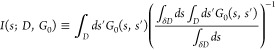6

with δD the boundary of domain D. This integral does not have a closed form solution for domains of general shape, but for Gaussian hills on a rectangular domain it is given by the sum of error functions provided in the paper of McGovern and de Pablo.⁴⁵ The rule eq 5 has the undesirable property that as s′ approaches the boundary of D from the interior, the values of G(s, s′) in the exterior diverge to infinity, making it unsuitable for metadynamics on an open boundary domain. This occurs because I(s; D, G₀) goes to zero quickly as s goes beyond the boundary, so an expedient solution is to modify I(s; D, G₀) such that it falls to a fixed value greater than zero. In MBMetaD, therefore, our form for the first term in eq 4 is

7

with I(s; D, G₀) as above and in the implementation described in this paper f(x) is the simple piecewise polynomial f(x) = x for x ≥ 1 and f(x) = x + 0.5(1–x) ² for x < 1. This choice of f is continuous and differentiable even at x = 1, ensuring that all bias forces will be continuous. I(s; D, G₀) is constant in the interior of the domain and decays to zero outside of the domain, so dividing by f(I(s; D, G₀)) has the effect of leaving hills in the interior unchanged and causing them to bulge out of the domain subtly more than they otherwise would when close to its boundary.

Using only that first part of the hill, the differential equation from the convergence paper¹⁰

8

would predict that the interior of the region would be flattened, but the bias inside would grow indefinitely, forming a steep-walled, flat-topped mesa in the PMF. This would drive all sampling out of the metabasin of interest and is clearly undesirable. The second term in eq 4 ensures that this does not occur. Specifically, we use

9

which plateaus in the exterior of the region with a plateau height equal to the boundary average value of the first part of the new bias. An example is illustrated in the bottom right of Figure 1. Because its height is set to match the bias added to the boundary, it ensures that the exterior bias level always matches the average bias level of the domain boundary. In other words, this part of the bias update pulls sampling into the domain everywhere along the boundary exactly enough to cancel out how the first part of the hill would push sampling out of the domain close to the new hill. Moreover, the plateau is perfectly shaped so that flat quasiequilibrium sampling on the interior of the domain leads to an exactly flat increase of the bias everywhere in CV space. Finally, this term, eq 9, is only nonzero when a hill is added close to the boundary (s′ is close to the boundary), so MBMetaD functions just like normal metadynamics away from those boundaries.

While this scheme might appear technical at first glance, it has a simple multiscale physical interpretation. On a coarse scale, we look at the system through a two-state lens: either the sample is inside or outside the domain. On a fine-grained scale, we look at the points in CV space to a resolution comparable to the length scale σ of the original hill. The metabasin rule, then, corresponds to looking at the CV space using a topology in which all the points inside the domain are resolved to a fine-grained level, while all of the points outside are collapsed into one generic state. The first part of the hill is added to a fine-grained neighborhood of the interior, while the second is added to the entire coarse-grained exterior state—also a single neighborhood, but using the multiscale topology described above instead of the usual metric topology of the CV space.

It is often argued that bias hills should match the Green’s functions for the dynamics, in at least a loose sense,^14,32,46,47 and this is no exception. The simplest way to understand this new hill shape in those terms is to recognize that these hills are also like Green’s functions, but where boundary conditions have been adjusted so that the walls are only partially reflective and any particles that exit the boundary from the interior must be balanced by particles crossing the boundary from the exterior. In the exterior, the constant profile in the far field corresponds to a well-mixed, fixed concentration boundary condition at infinity. The second part is thus related to the quasistationary distribution of a well-mixed domain exterior and therefore retains a natural connection to dynamics.

Up to now we have spoken in terms of a single connected domain, but the development above applies to any disconnected domain just as easily. Simply divide the domain D into its n components D_i and whenever a sample would be added inside a domain D_i, use the above definitions with D_i in the place of D. In the discussion of its physical meaning, consider a 2ⁿ-state coarse-graining rather than a two-state coarse-graining; the new set of states is the Cartesian product of all the sets of two states (interior and exterior) per domain.

When one’s goal is to flatten a PMF in a domain without causing discontinuities, the only domains that can be flattened completely are those with an isoenergetic boundary. Therefore, it is natural to define valid domains by defining a boundary free energy and letting the domain be the set of all CV points with a lower free energy than that boundary energy. Since the zero of free energy is arbitrary, these definitions must be made in terms of an energy difference rather than an energy alone. For instance, in this paper, we will show the use of domains like “all points less than 45 kJ above the minimum free energy”, a known basin free energy level, and “all points less than 15 kJ above the transition barrier between points A and B”, an implicitly defined metabasin energy level. Of course, the choice of domains D_i is rarely possible to make before a simulation. It is often one of the things one would like to discover using metadynamics. For that reason, we also add an on-the-fly mechanism to discover D_i defined in terms of simpler criteria like the examples above.

We solve this problem much as in TTMetaD,²⁷ where we used the bias as an on-the-fly free energy estimator. However, in this case we seek metabasins rather than barriers, and now the bias will not properly approximate the free energy anywhere outside of a previously defined domain. Therefore, we use the nonequilibrium umbrella sampling estimator of Branduardi, Bussi, and Parrinello³² to approximate the domain locations on-the-fly rather than the bias alone. This allows for the discovery of extensions of a domain outside a previously chosen domain, possibly including new disconnected components, regardless of initial conditions. The free energy estimates provide minima, transition barriers, and on-the-fly region selections as described in the next paragraph.

The recipes above have straightforward numerical implementations. I(s; D, G₀) can be calculated by numerical integration on any domain D simply by summing many hills G₀(s, s′) evenly over D, and once it is available f(I(s; D, G₀)) and I(s; D, G₀)/f(I(s; D, G₀)) are simple to calculate. The nonequilibrium umbrella sampling estimator is evaluated using a running histogram accumulated during simulation alongside the bias, free energy minima are trivial to calculate, and the transition barriers are found via breadth-first path search as in TTMetaD.²⁷ These minima and barriers, plus an offset, define the target region energy. The region of interest is then the total set of grid points under that free energy in the current on-the-fly estimate. That set of grid points is then split into connected domains with a standard flood-fill connected components labeling algorithm.⁴⁸ Once these domains are defined, we compute I(s; D, G₀) for each domain and then continue the simulation. Our implementation updates the domain at fixed time intervals with an option not to update the domain each time but to instead also wait until the free energy estimate in the exterior of the region has changed by some set amount. With tempering, the latter corresponds to a logarithmic update schedule that cuts down on unnecessary computational overhead at late times when the domain definition is stable. Each change in domain definition only affects future hill addition, so the previously deposited bias continues to be used unchanged.

Our implementation is a public fork of the PLUMED2 package.⁴⁹ It provides MBMetaD with a minimum based domain or a transition barrier based domain (with transition barriers defined as described in the paper introducing TTMetaD²⁷), using only one additional required input number, the energy offset from the transition or minimum. Two further parameters to control the update schedule and one controlling accuracy of the numerical integration are also available for fine-tuning, but these have general defaults and can be considered optional.

3. Results and Discussion

Our purpose with MBMetaD is to fundamentally change the trade-offs of metadynamics with respect to other methods by giving it a self-limiting mechanism, and thus the remainder of this paper focuses on investigating the self-limiting behavior in three examples. First, we show that it functions as intended all the way through PMF convergence for a simple model biomolecule with imperfect CVs, alanine dipeptide, without negatively affecting convergence efficiency or accuracy. Second, we show that it correctly self-limits in a more complex example, monomeric actin, where the self-limiting is used to achieve more stable and reproducible exploration of conformational space. Finally, we apply it to a membrane transport protein, ClC-ec1, using mediocre CVs to examine its failure modes and in particular show that it retains metadynamics’ attractive property of displaying hysteresis in the domain of interest (rather than harder to recognize errors) even as it prevents the nonequilibrium driving from spoiling the dynamics in other domains.

Our focus in these examples is the self-limiting behavior and reproducibility rather than convergence efficiency or accuracy; self-limiting behavior aimed at improving reproducibility is the sole novel feature introduced in MBMetaD, and the method otherwise behaves much like whatever other metadynamics method it augments. Though the accuracy of metadynamics in practice does deserve further study, it is not a focus of this particular paper.

3.1. Alanine Dipeptide

A standard first test case for new metadynamics methods is blocked alanine dipeptide in vacuo with ϕ and ψ dihedral CVs because the long literature on metadynamics provides excellent guidance on transferring knowledge gained with this model to understanding of the method in more complex systems.^7,26,32 Alanine dipeptide provides a simple case of a system with imperfect separation of time scales between CV dynamics and other relaxations and is thus a minimal test for any adaptive enhanced sampling method that is meant to be robust to memory in the CV dynamics.

These tests modeled alanine dipeptide using the Amber03 force field⁵⁰ and at a constant temperature of 300 K using a Langevin thermostat with a drag of 5 amu/ps. The dynamics were integrated in Gromacs 4.6.1⁵¹⁻⁵⁴ patched with a customized version of PLUMED2⁴⁹ and using a stochastic dynamics leapfrog algorithm with a time step of 2 fs, particle-mesh Ewald summation,⁵⁵ and SHAKE constraints on all bonds.⁵⁶ We performed 32 simulations for each method and parameter set presented. Each simulation began from the same C_7eq conformation, but each set of 32 runs began from 32 distinct initial velocities pseudorandomly generated from distinct random seeds and used 32 distinct Langevin thermostat seeds.

We compared WTMetaD, TTMetaD, and transition-tempered MBMetaD using hill height, width, and rate parameters and tempering parameters as in our previous work introducing TTMetaD.²⁷ The height was 1.2 kJ/mol, the width 0.35 radians, hills were deposited every 120 fs, the TTMetaD parameter ΔT was 2k_BT, and the transition wells for TTMetaD were (−1.25, 1.25) and (1.0, −1.25) in (ϕ, ψ) CV space; for WTMetaD ΔT was 4 k_BT. When using metabasin metadynamics we compared the minimum-based domain definition with relative energy levels of 35.0 and 42.5 kJ/mol and transition-based domain definition with relative energy levels of 7.5 and 15.0 kJ/mol. We chose these values in order to roughly match the two methods based on the approximation that the apparent transition barrier relative to the minimum in these CVs is 27.5 kJ/mol; this makes for clear and direct comparison between the two different styles of domain specification. The higher energy values were chosen as a representative test of the method. The lower energy values were chosen to illustrate how the two domain definitions differ in behavior as the energy excess above the transition barrier becomes low and the PMF is barely flattened over the barrier between the transition wells.

The results for higher energy limits confirm that MBMetaD with either domain definition retains the accuracy and efficiency of TTMetaD in the low-energy regions it is designed to study while giving up all resolution of the high-energy regions it is designed not to explore. Figure 2 shows the replicate-averaged estimated PMFs of regular TTMetaD and the two MBMetaD variants after 8 ns of simulation for comparison; it is evident that the low-lying contours are essentially indistinguishable among the three methods, while the high-energy contours present in the first are simply missing in the latter two. Also as expected, the contours outside of the domain but close enough to be biased are somewhat random and are not optimized over the course of convergence. Figure 3 compares the convergence rates for these methods on the domain of interest in terms of trueness and precision.

Figure 2.

Bias-based free energy estimates averaged over 32 runs of 8 ns for four different metadynamics choices designed to give different levels of resolution of the high-energy regions. Clockwise from top left: WTMetaD, TTMetaD, 15 kJ/mol transition-referenced MBMetaD, 42.5 kJ/mol minimum-referenced MBMetaD. All methods use parameters as defined in the text. Contours are placed every 5 kJ/mol. The estimates are all but identical in low-energy regions despite stark differences in the high-energy regions. WTMetaD is least controllable and gives the most resolution of high energy regions, TTMetaD is more controllable but would give more and more resolution of high energy regions given additional convergence time, and both forms of MBMetaD are fully controllable, converging without resolving the high energy regions.

Figure 3.

Convergence of MBMetaD bias compared to TTMetaD and WTMetaD. Figures on the left show convergence results for the estimated free energy difference between points (−1.25, 1.0) and (1.25, −1.0), the two primary basins, while figures on the right show convergence results for the estimated free energy difference between points (−1.25, 1.0) and (2.1, −1.5), the deeper basin and the lowest free energy barrier point between the two basins. Figures on top show the averaged free energy difference estimates as a function of time, while the lower figures show the standard deviation of the estimates as a function of time. All methods are as described in the text, with the statistics calculated over 32 runs per method. The MBMetaD methods in these figures used energy offsets of 42.5 kJ/mol (minimum referenced) and 15 kJ/mol (transition referenced). For these free energy difference estimates inside the metabasin domain, MBMetaD incurs no convergence accuracy penalty.

However, with lower energy limits, the transition-referenced domain definitions become clearly superior to minimum-referenced domains. This is shown in Figure 4. This is because in the normal case that CVs are imperfect, hidden barriers in HSVs can cause the bias to grow too high in one basin before exploring the next basin.⁹ When this occurs in minimum-referenced MBMetaD, the energy differences from the minimum can therefore appear higher than they should and the estimated domains then become too small. If the intended domain was not much larger than the true metabasin of interest, the bias may not fully flatten all the way between the states of interest until the overestimation corrects itself. On the other hand, when similar overestimation occurs in transition-referenced MBMetaD, the transition barrier estimate also overshoots the true value, so that the domain is made larger by the same amount that the previous error would make it smaller. This systematic cancellation of errors ensures greater stability and better flattening before convergence and, thus better, less autocorrelated sampling and faster convergence. We always recommend using the transition-based rule for adaptive domain restriction when seeking to connect basins.

Figure 4.

Comparison of the convergence of MBMetaD biases using different domain specifications. The MBMetaD methods in these figures used energy offsets of 42.5 kJ/mol (high energy minimum referenced), 35 kJ/mol (low energy minimum referenced), 15 kJ/mol (high energy transition referenced), and 7.5 kJ/mol (low energy transition referenced). The trueness of the MBMetaD methods are all fairly consistent, but the precision of transition-referenced MBMetaD is more robust with respect to choice of domain specification due to the early time cancellation of errors discussed in the text.

In these tests, the desired regions of interest are single large connected domains including both wells. In the high energy tests, the on-the-fly regions begin with large connected domains including both wells and small disconnected satellite domains due to sampling noise in the free energy estimate. As the simulation proceeds and the free energy estimate is refined, new satellites spring up, some disappear, and some connect with and absorb into the main domain. The behavior is the same in the low energy transition-referenced simulation as well. However, in the low energy minimum-referenced simulations, the regions often begin with one primary domain around the basin the simulation is initialized in. In these runs, when a transition to a new well occurs there is a delay before the umbrella sampling estimator registers the discovery of a new low-energy region, but then a domain begins to grow around the new basin. Depending on vagaries of sampling, these domains can either remain separate or join together before the simulation terminates. This reconnection is not efficient, so once again, we always recommend using the transition-based rule for adaptive domain restriction when seeking to connect basins.

3.2. Actin Flattening

Actin is a key component of the cytoskeleton,⁵⁷ but the structural bases and mechanisms of its regulation are only partially understood, even at the monomer level. The monomer is also called globular actin or G-actin, and aspects of it have been studied using metadynamics^58,59 and umbrella sampling.⁶⁰ However, G-actin is a dynamically sensitive protein with a high degree of allostery that can be difficult to design good CVs to investigate and can resist enhanced sampling analysis.⁶¹

A previous paper⁶⁰ used umbrella sampling to investigate nucleotide-dependent G-actin conformational distributions measured in terms of an interdomain distance and torsion (Figure 5) but was unable to reach convergence, presumably due to the presence of HSVs. Attempting to use metadynamics with the same torsion and distance CVs showed hysteresis, confirming the presence of HSVs, but this hysteresis typically involved unexpected and apparently irreversible behavior. Hypothesizing that the CVs were adequate in low-energy regions but inadequate in higher energy configurations, we applied MBMetaD to the problem in order to sample the lowest-lying metastable basins well and learn enough to refine the CVs before investigating further.

Figure 5.

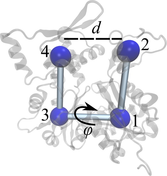
Schematic illustration of the CVs used to investigate nucleotide-dependent actin dynamics, consisting of the distance between subdomains 2 and 4 and the torsion angle between subdomains 2, 1, 3, and 4.

To do this, we performed 8 simulations of WTMetaD with and without adaptive domain restriction for 50 ns each. The simulations were set up as in previous work,⁶⁰ with proteins simulated in NAMD⁶² patched with a customized version of PLUMED2⁴⁹ using the CHARMM22/27 force field with CMAP.⁶³ Our CVs were similar to those in the previous work, consisting of the 2-1-3-4 torsion between the cores of the four actin subdomains—the flatness of the monomer—and the distance between subdomains 2 and 4—the width of the nucleotide binding cleft. However, for the sake of computational efficiency the positions of these subdomains were calculated as the centers of mass of only the backbone and C_β carbons in the subdomain cores rather than the centers of mass of all of the subdomain core atoms. All simulations were initialized from a flattened conformation like that of filamentous actin (PDB ID 2ZWH).⁶⁴ Metadynamics added hills of initial height 0.004184 kJ/mol and widths 0.3 radians and 0.02 nm every 200 fs, with heights sequentially adjusted according to the WTMetaD rule with a bias factor of 10; the MBMetaD domain was defined as every point less than 25.104 kJ/mol above the current estimate of the free energy minimum and was updated every 200 ps if the exterior bias had increased by 2.092 kJ/mol since the last update. A minimum reference is appropriate because the simulations do not study a particular transition but rather the fluctuations about a single basin.

Representative biases and sampling histograms at the end of 50 ns are shown in Figure 6. It is evident that the MBMetaD rule successfully limits the bias to a smaller metastable basin of CV space than the unrestricted WTMetaD does without artificially restricting the sampling to the same basin. The regions selected by MBMetaD correspond to the biased regions. They consist of single primary domains around the starting states together with smaller disconnected domains that spring up wherever the simulation occupies another state long enough. However, the primary purpose of this test is to demonstrate greater simulation repeatability for MBMetaD compared to the WTMetaD reference, investigated in Figure 7.

Figure 6.

Representative sampling from unrestricted WTMetaD (top row) and well tempered MBMetaD (lower two rows) with the same initial conditions (columns) as a function of cleft width (w) and twist angle (θ). In the unrestricted case only bias PMF estimates are shown because sampling and bias are directly related; for MBMetaD both bias PMF estimates (middle row) and sampling histograms (bottom row) are shown.

Figure 7.

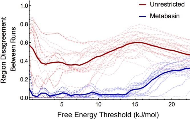
Figure showing the disagreement between the free energy estimates of different runs of like type. Disagreement (y axis) is measured as one minus the ratio of the area of the intersection of the two regions predicted by two different runs to be below a given free energy threshold (x axis) to the area of their union. All PMF estimates are standardized so that their minima are zero. Dashed lines represent the disagreement as a function of free energy threshold for individual pairs, while solid lines indicate their averages. The unrestricted WTMetaD estimates disagree with one another more than the MBMetaD estimates at all free energy levels, showing much improved repeatability for the latter.

This figure demonstrates that overlaps of the biases of different randomly initialized runs are greater in MBMetaD than WTMetaD, i.e., that the sampling is more similar across runs of MBMetaD than WTMetaD, just as desired. The disagreement between predictions of which regions of CV space are below a threshold energy shown in this figure correspond to one minus the ratio of the area of the intersection of the regions to the area of their union; expressed as an integral, this is 1 – ∫ min(I(F_i(s) < F_th), I(F_j(s) < F_th))ds/∫max(I(F_i(s) < F_th), I(F_j(s) < F_th))ds, with F_i and F_j being the PMF estimates from runs i and j, F_th being the threshold energy, and I(f(s) < g) being the indicator of the function f being less than scalar g at point s. This indicates greater stability and more physically meaningful—or at least more easily interpreted—exploration. The nonreapeatable free energy basin predictions seen with unrestricted WTMetaD do not correspond to states that appear biologically relevant or well-populated at equilibrium but rather appear to correspond to metastable traps found only because of overzealous nonequilibrium kicks. The MBMetaD data proved more useful for refining the choice of CVs and designing new simulations, but because refining CVs is a system specific process rather than a matter of MBMetaD methodology, describing that process will be left for future publication focused on the structure of G-actin. For our purposes here, it is sufficient to demonstrate that the method enhances sampling out of well-understood basins repeatably and without applying risky nonequilibrium driving forces in less well understood regions of CV space.

3.3. ClC Antiporter Chloride Transport

Our final example concerns the ClC-ec1 Cl^–/H⁺ exchanger,⁶⁵ a paradigmatic protein of the ubiquitous ClC family.⁶⁶⁻⁶⁹ In this example we will focus on investigating one particular part of the molecular mechanism of chloride transfer: motion of chloride anions in the channel when a key central acidic residue, E148, is protonated. The previous examples showed that MBMetaD is an accurate and effective self-limiting mechanism when the CVs are appropriate in a metastable basin. However, it is often the case that CVs will not be ideal even in the domain of interest, and with this final example we intend to show that MBMetaD continues to have both desirable self-limiting behavior and dynamics with desirable hysteresis in that case. Therefore, in this case our CVs are simply the displacements along the membrane normal direction, z, from each of two chlorides, one closer to the cytosolic side of the membrane, z_cyt, and the other closer to the extracellular side, z_ext, to the center of mass of a central group of protein atoms that is chosen only as a stable reference for the protein frame of reference and has no other intended physical significance. This leaves motion of E148, water fluctuations, helix motion, and other protein environment fluctuations as potential HSVs.

We aim here to compare the function of MBMetaD with unrestricted WTMetaD in estimating PMFs of simultaneous translation of these chlorides throughout the protein, with the mechanism presumed to involve five key chloride states identified in previous structural studies.^67,70,71 First, when z is greater than 1 nm, the chloride is said to be extracellular. Second, when z is near 0.6 nm, the chloride is expected to be in its external binding site. Third, when z is approximately −0.5 nm, it is expected to be in its central binding site. Finally, when z is less than −1, this coordinate does not distinguish well between whether the chloride is in its internal binding site or unbound on the cytosolic side of the membrane.

The ClC model system was set up as a dimer of the wild-type ClC-ec1 structure (PDB: 1OTS) embedded into a lipid bilayer (163 POPE) and solvated with 11,000 TIP3P waters⁷² in a 92 × 92 × 79 ų box under periodic boundary conditions. Protein and lipids were modeled with the CHARMM27 force field;^73,74 long-ranged electrostatic interactions were treated with the Particle Mesh Ewald (PME) method,⁷⁵ and the cutoff distance for the short-ranged interactions from both the Lennard-Jones and the real-space Coulomb interaction was set to be 12 Å. The classical MD simulation was performed using the Gromacs MD package⁵⁴ patched with a customized version of PLUMED2⁴⁹ and a 2 fs time step. The initial configuration of the system was taken from our previous work,⁷⁶ where the system was first equilibrated for 7 ns in the NPT ensemble with a temperature of 310 K and a pressure of 1 atm and then further equilibrated for 10 ns in the NVT ensemble with a temperature of 300 K. Residues E113 in monomers A and B and D417 in monomer A were protonated as suggested by previous calculations,⁷⁷ and E148 in monomer A was also protonated to allow chloride translations from the external to the central site. All other residues were set to their default protonation states.

Metadynamics was applied using the CVs described above for the chloride ions in monomer A only, as previous experiments⁷⁸ showed that each monomer carries out Cl^–/H⁺ exchange independently. Monomer B was still included in the system and simulated as normal, not subject to any direct bias. Hills of initial height 0.2092 kJ/mol and widths 0.035 nm in both dimensions were added each 1 ps. For WTMetaD runs, the well-tempered bias factor was 13, whereas for transition-tempered MBMetaD runs the transition-tempered bias factor was 5 using transition wells (0.45, 1.17) and (1.75, 0.12). MBMetaD domains were targeted to the transition barrier energy between those points plus 12 kJ/mol and were updated every 100 ps if the exterior bias level had changed by 1 kJ/mol. To restrict sampling to cases where the chlorides were in the protein in the appropriate locations in the protein interior, the coordinates of the extracellular and cytosolic-side chlorides were both restrained. The cytosolic-side chloride was restrained to the region −3.24 < x < – 0.93; −2.58 < y < −0.38; 0.09 < z < 2.00, while the extracellular-side chloride was restrained to the region −2.90 < x < 0.70; −2.94 < y < 0.21; −1.49 < z < 0.0. The restraints were implemented as half-harmonic walls with force constants of 200 kJ/(mol Ų).

The free energy estimates given by three simulations using each method after various times, shown in Figure 8, do not correspond to converged potentials of mean force. They reflect the essential randomness of attempting enhanced sampling while neglecting key HSVs and show that MBMetaD prevents the nonequilibrium driving from spoiling the dynamics as it does so frequently in the unrestricted simulations. In the unrestricted case, the metastable band structure seen in the MBMetaD outside of the starting basin is overshadowed by other features in two of the three WTMetaD replicates.

Figure 8.

Bias-based free energy estimates from unrestricted WTMetaD (left column) and transition-tempered MBMetaD (right column) over three runs (rows), each run until features stabilized qualitatively or appeared to be irreparably incorrect. Clockwise from top left, these PMF estimates correspond to 250, 300, 300, 300, 350, and 400 ns of simulation. None appear fully converged, yet the latter are more physically plausible and the former show distinct signs of dynamics gone irrevocably astray in the top and bottom runs (see text for descriptions of the atomistic details behind these unphysical features).

The top left energy profile shows an unexpected and implausible prediction of a sharp well where both chlorides are outside of the protein that is much deeper than any of the expected binding sites, while the bottom left shows a sharp line near z_cyt = 1 that is not seen in any other simulations and also does not correspond to any plausible physics: furthermore, the estimate beyond this line appears to simply be a blob without the expected basin structure for z_ext. In the simulation corresponding to the top unrestricted WTMetaD figure, the trajectory shows that the cystosolic chloride becomes stuck inside the protein between helices that are normally firmly bound together. In the simulation corresponding to the bottom unrestricted WTMetaD figure, one of the main helices unfolds and extends into the solvent: the chloride associates with the helix, and then the nonequilibrium bias ratchets the helix apart by pushing on the chloride, unfolding it turn by turn, before the chloride dissociates and goes into the solvent, with effectively permanent damage done.

Judging by the noticeably different energy scale, it is evident that MBMetaD has expected self-limiting behavior even in this highly challenging and poorly tuned test case, and judging by the fact that the MBMetaD runs do not exhibit the odd behavior seen in the others, it also appears that self-limiting behavior improves robustness to CV quality as predicted. However, it is also clear that the MBMetaD runs in the right column of Figure 8 do not fully agree among one another, showing that it does not cover up core deficiencies in the CVs that can be seen by comparing multiple independent replicates.

The disagreement occurs at the level of which regions of interest are selected on-the-fly, as well. The two topmost right panels substantially agree. However, in the bottom right panel, the final region of interest does not include the upper right quadrant of the allowed CV space. At the time of termination, the simulation was sampling the upper right region but not adding bias. Given time, the histogram correction would ensure that this region would properly register as part of the CV space to bias. Still, as seen in the alanine dipeptide example, it is better to use good CVs and a robust region definition than to rely on long-time convergence of the domains. This reflects the inefficiency of any CV-based enhanced sampling in the presence of HSVs.

Next, mimicking the usual process of checking whether one run might have luckily converged to the correct result despite the gauntlet of possible issues that evidently affected the other runs, we initialized another MBMetaD replicate of length 100 ns beginning with the bias and stored histogram of the top run just before 200 ns to check if the PMF estimate of this replicate would agree with the original copy of the top run after 300 ns. As Figure 9 makes evident, that is not the case. The original run and its branched replicate differ; the former samples configurations in which both chlorides are far from the center of the protein, whereas the other samples configurations in which the cytosolic-side chloride resides in the central pocket. The new replicate primarily explores the initial basin, whereas the original primarily explored the other basins. Motion between the basins is not fully facilitated by the bias because key HSVs are involved in the true barriers between them, and the bias reports that faithfully. MBMetaD correctly reports the presence of these HSVs even as it prevents the less physically interesting and implausible dynamics seen in the unrestricted WTMetaD simulations. The domain restriction rule provides increased safety without covering up essential problems.

Figure 9.

Biased-based free energy estimates from a branched MBMetaD trajectory. The bias-based PMF estimate of the primary trajectory at 200 ns (left) is compared with estimates at 300 ns from direct continuation of that trajectory (middle) and continuation from a new random equilibrated initial conformation (right). The prominent differences between the two show that sampling remains highly autocorrelated on a 100 ns time scale even when biased, a hysteresis that properly indicates the presence of hidden barriers.

4. Conclusions

The new method MBMetaD fundamentally eliminates one of the primary limitations of metadynamics, that adding energy indefinitely causes undesired and irreversible change in many sensitive dynamical systems, by providing an effective and convenient self-limiting mechanism that causes it to fill up to a flexibly defined free energy level and no farther—requiring no a priori estimate of barrier heights but rather estimating them on-the-fly as necessary. This allows for more focused study that should be especially practical when using many CVs at once and incidentally demonstrates a solution to the problem of boundary artifacts in metadynamics on domains of any shape in any number of dimensions. Most importantly, it means that using MBMetaD makes designing good CVs for metadynamics simpler. If energy is no longer added in regions of CV space that are irrelevant to transition mechanisms, the CVs no longer must be carefully tuned there.

Furthermore, having a controlled energy level makes setting the hill height and the tempering rates for WTMetaD and TTMetaD simpler. Current practice requires users to choose their desired energy level by balancing the level of tempering with the initial rate of biasing;^9,26 but the tempering must also be matched to only partially known CV hysteresis time scales, and the biasing rate must also be matched to the only partially known rate of dissipation in the system. Thus, the parameters are overdetermined in a manner depending on unknowns with opaque trade-offs; using MBMetaD to disentangle the choice of final energy level from the choice of tempering rate and hill height can make the choices more straightforward. Additional technical complexity of the method for the implementer is therefore counterbalanced by decreased intuitive complexity for actual application.

By restricting our changes to the hill function alone, we ensure compatibility with many other advances in metadynamics methodology that cannot be discussed in depth here. For instance, the new procedure is compatible in principle with untempered,⁷ well-tempered,²⁶ and transition-tempered²⁷ metadynamics, multiple walkers⁴⁰ and bias exchange,²⁹ driven metadynamics,⁴² experimentally directed (ensemble-biased) metadynamics,^39,79 concurrent metadynamics,³⁰ multiple time steps,⁸⁰ and any choice of CV. It is not compatible with adaptive Gaussian hills³² but is compatible with field-coordinate metadynamics.¹⁸ As noted earlier, it is implemented in a public fork of the PLUMED2 package⁴⁹ and is available with a short guide upon request.

Moreover, there is little reason to think that this strategy applies only to metadynamics. All other adaptive enhanced sampling methods such as the adaptive biasing force^11,12 and orthogonal space random walk⁸¹ approaches can similarly suffer hysteresis effects related to adding reckless driving forces when their parameters are set too aggressively. It may be that adding region-limiting mechanisms like the one presented here may allow for more of those aggressive parameter choices to be used safely, with substantial potential efficiency gains. In each case, one could use the bias and an auxiliary histogram together to determine regions of interest on the fly based on the simple definitions we propose here, such as ‘everything less than 2 kT above the barrier between these two states’.

Finally, we find the physical underpinnings of MBMetaD unexpectedly natural, and we hope they will inspire further thought in the field. The new hills can be understood as approximate Green’s functions of diffusion inside the domain of interest plus an approximate quasistationary distribution in the exterior of the domain. Mathematical work on the foundations of accelerated dynamics^82,83 is finding deep theoretical power in using quasistationary distributions in lifting the Green’s function of a coarse-grained Markov process onto a fine-grained configuration space. Therefore, the MBMetaD hills appear to emerge as approximate mixed-resolution Green’s functions, connecting the worlds of Markov state modeling, accelerated dynamics, multiscale modeling, and CV-based adaptive enhanced sampling in a surprising way.

The authors declare no competing financial interest.

References

- Karplus M.; McCammon J. A. Nat. Struct. Biol. 2002, 9, 646–52 10.1038/nsb0902-646. [DOI] [PubMed] [Google Scholar]
- Adcock S. A.; McCammon J. A. Chem. Rev. 2006, 106, 1589–615 10.1021/cr040426m. [DOI] [PMC free article] [PubMed] [Google Scholar]
- Shaw D. E.; Maragakis P.; Lindorff-Larsen K.; Piana S.; Dror R. O.; Eastwood M. P.; Bank J. A.; Jumper J. M.; Salmon J. K.; Shan Y.; Wriggers W. Science 2010, 330, 341–6 10.1126/science.1187409. [DOI] [PubMed] [Google Scholar]
- Kollman P. Chem. Rev. 1993, 93, 2395–2417 10.1021/cr00023a004. [DOI] [Google Scholar]
- Christ C. D.; Mark A. E.; van Gunsteren W. F. J. Comput. Chem. 2009, 31, 1569–1582 10.1002/jcc.21450. [DOI] [PubMed] [Google Scholar]
- Abrams C.; Bussi G. Entropy 2014, 16, 163–199 10.3390/e16010163. [DOI] [Google Scholar]
- Laio A.; Parrinello M. Proc. Natl. Acad. Sci. U. S. A. 2002, 99, 12562–6 10.1073/pnas.202427399. [DOI] [PMC free article] [PubMed] [Google Scholar]
- Laio A.; Gervasio F. L. Rep. Prog. Phys. 2008, 71, 126601. 10.1088/0034-4885/71/12/126601. [DOI] [Google Scholar]
- Barducci A.; Bonomi M.; Parrinello M. WIRES Comput. Mol. Sci. 2011, 1, 826–843 10.1002/wcms.31. [DOI] [Google Scholar]
- Dama J. F.; Parrinello M.; Voth G. A. Phys. Rev. Lett. 2014, 112, 240602. 10.1103/PhysRevLett.112.240602. [DOI] [PubMed] [Google Scholar]
- Darve E.; Pohorille A. J. Chem. Phys. 2001, 115, 9169. 10.1063/1.1410978. [DOI] [Google Scholar]
- Darve E.; Rodríguez-Gómez D.; Pohorille A. J. Chem. Phys. 2008, 128, 144120. 10.1063/1.2829861. [DOI] [PubMed] [Google Scholar]
- Wang F.; Landau D. Phys. Rev. Lett. 2001, 86, 2050–2053 10.1103/PhysRevLett.86.2050. [DOI] [PubMed] [Google Scholar]
- Huber T.; Torda A. E.; van Gunsteren W. F. J. Comput.-Aided Mol. Des. 1994, 8, 695–708 10.1007/BF00124016. [DOI] [PubMed] [Google Scholar]
- Branduardi D.; Gervasio F. L.; Parrinello M. J. Chem. Phys. 2007, 126, 054103. 10.1063/1.2432340. [DOI] [PubMed] [Google Scholar]
- Tribello G. A.; Ceriotti M.; Parrinello M. Proc. Natl. Acad. Sci. U. S. A. 2010, 107, 17509–14 10.1073/pnas.1011511107. [DOI] [PMC free article] [PubMed] [Google Scholar]
- Sutto L.; Marsili S.; Gervasio F. L. WIRES Comput. Mol. Sci. 2012, 2, 771–779 10.1002/wcms.1103. [DOI] [Google Scholar]
- Tribello G. A.; Ceriotti M.; Parrinello M. Proc. Natl. Acad. Sci. U. S. A. 2012, 109, 5196–201 10.1073/pnas.1201152109. [DOI] [PMC free article] [PubMed] [Google Scholar]
- Lu J.; Vanden-Eijnden E. J. Chem. Phys. 2014, 141, 044109. 10.1063/1.4890367. [DOI] [PubMed] [Google Scholar]
- Wales D. J. J. Chem. Phys. 2015, 142, 130901. 10.1063/1.4916307. [DOI] [PubMed] [Google Scholar]
- Torrie G.; Valleau J. J. Comput. Phys. 1977, 23, 187–199 10.1016/0021-9991(77)90121-8. [DOI] [Google Scholar]
- Kästner J. WIRES Comput. Mol. Sci. 2011, 1, 932–942 10.1002/wcms.66. [DOI] [Google Scholar]
- Stecher T.; Bernstein N.; Csányi G. J. Chem. Theory Comput. 2014, 10, 4079–4097 10.1021/ct500438v. [DOI] [PubMed] [Google Scholar]
- Kumar S.; Bouzida D.; Swendsen R. H.; Kollman P. A.; Rosenberg J. M. J. Comput. Chem. 1992, 13, 1011–1021 10.1002/jcc.540130812. [DOI] [Google Scholar]
- Shirts M. R.; Chodera J. D. J. Chem. Phys. 2008, 129, 124105. 10.1063/1.2978177. [DOI] [PMC free article] [PubMed] [Google Scholar]
- Barducci A.; Bussi G.; Parrinello M. Phys. Rev. Lett. 2008, 100, 020603. 10.1103/PhysRevLett.100.020603. [DOI] [PubMed] [Google Scholar]
- Dama J. F.; Rotskoff G.; Parrinello M.; Voth G. A. J. Chem. Theory Comput. 2014, 10, 3626–3633 10.1021/ct500441q. [DOI] [PubMed] [Google Scholar]
- Bussi G.; Gervasio F. L.; Laio A.; Parrinello M. J. Am. Chem. Soc. 2006, 128, 13435–41 10.1021/ja062463w. [DOI] [PubMed] [Google Scholar]
- Piana S.; Laio A. J. Phys. Chem. B 2007, 111, 4553–9 10.1021/jp067873l. [DOI] [PubMed] [Google Scholar]
- Gil-Ley A.; Bussi G. J. Chem. Theory Comput. 2015, 11, 1077–1085 10.1021/ct5009087. [DOI] [PMC free article] [PubMed] [Google Scholar]
- Bonomi M.; Barducci A.; Parrinello M. J. Comput. Chem. 2009, 30, 1615–1621 10.1002/jcc.21305. [DOI] [PubMed] [Google Scholar]
- Branduardi D.; Bussi G.; Parrinello M. J. Chem. Theory Comput. 2012, 8, 2247–2254 10.1021/ct3002464. [DOI] [PubMed] [Google Scholar]
- Tiwary P.; Parrinello M. J. Phys. Chem. B 2015, 119, 736–742 10.1021/jp504920s. [DOI] [PubMed] [Google Scholar]
- Rosta E.; Hummer G. J. Chem. Theory Comput. 2015, 11, 276–285 10.1021/ct500719p. [DOI] [PubMed] [Google Scholar]
- Thiede E.; Van Koten B.; Weare J.. ArXiv.org, ID 1410.1431, 2014; pp 1–24.
- Wojtas-Niziurski W.; Meng Y.; Roux B.; Bernèche S. J. Chem. Theory Comput. 2013, 9, 1885–1895 10.1021/ct300978b. [DOI] [PMC free article] [PubMed] [Google Scholar]
- Marsili S.; Barducci A.; Chelli R.; Procacci P.; Schettino V. J. Phys. Chem. B 2006, 110, 14011–3 10.1021/jp062755j. [DOI] [PubMed] [Google Scholar]
- Min D.; Liu Y.; Carbone I.; Yang W. J. Chem. Phys. 2007, 126, 194104. 10.1063/1.2731769. [DOI] [PubMed] [Google Scholar]
- White A. D.; Dama J. F.; Voth G. A. J. Chem. Theory Comput. 2015, 11, 2451–2460 10.1021/acs.jctc.5b00178. [DOI] [PubMed] [Google Scholar]
- Raiteri P.; Laio A.; Gervasio F. L.; Micheletti C.; Parrinello M. J. Phys. Chem. B 2006, 110, 3533–9 10.1021/jp054359r. [DOI] [PubMed] [Google Scholar]
- Singh S.; Chiu C.-c.; de Pablo J. J. J. Stat. Phys. 2011, 145, 932–945 10.1007/s10955-011-0301-0. [DOI] [Google Scholar]
- Moradi M.; Tajkhorshid E. J. Phys. Chem. Lett. 2013, 4, 1882–1887 10.1021/jz400816x. [DOI] [PMC free article] [PubMed] [Google Scholar]
- Crespo Y.; Marinelli F.; Pietrucci F.; Laio A. Phys. Rev. E 2010, 81, 055701. 10.1103/PhysRevE.81.055701. [DOI] [PubMed] [Google Scholar]
- Baftizadeh F.; Cossio P.; Pietrucci F.; Laio A. Curr. Phys. Chem. 2012, 2, 79–91 10.2174/1877946811202010079. [DOI] [Google Scholar]
- McGovern M.; de Pablo J. J. Chem. Phys. 2013, 139, 084102. 10.1063/1.4818153. [DOI] [PubMed] [Google Scholar]
- Bussi G.; Laio A.; Parrinello M. Phys. Rev. Lett. 2006, 96, 090601. 10.1103/PhysRevLett.96.090601. [DOI] [PubMed] [Google Scholar]
- Whitmer J. K.; Fluitt A. M.; Antony L.; Qin J.; McGovern M.; de Pablo J. J. J. Chem. Phys. 2015, 143, 044101. 10.1063/1.4927147. [DOI] [PubMed] [Google Scholar]
- Cormen T. H.; Leiserson C. E.; Rivest R. L.. Introduction to Algorithms, 1st ed.; The MIT Press: Cambridge, MA, 1990; p 485. [Google Scholar]
- Tribello G. A.; Bonomi M.; Branduardi D.; Camilloni C.; Bussi G. Comput. Phys. Commun. 2014, 185, 604–613 10.1016/j.cpc.2013.09.018. [DOI] [Google Scholar]
- Duan Y.; Wu C.; Chowdhury S.; Lee M. C.; Xiong G.; Zhang W.; Yang R.; Cieplak P.; Luo R.; Lee T.; Caldwell J.; Wang J.; Kollman P. J. Comput. Chem. 2003, 24, 1999–2012 10.1002/jcc.10349. [DOI] [PubMed] [Google Scholar]
- Berendsen H.; van der Spoel D.; van Drunen R. Comput. Phys. Commun. 1995, 91, 43–56 10.1016/0010-4655(95)00042-E. [DOI] [Google Scholar]
- Lindahl E.; Hess B.; van der Spoel D. J. Mol. Model. 2001, 7, 306–317. [Google Scholar]
- Van Der Spoel D.; Lindahl E.; Hess B.; Groenhof G.; Mark A. E.; Berendsen H. J. C. J. Comput. Chem. 2005, 26, 1701–18 10.1002/jcc.20291. [DOI] [PubMed] [Google Scholar]
- Hess B.; Kutzner C.; van der Spoel D.; Lindahl E. J. Chem. Theory Comput. 2008, 4, 435–447 10.1021/ct700301q. [DOI] [PubMed] [Google Scholar]
- Essmann U.; Perera L.; Berkowitz M. L.; Darden T.; Lee H.; Pedersen L. G. J. Chem. Phys. 1995, 103, 8577. 10.1063/1.470117. [DOI] [Google Scholar]
- Ryckaert J.-P.; Ciccotti G.; Berendsen H. J. J. Comput. Phys. 1977, 23, 327–341 10.1016/0021-9991(77)90098-5. [DOI] [Google Scholar]
- Pollard T. D.; Cooper J. A. Science 2009, 326, 1208–12 10.1126/science.1175862. [DOI] [PMC free article] [PubMed] [Google Scholar]
- Pfaendtner J.; Branduardi D.; Parrinello M.; Pollard T. D.; Voth G. A. Proc. Natl. Acad. Sci. U. S. A. 2009, 106, 12723–8 10.1073/pnas.0902092106. [DOI] [PMC free article] [PubMed] [Google Scholar]
- McCullagh M.; Saunders M. G.; Voth G. A. J. Am. Chem. Soc. 2014, 136, 13053–13058 10.1021/ja507169f. [DOI] [PMC free article] [PubMed] [Google Scholar]
- Saunders M. G.; Tempkin J.; Weare J.; Dinner A. R.; Roux B.; Voth G. A. Biophys. J. 2014, 106, 1710–20 10.1016/j.bpj.2014.03.012. [DOI] [PMC free article] [PubMed] [Google Scholar]
- Leone V.; Marinelli F.; Carloni P.; Parrinello M. Curr. Opin. Struct. Biol. 2010, 20, 148–154 10.1016/j.sbi.2010.01.011. [DOI] [PubMed] [Google Scholar]
- Phillips J. C.; Braun R.; Wang W.; Gumbart J.; Tajkhorshid E.; Villa E.; Chipot C.; Skeel R. D.; Kalé L.; Schulten K. J. Comput. Chem. 2005, 26, 1781–802 10.1002/jcc.20289. [DOI] [PMC free article] [PubMed] [Google Scholar]
- MacKerell A. D.; Feig M.; Brooks C. L. J. Comput. Chem. 2004, 25, 1400–15 10.1002/jcc.20065. [DOI] [PubMed] [Google Scholar]
- Oda T.; Iwasa M.; Aihara T.; Maéda Y.; Narita A. Nature 2009, 457, 441–445 10.1038/nature07685. [DOI] [PubMed] [Google Scholar]
- Accardi A.; Miller C. Nature 2004, 427, 803–7 10.1038/nature02314. [DOI] [PubMed] [Google Scholar]
- Maduke M.; Miller C.; Mindell J. A. Annu. Rev. Biophys. Biomol. Struct. 2000, 29, 411–438 10.1146/annurev.biophys.29.1.411. [DOI] [PubMed] [Google Scholar]
- Dutzler R.; Campbell E. B.; Cadene M.; Chait B. T.; MacKinnon R. Nature 2002, 415, 287–294 10.1038/415287a. [DOI] [PubMed] [Google Scholar]
- Jentsch T. J. Crit. Rev. Biochem. Mol. Biol. 2008, 43, 3–36 10.1080/10409230701829110. [DOI] [PubMed] [Google Scholar]
- Stölting G.; Fischer M.; Fahlke C. Front. Physiol. 2014, 5, 378. 10.3389/fphys.2014.00378. [DOI] [PMC free article] [PubMed] [Google Scholar]
- Dutzler R.; Campbell E. B.; MacKinnon R. Science 2003, 300, 108–112 10.1126/science.1082708. [DOI] [PubMed] [Google Scholar]
- Feng L.; Campbell E. B.; Hsiung Y.; MacKinnon R. Science 2010, 330, 635–641 10.1126/science.1195230. [DOI] [PMC free article] [PubMed] [Google Scholar]
- Jorgensen W. L.; Chandrasekhar J.; Madura J. D.; Impey R. W.; Klein M. L. J. Chem. Phys. 1983, 79, 926. 10.1063/1.445869. [DOI] [Google Scholar]
- MacKerell A. D.; Bashford D.; Bellott M.; Dunbrack R. L.; Evanseck J. D.; Field M. J.; Fischer S.; Gao J.; Guo H.; Ha S.; Joseph-McCarthy D.; Kuchnir L.; Kuczera K.; Lau F. T. K.; Mattos C.; Michnick S.; Ngo T.; Nguyen D. T.; Prodhom B.; Reiher W. E.; Roux B.; Schlenkrich M.; Smith J. C.; Stote R.; Straub J.; Watanabe M.; Wiórkiewicz-Kuczera J.; Yin D.; Karplus M. J. Phys. Chem. B 1998, 102, 3586–3616 10.1021/jp973084f. [DOI] [PubMed] [Google Scholar]
- Feller S. E.; MacKerell A. D. Jr. J. Phys. Chem. B 2000, 104, 7510–7515 10.1021/jp0007843. [DOI] [Google Scholar]
- Darden T.; York D.; Pedersen L. J. Chem. Phys. 1993, 98, 10089. 10.1063/1.464397. [DOI] [Google Scholar]
- Wang D.; Voth G. A. Biophys. J. 2009, 97, 121–131 10.1016/j.bpj.2009.04.038. [DOI] [PMC free article] [PubMed] [Google Scholar]
- Faraldo-Gómez J. D.; Roux B. J. Mol. Biol. 2004, 339, 981–1000 10.1016/j.jmb.2004.04.023. [DOI] [PubMed] [Google Scholar]
- Robertson J. L.; Kolmakova-Partensky L.; Miller C. Nature 2010, 468, 844–847 10.1038/nature09556. [DOI] [PMC free article] [PubMed] [Google Scholar]
- Marinelli F.; Faraldo-Gómez J. Biophys. J. 2015, 108, 2779–2782 10.1016/j.bpj.2015.05.024. [DOI] [PMC free article] [PubMed] [Google Scholar]
- Ferrarotti M. J.; Bottaro S.; Pérez-Villa A.; Bussi G. J. Chem. Theory Comput. 2015, 11, 139–146 10.1021/ct5007086. [DOI] [PubMed] [Google Scholar]
- Zheng L.; Chen M.; Yang W. Proc. Natl. Acad. Sci. U. S. A. 2008, 105, 20227–32 10.1073/pnas.0810631106. [DOI] [PMC free article] [PubMed] [Google Scholar]
- Le Bris C.; Lelièvre T.; Luskin M.; Perez D. Monte Carlo Methods Appl. 2012, 18, 119–146 10.1515/mcma-2012-0003. [DOI] [Google Scholar]
- Lelièvre T.; Nier F. Anal. PDE 2015, 8, 561–628 10.2140/apde.2015.8.561. [DOI] [Google Scholar]