Variability and Constancy in Cellular Growth of Arabidopsis Sepals^,

The growth of cells in the developing sepal is highly variable, but all cells exhibit a surprisingly common, asynchronous maximum growth rate relative to their size.

Abstract

Growth of tissues is highly reproducible; yet, growth of individual cells in a tissue is highly variable, and neighboring cells can grow at different rates. We analyzed the growth of epidermal cell lineages in the Arabidopsis (Arabidopsis thaliana) sepal to determine how the growth curves of individual cell lineages relate to one another in a developing tissue. To identify underlying growth trends, we developed a continuous displacement field to predict spatially averaged growth rates. We showed that this displacement field accurately describes the growth of sepal cell lineages and reveals underlying trends within the variability of in vivo cellular growth. We found that the tissue, individual cell lineages, and cell walls all exhibit growth rates that are initially low, accelerate to a maximum, and decrease again. Accordingly, these growth curves can be represented by sigmoid functions. We examined the relationships among the cell lineage growth curves and surprisingly found that all lineages reach the same maximum growth rate relative to their size. However, the cell lineages are not synchronized; each cell lineage reaches this same maximum relative growth rate but at different times. The heterogeneity in observed growth results from shifting the same underlying sigmoid curve in time and scaling by size. Thus, despite the variability in growth observed in our study and others, individual cell lineages in the developing sepal follow similarly shaped growth curves.

Cells undergo multiple rounds of growth and division to create reproducible tissues. In some plant tissues, such as expanding cotyledons, reproducibility can occur on a cellular level during specific intervals of development, where cotyledon cells exhibit uniform cellular growth (Zhang et al., 2011). However, several studies on cell division and growth in other developing plant tissues have demonstrated that plant cells exhibit considerable cell-to-cell variability during development (Meyer and Roeder, 2014). For example, in both the Arabidopsis (Arabidopsis thaliana) meristem and leaf epidermis, cells show spatiotemporal variation in individual cell growth rates (GRs; Asl et al., 2011; Elsner et al., 2012; Kierzkowski et al., 2012; Uyttewaal et al., 2012). Furthermore, cell divisions have been observed with marked randomness in their timing and orientation (Roeder et al., 2010; Besson and Dumais, 2011; Roeder, 2012). In this study, we identify a hidden, underlying pattern in the seemingly random GR (Box 1) of cells during the formation of sepals in Arabidopsis.

Box 1.

Definitions of GR terms. (For details on the calculations, see “Materials and Methods.”)

Plant cell growth is defined as an increase in cell size due to an irreversible expansion of the cell wall. Neighboring cells physically accommodate one another during plant growth because their cell walls are glued together with a pectin-rich middle lamella, which prevents cell mobility. The cell wall is a thin, stiff layer composed of a polymer matrix including cellulose, hemicellulose, and pectin (Somerville et al., 2004; Cosgrove, 2005). Plant cells change their size and shape by modifying their turgor pressure and/or the mechanical properties of their walls, such as elasticity, plasticity, and extensibility. Growing plant cells exert forces on their neighbors through their walls, and cell wall stresses created by these forces feed back to alter the growth anisotropy (Hamant et al., 2008; Sampathkumar et al., 2014). Although these feedbacks can coordinate growth, they may also amplify differences in growth between neighboring cells (Uyttewaal et al., 2012).

Two competing computational models have proposed explanations of the cellular heterogeneity observed in growing tissues by making different assumptions about how cells grow. In the first, it is assumed that relative growth rates (RGRs) of all cells are uniform in space and time, whereas variation in the timing of division causes the heterogeneity of cell sizes (Roeder et al., 2010). This model suggests that cell divisions cut the sepal into semiindependent cells, which grow uniformly within the expanding organ (Kaplan and Hagemann, 1991). The second model postulates the reverse process: timing of cell division is uniform, but cellular growth is variable and depends on the size of the cell (Asl et al., 2011). This model suggests that cells are autonomous. Currently, there is biological evidence for both models. Variability in cell division timing is observed in sepals and meristems, whereas variability in cellular GRs has been observed in leaves and meristem cells (Reddy et al., 2004; Roeder et al., 2010; Asl et al., 2011; Elsner et al., 2012; Kierzkowski et al., 2012; Uyttewaal et al., 2012). Thus, the debate on how the growth of individual cells within an organ relates to one another remains unresolved.

The identification of underlying patterns in noisy cellular growth processes is challenging. Technical difficulties include the capability for cellular-resolution imaging of the tissue at sufficiently small time intervals. Previous studies (Zhang et al., 2011; Elsner et al., 2012; Kierzkowski et al., 2012) did not image and track individual cells, or they had a coarse time resolution, with 11- to 48-h intervals between images, which may have hidden important temporal dynamics. We studied growing cells in the Arabidopsis sepal, which allows for live imaging with cellular resolution at 6-h intervals (Roeder et al., 2010). The sepal is the leaf-like outermost floral organ of Arabidopsis (Fig. 1) with four sepals of stereotypical size produced per flower. Its accessibility for live imaging makes the sepal an excellent system for studying organogenesis (Roeder et al., 2010, 2011, 2012; Qu et al., 2014). Sepals exhibit high cellular variability in the timing of division and endoreduplication, an alternative cell cycle in which a cell replicates its DNA but fails to divide (Roeder et al., 2010). Furthermore, quantifying cell growth in sepals may shed light on growth mechanisms of other plant organs, such as leaves (Poethig and Sussex, 1985; Roeder et al., 2010).

Figure 1.

Diverse sizes of Arabidopsis sepal cells. A, Four sepals (s) are the outermost green leaf-like floral organs in Arabidopsis. B and C, Scanning electron micrographs of a mature Arabidopsis sepal show that the outer epidermal cells have a wide range of sizes. Asterisks mark some of the largest cells (giant cells) that can span 1/4 the length of the sepal. Scale = 100 µm.

Another key challenge in analyzing cellular growth is the identification of trends in noisy data. Inaccuracies in data acquisition, such as segmentation errors, and noisy growth of individual cells can hide meaningful spatiotemporal trends in growth. GRs measured over longer time intervals will have reduced noise, but they may also obscure important temporal dynamics. Alternatively, previous studies have examined growth of the whole organ or its subregions to avoid cellular noise (De Veylder et al., 2001; Mündermann et al., 2005; Rolland-Lagan et al., 2005, 2014; Kuchen et al., 2012; Remmler and Rolland-Lagan, 2012). However, precise cellular patterns are not resolved. In our study, we use cellular resolution data to define spatially averaged kinematics while keeping the full temporal resolution to identify course-grained spatial trends in the dynamics of cellular growth (Box 1).

We analyze the relationships among the growth of individual cell lineages in a developing Arabidopsis sepal by live imaging and computational analyses. We have developed continuous low-order displacement fields to represent the spatially averaged kinematics of the sepal (Box 1). We find that the growth of the tissue surface area, cell lineage area, and wall length follows S curves, suggesting that their GRs vary over time. Additionally, we find that there is a linear correlation between the maximum GR (i.e. size increase per hour) and the size of the cell. We furthermore find that each sepal cell lineage reaches the same maximum RGR (i.e. GR divided by size). However, each cell reaches the maximum RGR at a different time during its development, generating the observed heterogeneity. Thus, we find underlying similarities in the growth curves of sepal cells.

RESULTS

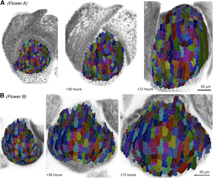
To determine how the growth of plant cells within a tissue relate to one another, we analyzed the growth of sepal epidermal cells by live imaging, developing flowers at 6-h intervals. We tracked the cell lineages using the MorphoGraphX (http://www.mpipz.mpg.de/MorphoGraphX/) image processing and analysis software (Fig. 2; Supplemental Videos S1 and S2; Supplemental Fig. S1; Kierzkowski et al., 2012; Barbier de Reuille et al., 2015). In MorphoGraphX, we extracted a surface mesh from each image and projected the respective fluorescent nuclear and plasma membrane markers (Supplemental Fig. S2; for details, see “Materials and Methods”). The cells were then segmented, their lineages were tracked, and their growth was measured on the surface mesh. Thus, our growth analysis is based on complete information about the size and location of each cell and each of its descendants every 6 h for at least 66 h during the development of the sepal. We analyzed four flowers (arbitrarily named A–D for convenience) including more than 600 cells. Flower A shows a lateral sepal, and flowers B, C, and D show medial sepals. All flowers showed the same overall trends; flowers C and D are presented in the supplement.

Figure 2.

Cell lineage tracking in live images of growing Arabidopsis sepals. Segmented cells and tracked cell lineages at an initial time point, after 36 and 72 h for a lateral sepal in flower A (A) and a medial sepal in flower B (B). Each segmented cell in the figure is colored according to the lineage, which means that cells with the same mother have the same color. More than one lineage can have the same color. The segmented cells (colored) are displayed on top of the original fluorescent plasma membrane and nuclear data (gray). Scale = 50 µm.

Filtering Growth Noise with a Continuous Low-Order Displacement Field

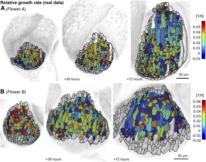
Previous studies have shown that there are striking differences in GRs between neighboring cells in leaves and meristems (Asl et al., 2011; Elsner et al., 2012; Kierzkowski et al., 2012). Likewise, in sepals, we found that the RGRs (i.e. GR divided by cell area) of cell lineages over consecutive 6-h intervals were noisy, and that neighboring cells commonly had different GRs (Fig. 3; Box 1; Supplemental Videos S3 and S4; Supplemental Fig. S3). We considered the growth of cell lineages instead of individual cells so that we could include dividing cells in the analysis. If a cell divided during the time interval, we summed the areas of the daughter cells for the calculations. Similar to leaf cells (Elsner et al., 2012), GRs of sepal cells also changed in time, such that a fast-growing cell in one interval might grow slowly in the next interval, and vice versa. Although much of this variability in GR was attributed to biological processes, we estimated about 20% is due to segmentation errors (see “Materials and Methods”). We therefore spatially averaged the kinematics of cells to identify trends in the growth data. Each trend initially identified in the spatially averaged data was subsequently assessed in the real data.

Figure 3.

The RGR for each cell/lineage computed over a 6-h interval for flowers A (A) and B (B) is noisy, varying greatly from cell to cell. The colormap displays the average RGR_i, which is computed by comparing cell areas A_i and A_i+1 at two subsequent time points t_i and t_i+1 as RGR_i = ln(A_i+1 / A_i) / (t_i+1 − t_i). RGR_i is displayed on the cells of the sepal at time t_i, showing the growth in the following time interval.

To determine spatially averaged kinematics, we used continuous low-order displacement fields u(X, t) (Box 1; for details, see “Materials and Methods”). We were able to apply a continuous displacement field to represent tissue growth because the walls of neighboring plant cells cannot slip relative to one another, and connectivity in the tissue is preserved. For each flower, we defined a reference time point image (i.e. a time point that contains the highest number of shared landmarks among the live-imaging series). For each time point t_j, we used the centers of shared cells and wall segments between that image and the reference image as landmark points to derive the best-fitting low-order function u(X, t_j) among linear, quadratic, and cubic models (for details, see “Materials and Methods”). In all cases, the number of data points was considerably larger than the number of fitting parameters. When choosing the best-fitting model, we avoided overfitting by selecting the model according to the Akaike information criterion (Burnham and Anderson, 2002).

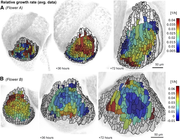
Global low-order displacement fields spatially average growth by smoothing and approximating the change of location of the cell’s landmark points. Using these low-order displacement fields and the cell shapes in the reference time point, we calculated a new set of cell areas and wall lengths for each time point, giving us an averaged data set. This data set was compared with the real data, which are derived directly from the live imaging (Fig. 3). In the averaged data, we were able to observe smooth changes in GRs between contiguous cells (Fig. 4; Supplemental Videos S5 and S6; Supplemental Fig. S4). Due to the spatial averaging, we do not see large variations in the GRs of neighboring cells. However, we often observed that growth varied in time: fast-growing regions could become slow, whereas slow-growing regions could become fast.

Figure 4.

A low-order displacement field smoothens growth. The RGR for each cell lineage using the spatially averaged data for flowers A (A) and B (B) is considerably less noisy than the same quantity extracted from the real data (Fig. 3). The colormap displays the average RGR_i = ln(A_i+1 / A_i) / (t_i+1 − t_i). The cell areas A_i and A_i+1 at two subsequent time points t_i and t_i+1 are computed with the low-order displacement fields u(X, t_i) and u(X, t_i+1), respectively. RGR_i is displayed on the cells of the sepal at time t_i, showing the growth in the following time interval.

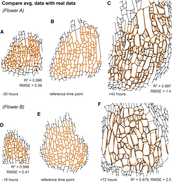
To test whether the displacement field accurately described the growth of the sepal cell lineages, we initialized the cell outlines from the reference time point and grew them in silico according to our calculated deformation gradient. We compared the resulting spatially averaged cell lineages with the real cell lineages that we had measured during live imaging (Fig. 5; Supplemental Fig. S5). The quality of the fit was quantified with the coefficient of determination (R²) and the RMSE. Strikingly, the low-order displacement fields u(X, t_j) fit each flower well (flower A: R² > 0.98 and RMSE < 1.5 μm; flower B: R² > 0.97 and RMSE < 2.6 μm).

Figure 5.

Spatially averaged kinematics fits the real data well. Comparison of the predicted cell lineage growth using the continuous low-order displacement fields u(X, t_j; orange lines) with the real imaging data (black lines) at time points 30 h before (A) or 42 h after (C) the reference time point (B) for flower A and 18 h before (D) or 72 h after (F) the reference time point (E) for flower B. Note that the predicted and real data match remarkably well as the coefficient of determination (R²) is close to 1 and the root mean squared error (RMSE) is low. To simplify the comparison visually in the figure, each wall segment is represented as a straight line. The prediction is for cell lineages and does not take into account cell division. At time points before the reference time, the predicted data contain cells, which have not divided yet in the real data, such that two predicted cells may match one real cell. At time points after, the opposite is the case, such that several real cells may match one predicted cell. For the real imaging data, we show these additional walls as black dashed lines. We do not expect the prediction to match these walls, as they did not exist in the reference time point.

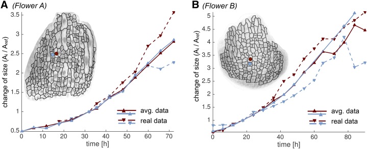
We further compared the data obtained from images and the spatially averaged data computed from the low-order displacement fields for individual cells. Occasionally, we observed neighbors, in which one cell grew faster than the spatially averaged prediction while its neighbor grew slower than the predicted rate (Fig. 6). This substantiates that the displacement field is a good spatial average of the actual data. As expected, we also observed that the real data were considerably noisier than the spatially averaged data in most cases (Fig. 6).

Figure 6.

Spatially averaged kinematics balance out fast and slow growing cells. We show real (dashed) and spatially averaged (solid) growth curves for two neighboring cells (red and blue). The location of the two cells is shown in the inset (red and blue dots). We observe that one cell grows faster than in the spatially averaged growth curve, whereas the other one grows slower. We define the growth curves as cell lineage area (A_i) at time t_i divided by cell area (A_ref) at the reference time point t_ref plotted against time.

Uniform Growth in Space Is a Good Approximation for Sepal Cell Lineage Growth

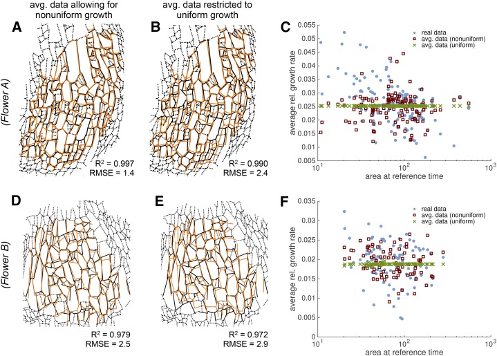
In our previous simple geometric model (Roeder et al., 2010), we approximated sepal growth as uniform in space and time, and suggested that cell size diversity resulted from differences in cell cycle duration. To determine how much sepal cell lineage growth deviates from the uniform growth hypothesis, we defined a cubic displacement function u(X, t_j) with the constraint of having uniform growth in space for the whole sepal, such that the area of each cell lineage increased by the same proportion. We used the same landmark points as for the previous unconstrained displacement field u(X, t_j). To optimize the fit, we minimized the distance from the displaced landmark points to the real landmark points as in the unconstrained fit. To ensure uniform growth, we additionally minimized the sd of the cell area increase. Since we fitted u(X, t_j) independently for each time point t_j, the GR could vary in time. To compare with the real growth of the sepal, we again took the cell outlines from the reference time point and grew them as the tissue would grow according to the uniform growth hypothesis to produce predicted cell lineages and walls. Remarkably, the cell lineages predicted by uniform growth matched considerably well with the real cell lineages that we measured by live imaging (flower A: RMSE = 2.4 μm, R² = 0.990; flower B: RMSE = 2.9 μm, R² = 0.972; Fig. 7, B and E; Supplemental Fig. S6). However, the match was not quite as good as the match with the spatially averaged cells from the previous unconstrained low-order displacement field u (flower A: RMSE = 1.4 μm, R² = 0.997; flower B: RMSE = 2.5 μm, R² = 0.979; Fig. 7, A and D; Supplemental Fig. S6). It is surprising how well the uniform growth displacement field fits despite the fact that the real and spatially averaged RGRs were not uniform (Fig. 7, C and F; Supplemental Fig. S6). This suggests that there might have been compensation or averaging between cell lineages such that the overall growth is approximately uniform.

Figure 7.

Uniform growth in space predicts cellular growth. Comparison of various growth prediction methods (orange lines) with the real imaging data (black lines). A and D, The continuous low-order displacement field prediction (orange lines) for flowers A (A) and B (D) best match the data (black lines). These images replicate Fig. 5, C and F. B and E, Predictions (orange lines) from a displacement field with the additional constraint to have uniform growth in space (but not time), such that the relative increase in cell area is uniform, also matches well with the real data (black lines). It matches almost as well as the unconstrained displacement field (R² and RMSE). For the real imaging data, we show additional walls, which did not exist in the reference time point or were not considered there (black dashed lines). C and F, Graph of the average RGR relative to the cell area at the reference time shows that the real data (blue dots) and the spatially averaged data (red squares) vary greatly around the uniform RGR (green crosses) used in the prediction for flowers A (C) and B (F).

Tissue, Cell Lineage, and Cell Wall Growth Curves Fit S Shapes

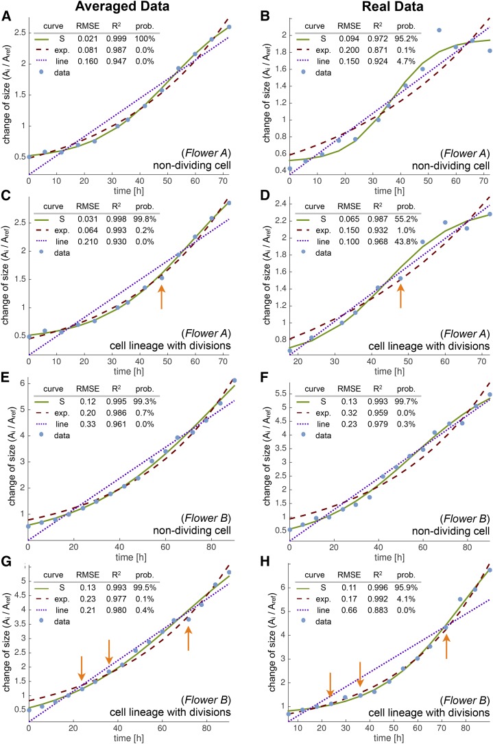
We examined the tissue growth curves as well as those of individual cell lineages and cell walls to determine how the GR changes in time. The tissue growth curves were calculated by taking the sum of the areas of the cell lineages at a given time point and dividing by the sum of the areas of the same cell lineages in the reference time point. To test which function most accurately captures GR changes, we assessed whether a linear, exponential, or sigmoid (S) curve best fit the growth data. In each case, an S curve best fit the tissue growth curves (R² > 0.996 and RMSE < 0.07 in all cases; Fig. 8; Supplemental Fig. S7). Growth data for individual cell lineage areas and individual cell wall segments also best fit S curves (Fig. 9; Supplemental Figs. S8 and S9). We used the Akaike information criterion to calculate the probability that each curve type represented the data (for details, see “Materials and Methods”). In each case, the probability of the S curve was highest, although in some individual cells, the linear fit was a close second (Fig. 9D). The fit of these growth curves to an S shape implies that the GR initially accelerates until it reaches a maximum at time t_m and starts to decelerate (Fig. 8C). Similarly, the RGR (i.e. GR divided by area) increases until it reaches a maximum at time t_x and decreases afterward (Box 1; for details, see “Materials and Methods”).

Figure 8.

Tissue growth curves fit S shapes. We compare the tissue growth (blue dots) with fits to linear (blue dotted line), exponential (red dashed line), and S (green line) curves for flowers A (A) and B (B). In all cases, the S curve fits very well (low RMSE values and R² values close to 1). Probabilities computed with the Akaike information criterion clearly show that the S curve is the most likely fit to the data. C, Sketch of a representative S curve (blue) and its corresponding RGR (yellow). We focus on two relevant time points on the curves: the time where the GR is maximal (t_m), and the time where the RGR is maximal (t_x). We define the growth curves as tissue area (A_i) at time t_i divided by tissue area (A_ref) at the reference time point t_ref plotted against time.

Figure 9.

Individual cell lineage growth curves fit S shapes. We show growth (blue dots) for individual cell lineages of flowers A (A–D) and B (E–H) using the spatially averaged (A, C, E, and G) and real (B, D, F, and H) data. We compare fits to linear (blue dotted line), exponential (red dashed line), and S (green line) curves. We chose growth curves with as many data points as possible to reduce errors from the fit. In all cases, the S curve fits very well (RMSE and R² values). Probabilities computed with the Akaike information criterion show that the S curve is the most likely fit to the data, although a linear function was a close second for some cells (D). We consider nondividing (A and B, E and F) and dividing (C and D, G and H) cells. Cell divisions are marked with orange arrows but did not have a major effect on the lineage growth curves. We define the growth curves as cell lineage area (A_i) at time t_i divided by cell area (A_ref) at the reference time point t_ref plotted against time.

Cell Division Increases Variability in Cell Sizes, But Does Not Have a Major Effect on the Growth Curves

As we have been considering the growth of cell lineages, and not taking into account cell division, we next looked at whether cell division has an effect on the growth curves. We identified the points at which individual cells divide (orange arrows in Fig. 9, C, D, G, and H) during cell lineage growth. We did not detect differences in growth curves due to cell division with the 6-h time resolution of our data set. Likewise, when we categorized lineages based on whether the initial cell had divided or not throughout the imaging series and compared the growth curves from these two categories, cell division did not have a major influence on the growth curves during the stages observed (see Supplemental Text S1).

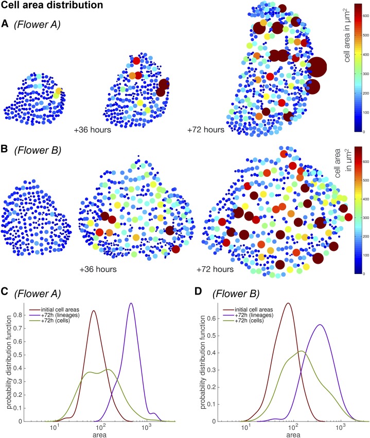
Since cell division does not have a major effect on growth, we asked if it has a role in generating cell size diversity as we have previously reported (Roeder et al., 2010). In mature sepals, epidermal cells exhibit considerable variability in size (Fig. 1, B and C). We did not observe any obvious spatial pattern in the distribution of large and small cells (Fig. 10, A and B; Supplemental Fig. S10). Large epidermal cells grew next to one another and were surrounded by small cells. We observed that the range and variability of cell areas increased over time (Fig. 10; Supplemental Fig. S10). To determine how this variability is generated, we compared the cell area distributions versus nondividing cell lineages before and after 72 h of growth. We first compared the initial distribution of cell areas with the final distribution of cell areas and observed that distribution became broader, indicating increased variability in cell area (Fig. 10, C and D, red curve versus green curve). We then considered the areas of the whole-cell lineages to determine what would have happened if the cells had not divided. The lineage area curves appeared similar to the initial cell area curves, except that they were shifted to larger sizes; the curves maintained approximately the same shape and width (Fig. 10, C and D, purple curve). This suggests that the increased variability was not due to unequal GRs of different cell lineages, but instead was mostly produced by nonuniform cell divisions within those lineages. These results are consistent with our previous analysis showing that the diversity in cell sizes correlates with variability in the time at which cells divide or enter endoreduplication (Roeder et al., 2010). Since cell division did not have a major effect on growth, we continued to focus our analysis on cell lineages.

Figure 10.

Cell size variability increases in time. A and B, The variability in cell areas increases after 36 h and further increases after 72 h compared with the initial time point for flowers A (A) and B (B). Each cell is represented as a dot whose size and color (colormap) are scaled according to the cell area. Each dot is positioned at the cell center; note that there is no obvious spatial pattern in the distribution of large and small cells. The sepal and the cell centers of each cell are flattened to two dimensions for visualization purposes. C and D, The cell area distribution curves from an initial time point (red) become broader at the final time point 72 h later (green) when cell division is taken into account for flowers A (C) and B (D). In contrast, when cell lineages are considered without cell division (blue), the curve shape is maintained and the curve is shifted to the right due to growth.

Each Cell Lineage Reaches the Same Maximum RGR

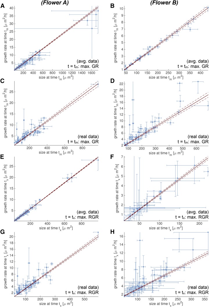
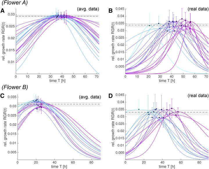
To determine whether there are similarities in the underlying growth trends between cell lineages, we analyzed the relationships between the individual best-fitting S growth curves. Cell lineages with insufficient data points (<8), without a meaningful fit to an S curve (R² < 0.9) or high uncertainty in the fitting parameters (see Supplemental Text S1 for details), were excluded from the analysis. Given these conditions, we observed a strikingly linear correlation between the GR and the cell size at time t_m, the time at which the maximal GR was reached and growth began to slow down (Fig. 11, A–D; Supplemental Fig. S11). This linear correlation suggested that all cell lineages at their time t_m have the same RGR: RGR(t_m) = GR(t_m)/area(t_m) (Table I). Furthermore, we observed a linear relationship between the GR and the cell size at time t_x, the time at which the cell lineages reached their maximal RGR(t_x) (Fig. 11, E–H; Supplemental Fig. S11). This suggests that each cell lineage reaches the same maximum RGR(t_x) (Table I). To confirm this, the RGR for each cell lineage was plotted. All cell lineages indeed reached the same maximum RGR, but each lineage reaches it at different times (Fig. 12).

Figure 11.

GR and size are linearly correlated at times t_m and t_x. We analyze growth curves for flowers A (A, C, E, and G) and B (B, D, F, and H) using both the spatially averaged (A and B, E and F) and the real (C and D, G and H) data. We consider the time point t_m (A–D) when the GR is maximal, and the time point t_x (E–H) when the RGR(t) = GR(t) / area(t) is maximal. In all cases, we observe a linear correlation between GR and size, which suggests that RGR(t_m) is the same for all cell lineages in the sepal. Likewise, this suggests that RGR(t_x) is the same for all cell lineages in the sepal (see Fig. 12). Both the GR [GR(t_m) and GR(t_x)] and the size [area(t_m) and area(t_x)] are estimated from the fit of the data to an S curve. We only consider data with a meaningful fit. The uncertainty from the fit is propagated into an Sd for GR and area, which is shown in the plots as error bars. We fit constants for RGR(t_m) and RGR(t_x) and show them as red lines, with 95% confidence bounds as dotted lines.

Table I. All cell lineages in the sepal have the same RGR at t = t_m (where GR is maximal) and the same RGR at t = t_x (where RGR is maximal).

We report the RGR (h⁻¹) with sds propagated from the uncertainty of the fit. For the average data, the constant RGR is consistently lower. This may be explained with a noisy fit for the real data. An S curve may better approximate noisy data using a more step-like shape, which essentially decreases the duration of growth and increases the GRs as observed here.

Time Point	Flower	RGR (h−1)
		Average Data	Real Data
t = tm	A	0.0234 ± 0.00021	0.0293 ± 0.000641
t = tx	A	0.0293 ± 0.000128	0.0339 ± 0.000488
t = tm	B	0.0232 ± 0.000353	0.0269 ± 0.00061
t = tx	B	0.0312 ± 0.000437	0.0331 ± 0.000602

Figure 12.

Cell lineages reach the same maximal RGR. We show the RGR(t) for flowers A (A and B) and B (C and D) obtained from the best-fitting S curve for the spatially averaged (A and C) and the real (B and D) data. The maximum RGR for each lineage is marked with a dot at RGR(t_x). The uncertainty from the fit is propagated into an sd for RGR(t_x), which is shown in the plots as error bars. Note that all cell lineages reach the same maximum RGR, although the time t_x, at which a cell reaches its maximum RGR, varies between cell lineages. The constant value for the maximum RGR(t_x) (Table I; Fig. 11, C, D, G, and H) is displayed as a dashed black line with its 95% confidence bounds as dotted lines. We only consider data with a meaningful fit. The curves are colored according to t_x (early [cyan] to late [purple]).

Variability in Cell Lineage Growth Is Mostly Due to the Timing of Maximum Growth and the Size of the Cell Lineage at That Time

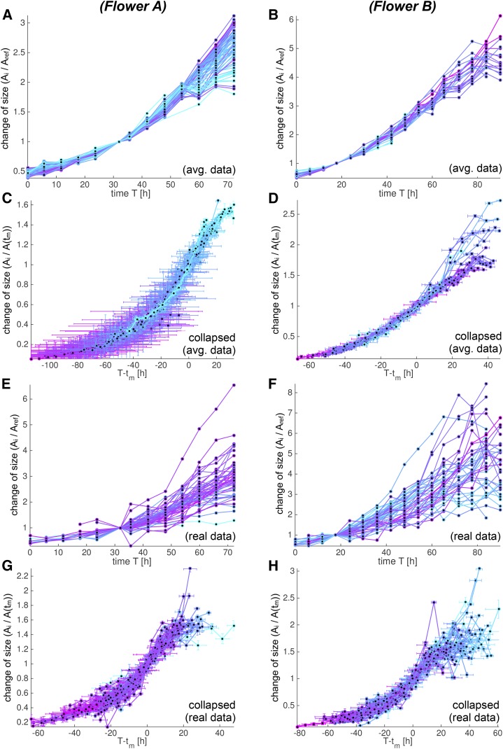
To investigate the relationships between cell lineage growth curves, we aligned the growth curves in time by removing the dependency of t_m and scaled the curves according to the lineage size at time t_m. Thus, the slope of these curves at time t_m corresponds to RGR(t_m). If the value of RGR(t_m) is the same for each cell lineage and the value of RGR(t_x) is the same for each cell lineage, then the transformed S curves should collapse into a single S curve (for details, see Supplemental Text S1). If both RGR values are different among lineages, then the transformed curves may differ between cells because each growth curve is still dependent on three of the four fitting parameters. We found that the transformed growth curves indeed collapsed onto a single S curve (Fig. 13; Supplemental Fig. S12). This confirmed that RGR(t_m) and RGR(t_x) were the same for all lineages. Furthermore, the collapse of these curves demonstrates that the time at which each cell lineage reaches t_m and the size of the cell lineage at t_m are the major sources of variability in cell lineage growth. Individual cell wall growth curves followed the same pattern as cell lineage areas (Supplemental Figs. S13 and S14).

Figure 13.

Individual growth curves can be collapsed to similar S curves. We analyze growth curves for flowers A (A, C, E, and G) and B (B, D, F, and H) using both the spatially averaged (A–D) and the real (E–H) data. The growth curves are colored according to t_m (early [cyan] to late [purple]). A, B, E, and F, The individual growth curves f(T) show the change in each cell lineage area in time compared with the reference time. The curve f(T) is only defined at discrete time points T = t_i marked with dots [f(t_i) = A_i/A_ref]. We only consider data with a meaningful fit to an S curve. C, D, G, and H, We collapsed the growth curves into more similar curves by aligning them according to the nearly constant RGR(t_m). We aligned them in time by removing the dependency of t_m, and we scaled the curves according to their size at time t_m such that their slope corresponds to RGR(t_m). We therefore computed f_c(t) = f(t + t_m)/f(t_m) and plotted f_c(t) against t = T – t_m. Both t_m and f(t_m) were estimated from the best-fitting S curve, whereas we evaluated f(t + t_m) at discrete time points t = t_i – t_m from the actual data [f_c(t_i − t_m) = A_i/A(t_m)]. Note that since f still depends on three of the four parameters defining the S curve, it was not obvious the curves would collapse to a single curve. The fact that the transformed growth curves f_c(t) lined up well confirmed that the RGRs at times t_m and t_x were the same for each cell lineage.

Spatial Trends in Growth

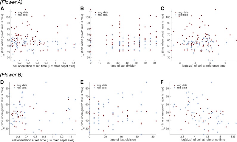
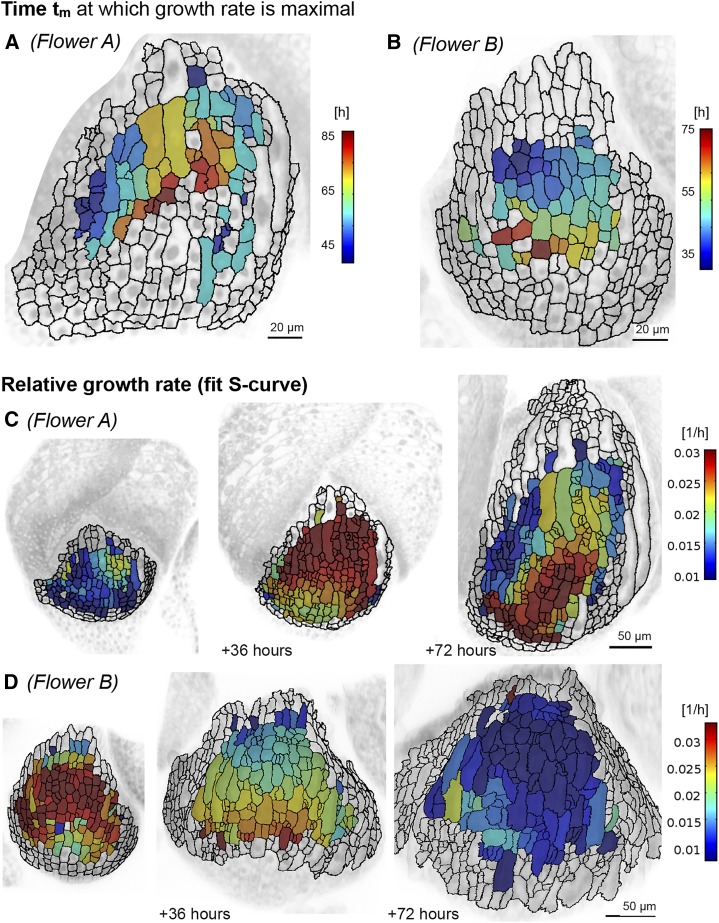
Our previous analysis indicated that the time t_m at which the maximum GR is reached is one of the major sources of variation between cell lineages. We therefore looked for correlations of t_m with other properties of the sepal (Fig. 14; Supplemental Figs. S15 and S16). For instance, cells elongated along the main sepal axis might be expected to have different growth timings. Yet, we found that there was no obvious correlation between t_m and the cell orientation within the sepal (Fig. 14, A and D; Supplemental Figs. S15 and S16). Likewise, we hypothesized that growth might correlate with the cell cycle type, whether mitotic division or endoreduplication. However, we found that there was no obvious correlation between t_m and the type of cell cycle as determined by the time of the last observed division (cells that divided toward the end of the time series were in mitosis, whereas those that never divided or divided only at the start of the time series were likely to be endoreduplicating; Fig. 14, B and E; Supplemental Figs. S15 and S16). Thus, endoreduplication does not appear to have a major effect on the cellular growth parameters. Finally, we saw no correlation between t_m and the cell area at the reference time point (Fig. 14, C and F; Supplemental Figs. S15 and S16), suggesting that the time point when cell growth slows down does not depend on the cell size at a fixed time t. However, t_m followed a smooth spatial distribution with an apical to basal trend; cells in the top of the sepal tended to reach t_m earlier than those further down the sepal (Fig. 15, A and B; Supplemental Fig. S17).

Figure 14.

T_m does not correlate with cell orientation, time of last division, or area. We looked for correlations between t_m and cell orientation (A and D), time of last division (B and E), and ln(area) (C and F) for real (blue) and spatially averaged (red) cell lineages of flowers A (A–C) and B (D–F). The cell orientation is measured as the angle (radians) between the main sepal axis and the main axis of each cell. The time of last division is indicative of whether the cell lineage is actively dividing (late time of last division) or endoreduplicating (early time of last division). We take the logarithm of the cell area to avoid spreading out. Both the area and the angle are measured at the reference time point.

Figure 15.

We observe spatial trends for the RGR and the time of maximum growth. A and B, Spatial distribution of t_m appears smooth, with a trend from the top to the bottom of the sepal for flowers A (A) and B (B). We only consider data with a meaningful fit to a S function. The data are shown on the mesh at t = t_r. Scale = 20 μm. C and D, The RGR(t) of flowers A (C) and B (D) at an initial time point and 36 and 72 h later. We show RGR(t) based on the fit to an S curve. Note that, whereas individual neighbors can have different RGRs, there is a peak of faster growth that starts at the tip of the sepal and moves downward as the sepal develops. Scale = 50 μm.

Although our data suggest that all cells reach the same maximum RGR(t_x), each cell reaches this maximum at a different time. Each cell and each wall segment had a different value for t_m, which shifted the S curve in time (Fig. 15, A and B; Supplemental Fig. S17). Thus, at a single time point in the developmental series, cells have different RGR(t). We evaluated RGR(t) based on the fit to an S curve (Fig. 15, C and D; Supplemental Videos S7 and S8; Supplemental Fig. S17), which resulted in a smooth distribution of RGR(t) in comparison with our initial analysis of the RGR (Figs. 3 and 4; Supplemental Figs. S3 and S4). We observed that cells at the top of the sepal reached a high RGR first, and this high RGR subsequently moved down the sepal. Thus, both t_m and the maximum RGR show a spatial gradient progressing from top to bottom as the sepal develops.

DISCUSSION

We have quantified the growth of cell lineages in the Arabidopsis sepal. Our results reveal that sepal cell lineages all follow the same growth curve, but that curve is shifted in time and scaled by size, creating the heterogeneity in GRs observed at a single time (t) in a tissue. Using spatially averaged, smooth displacement fields, we were able to capture the cellular kinematics in the sepal and provide a consistent smoothing of the experimental data. We extracted growth curves for individual cell areas and wall segment lengths as well as the tissue. We found that the growth of the tissue, the cell lineage areas, and the length of individual cell walls fit S curves, indicating that the GRs change in time. Within the S curves, we observed a striking linear relationship between the GR and the size of cells and walls at the time of maximal GR (t_m) and at the time of maximal RGR (i.e. GR divided by area; t_x). We found that all cell lineages reach the same maximum RGR(t_x). However, the time at which each lineage reaches this maximum RGR is different within the development of the sepal, accounting for the variability of growth observed.

Our analysis showed that the growth of tissues, cell lineages, and walls best fit S curves. For the parameter ranges observed in our fits, the RGR(t) plotted against time was a bell-shaped curve (Fig. 12). This meant that, within a single cell lineage, RGR(t) was small at early time points, increased until it reached its maximal value at t = t_x, and then decreased again afterward. Similarly, studies that measured the full organ growth reported size increases consistent with a S curve (De Veylder et al., 2001; Mündermann et al., 2005; Kuchen et al., 2012; Remmler and Rolland-Lagan, 2012; Rolland-Lagan et al., 2014). For instance, Mündermann et al. (2005) measured the width of sepals and reported fits to a S curve, consistent with our results. They also observed S curves for the growth of leaves, petals, anthers, carpels, pedicels, and filaments (Mündermann et al., 2005). In contrast, the growth in size of individual bacteria or fission yeast cells have been shown to fit bilinear curves (Reshes et al., 2008; Baumgärtner and Tolić-Nørrelykke, 2009).

It is common in the analysis of plant cell growth to implicitly assume exponential growth. Plant cell growth is often modeled with Lockhart's equations or variants thereof, which relate cell expansion to water uptake and turgor pressure (Lockhart, 1965; Cosgrove, 1986). Given a constant turgor pressure, a constant yield stress for the cell walls, and a comparably fast water uptake, Lockhart's equations predict a constant RGR, which leads to exponential growth. An S curve, such as the ones observed in sepal growth, may be approximated with an exponential curve at early times, but at intermediate and late times, a flattening of the GRs is observed that cannot be captured by an exponential. To explain the S curve with Lockhart’s equation, RGR(t) can vary in time if the cell wall’s extensibility φ or the difference in water potential ∆Ψ are a function of time. Lockhart envisioned that φ(t) → 0 and ∆Ψ(t) → 0 may be two mechanisms to slow down the growth of cylindrical plant cells that eventually reach maturity (Lockhart, 1965). Thus, it is not surprising to see S curves when analyzing real growth curves. A decreasing wall extensibility φ may be obtained by strain stiffening (Kierzkowski et al., 2012), wall hardening (Huang et al., 2012), or by having a thicker cell wall (Schopfer, 2006). In future studies, it will be interesting to use the results of our study to validate numerical models (Dupuy et al., 2010; Koumoutsakos et al., 2011; Huang et al., 2012; Kierzkowski et al., 2012; Fozard et al., 2013) within a Bayesian uncertainty quantification and propagation framework (Angelikopoulos et al., 2012). Such a framework would be able to quantify which model is most probable given the data.

The striking similarity in the shape of the sepal cell lineage growth curves and the finding that all cell lineages reach the same maximum RGR have, to our knowledge, not been observed previously. These finding suggest a common underlying growth curve. How can this underlying similarity be explained? The similarity could imply that there is global coordination between cells within the growing tissue, or intrinsic constraints due to gene regulation or mechanical properties of the walls. Although we do see differences between neighboring cells, overall, our analysis shows that the growth of cells in the sepal is less heterogeneous than it initially appears. The initial appearance of growth heterogeneity observed in our results (Fig. 3) and others’ results can be explained by shifting the S curves of each cell lineage in time. At a single time point, one cell lineage may be in the initial part of the S curve where its RGR is low, whereas its neighbor may be at the point of the sigmoid curve where its RGR is at the maximum. At a single time point, cell lineages will have different RGRs, whereas if we observed each cell lineage when the RGR is at the maximum, they would have the same RGR. Thus, neighboring cells are simply at different stages of growth and consequently have different RGRs at a single time point.

Most of the variability in the growth of cell lineages is in the time t_m, when the GR reaches its maximum and starts to slow down, and the size of the cell lineage at t_m. Our analysis revealed a smooth spatial distribution of t_m. There is an apical to basal trend in t_m, which parallels the development of the sepal (Donnelly et al., 1999; Roeder et al., 2010; Andriankaja et al., 2012). Cells at the top of the sepal are generated first, and consequently mature first, reaching t_m earlier in development. Simultaneously, new cells are constantly generated at the base of the sepal, and these cells subsequently mature, reaching t_m later in development of the sepal. This explains why cells in the tip of the sepal also reach the maximum RGR earlier than cells lower in the sepal. However, the apical basal gradient does not explain all of the variation in t_m, so it will be interesting to identify other factors influencing t_m in the future.

The use of continuous low-order displacement fields enabled the filtering of spatial differences as well as segmentation noise to capture the similarities and differences in the growth curves of sepal cell lineages. Any image-processing analysis is subject to errors from segmentation noise, and such tools can help alleviate this issue. Real spatial differences between cells may be of interest biologically, and what we classify as noise may be important subtle patterns in the growth (e.g. fractals), but this hides broader trends. The spatially averaged data from the low-order displacement field allowed us to detect hidden similarities in growth curves that were subsequently verified in the real data. We believe this method will be useful for finding general growth trends for other plant tissues. It will be informative to determine whether leaf cell lineages in Arabidopsis and other species also all have the same maximum RGR and follow similar S curves that are shifted in time and scaled by size. Furthermore, this approach can be applied to animal tissues in which the cells do not migrate relative to one another (i.e. the bending of epithelial sheets during morphogenesis; Martin et al., 2009). A displacement field could be fitted to epithelial cells that are tightly bound to their neighbors through junctional complexes; epithelial cell migration is limited during many developmental processes, with the notable exceptions of epithelial to mesenchyme transition and convergent extension (Lim and Thiery, 2012). In addition, the displacement fields could directly be used to drive growth in simulation models or to facilitate the comparison of different samples.

Our results raise important questions for future investigations of growth. Is there a link between reproducibility of organ size and the observation that all cells reach the same maximum RGR? Does this imply that there is global coordination occurring between the cells, or that there is intrinsic constraint on the growth of each cell that leads to this regularity? Isolation of mutants disrupting the cellular or organ regularity will be key to uncovering the underlying mechanism.

MATERIALS AND METHODS

Plant Material, Growth Conditions, and Image Acquisition

Growth and imaging of living Arabidopsis (Arabidopsis thaliana) sepals from the Landsberg erecta accession were conducted as described previously (Roeder et al., 2010; Cunha et al., 2012; see Supplemental Text S1 for details). Individual flowers from different plants imaged in the first session were given identifiers A and D, whereas flowers imaged in a second session were given identifiers B and C. Flower A was imaged for 72 h, flower B for 90 h, flower C for 102 h, and flower D for 66 h. The division pattern of the cells for flowers A and D have been previously analyzed (Roeder et al., 2010). Results for flowers C and D are presented in Supplemental Figures S1, S3 to S7, S9 to S12, S16, and S17.

To define similar initial time points for the flowers (Fig. 2), we manually aligned the fluorescent stacks of flowers A and B such that they looked similar in size and shape (Supplemental Fig. S18). We observed that, 72 h after the chosen initial time point, the sepals were similar in length, but flower B was wider. Most likely, this was because we looked at a lateral sepal for flower A, which was partly being masked by other overlying sepals.

We compared the size of the sepals with the staging of Smyth et al. (1990) by considering the sepal height. We observed that flower A was in stages 8 and 9, flower B was in stages 7 to 9, flower C was in stages 8 and 9, and flower D was in earlier stages 4 to 8. We note that at those stages, guard cells have not fully developed, but giant cells are forming. We also considered the sepal width and compared with the data analyzed by Mündermann et al. (2005). We estimated that their analysis started right after our data sets end for flowers A, B, and C.

Image Processing

We analyzed the growth of the sepals with an extended version of the MorphoGraphX image analysis software (Supplemental Fig. S2; Supplemental Videos S1 and S2; Kierzkowski et al., 2012; Barbier de Reuille et al., 2015). We constructed a curved surface mesh on top of the sepal by extracting an isosurface of the propidium iodide-stained stack using a marching-cubes algorithm. The mesh was further smoothened and refined to contain approximately 1,000 vertices per cell. We then projected the intensities of the fluorescent nuclei and membrane markers from the stack (in a band 1–6 µm away from the surface) onto the surface mesh. The surface mesh was then segmented into cells using a watershed method. All polygons belonging to a cell were marked with the same label. The areas of the polygons belonging to the same cell were summed up to compute the cell area while taking into account the curvature of the surface. The length of each cell wall segment was estimated by fitting a quadratic function to the border vertices. This avoided errors due to the zig-zag shape that would have appeared when following the border vertices (see Supplemental Text S1 for details). The signal at the border of the sepal was noisier due to the reduced resolution in the z-direction for confocal microscopy and the curvature of the sepal. We therefore removed cells and walls next to the border from the analysis.

To analyze growth, we have developed and used a new tool for tracking cell lineages in MorphoGraphX (Barbier de Reuille et al., 2015). Each cell was mapped, if possible, to its equivalent or its parent cell in the segmented mesh of the previous time point. Due to imaging noise and imperfect microscopy conditions, not all cells were segmented in each time point. Each newly appearing cell was assigned a unique label, and its area was tracked over several time points until the cell or one of its daughter cells disappeared from the segmentation. The area of a cell lineage was computed by summing up the daughter cells' areas. We also tracked each wall segment by considering the lineage of its neighboring cells.

To estimate segmentation errors in the image processing, we independently reanalyzed three time points of flower D (Supplemental Fig. S19) and observed that cell areas varied by 20% between independent segmentations. We therefore expected segmentation errors to be of a similar size, approximately 20%, for all data sets. We hence assumed that such errors would affect an analysis of broader spatial growth trends unless a spatial averaging was performed.

Continuous Low-Order Displacement Fields

We used the tracking of cells and wall segments to define continuous low-order displacement fields u(X, t_j) between a reference time point t_ref and any other time point t_j. We considered the centers of each cell and wall segment shared between the time points t_j and t_ref as landmark points. We did not consider dividing cells and walls because we had enough shared points without them. We used the center of each wall segment as opposed to the junctions between wall segments because segmentation errors were larger for junctions.

Each landmark point i had a three-dimensional position X_i at time t_ref and x_ij at time t_j. We then identified the best-fitting low-order function u(X, t_j) by minimizing the sum of squared errors [x_ij – X_i – u(X_i, t_j)]² over all landmark points i. The reference time t_ref was the time point that contained the most shared landmarks between the live-imaging series. Given u(X, t_j), we estimated spatially averaged displacements in the sepal as well as the deformation of line elements and area elements (see Supplemental Text S1 for details).

We fit each dimension of u(X, t_j) separately with a robust linear regression routine in MATLAB (LinearModel.fit; MathWorks) using an iteratively reweighted least-squares method with a bisquare weighting function. We automatically selected the best-fitting model among linear, quadratic, and cubic models using the Akaike information criterion corrected (AICc) for small sample sizes, which penalizes for overfitting (Burnham and Anderson, 2002).

Growth Rates and Growth Curves

We denote the time evolution of the area of a cell or the length of a wall segment as f(t), and define the GR(t) as the slope of f(t) [GR(t) = df(t)/dt] and the RGR as RGR(t) = GR(t)/f(t). If f(t) is only known at discrete time points t_i, we can estimate an average RGR by computing RGR_i = ln(f_i+1/f_i)/(t_i+1 − t_i), where f_i = f(t_i) (Figs. 3 and 4).

We reported the increase in areas A_i and lengths L_i at time t_i with respect to the reference time t_ref as A_i/A_ref and L_i/L_ref, respectively, as growth curves. To compare growth curves, we defined statistics based on fitting an S curve (Fig. 8C). We used a shifted logistic function with four parameters (a, b, k, t_m) defined as

The function fitting was performed by minimizing the sum of squared errors within a constrained optimization routine in MATLAB (fmincon) with {a,b,k} ≥ 0. We repeated the optimization with an exponential [f(t) = a exp(k t)] and a linear [f(t) = a t + b] function. Given the results of the optimizations, we computed the AICc for each function (see Supplemental Text S1 for details). The AICc considers the sum of squared errors as well as the number of parameters of the fit and hence penalizes for overfitting. The functions were ranked according to their AICc (AIC_i), with the best function being the one with the minimal AICc (AIC_min). The relative probabilities of each considered function were then computed as exp[(AIC_min – AIC_i)/2] and subsequently normalized to define the probability of each function (Burnham and Anderson, 2002).

The parameters of the S curve f(t) can be interpreted as b being the lower plateau of the curve, a+b being the upper plateau, k defining the steepness of the curve, and t_m being the time when the GR(t) is maximal (Fig. 8C). Given these parameters, we can furthermore compute the time t_x = t_m − ln[(a+b)/b]/(2 k), where the RGR(t) is maximal (see Supplemental Text S1 for details).

We expected our data to have unknown measurement and segmentation errors, and we did not assume that the S curve was the perfect model for the growth curves but merely an approximation. These three factors led to uncertainties in the fitting parameters (a, b, k, t_m). We used those uncertainties to distinguish meaningful growth parameters. We furthermore propagated the uncertainties to derived quantities such as f(t), GR(t), RGR(t), and t_x. The uncertainties were translated to standard deviations and reported either as error bars or as 95% confidence intervals (see Supplemental Text S1 for details). MATLAB code and data used for the analysis are in Supplemental Code S1.

Supplemental Data

The following supplemental materials are available.

• Supplemental Figure S1. Cell lineage tracking in live images of growing Arabidopsis sepals.

• Supplemental Figure S2. Image-processing workflow.

• Supplemental Figure S3. The RGR is noisy.

• Supplemental Figure S4. A low-order displacement field smoothens growth.

• Supplemental Figure S5. Spatially averaged kinematics fit the real data well.

• Supplemental Figure S6. Uniform growth in space predicts cellular growth.

• Supplemental Figure S7. Tissue growth curves fit S shapes.

• Supplemental Figure S8. Individual wall segment growth curves fit S shapes.

• Supplemental Figure S9. Individual cell lineage growth curves fit S shapes.

• Supplemental Figure S10. Cell size variability increases in time.

• Supplemental Figure S11. GR and size are linearly correlated at times t_m and t_x.

• Supplemental Figure S12. Individual growth curves can be collapsed to similar S curves.

• Supplemental Figure S13. GR and size of wall segments are linearly correlated at times t_m and t_x.

• Supplemental Figure S14. Individual growth curves of wall segments can be collapsed to similar S curves.

• Supplemental Figure S15. T_m of wall segments does not correlate with wall orientation, time of last division, or length.

• Supplemental Figure S16. T_m does not correlate with cell orientation, time of last division, or area.

• Supplemental Figure S17. We observe spatial trends for the RGR and the time of maximum growth.

• Supplemental Figure S18. Comparison of sepals.

• Supplemental Figure S19. Estimation of segmentation error.

• Supplemental Text S1. Supplemental materials and methods.

• Supplemental Video S1. Cell lineage tracking for flower A (as in Fig. 2A).

• Supplemental Video S2. Cell lineage tracking for flower B (as in Fig. 2B).

• Supplemental Video S3. RGR estimated from live-imaging data for flower A (as in Fig. 3A).

• Supplemental Video S4. RGR estimated from live-imaging data for flower B (as in Fig. 3B).

• Supplemental Video S5. RGR estimated from spatially averaged data for flower A (as in Fig. 4A).

• Supplemental Video S6. RGR estimated from spatially averaged data for flower B (as in Fig. 4B).

• Supplemental Video S7. RGR estimated after fitting an S curve to the spatially averaged data for flower A (as in Fig. 15C).

• Supplemental Video S8. RGR estimated after fitting an S curve to the spatially averaged data for flower B (as in Fig. 15D).

• Supplemental Code S1. MATLAB code and data used for the analysis in this work.

Glossary

S

sigmoid

RMSE

root mean squared error

GR

growth rate

RGR

relative growth rate

References

- Andriankaja M, Dhondt S, De Bodt S, Vanhaeren H, Coppens F, De Milde L, Mühlenbock P, Skirycz A, Gonzalez N, Beemster GTS, et al. (2012) Exit from proliferation during leaf development in Arabidopsis thaliana: a not-so-gradual process. Dev Cell 22: 64–78 [DOI] [PubMed] [Google Scholar]
- Angelikopoulos P, Papadimitriou C, Koumoutsakos P (2012) Bayesian uncertainty quantification and propagation in molecular dynamics simulations: a high performance computing framework. J Chem Phys 137: 144103. [DOI] [PubMed] [Google Scholar]
- Asl LK, Dhondt S, Boudolf V, Beemster GTS, Beeckman T, Inzé D, Govaerts W, De Veylder L (2011) Model-based analysis of Arabidopsis leaf epidermal cells reveals distinct division and expansion patterns for pavement and guard cells. Plant Physiol 156: 2172–2183 [DOI] [PMC free article] [PubMed] [Google Scholar]
- Barbier de Reuille P, Routier-Kierzkowska A-L, Kierzkowski D, Bassel GW, Schüpbach T, Tauriello G, Bajpai N, Strauss S, Weber A, Kiss A, et al. (2015) MorphoGraphX: A platform for quantifying morphogenesis in 4D. eLife 4: 05864. [DOI] [PMC free article] [PubMed] [Google Scholar]
- Baumgärtner S, Tolić-Nørrelykke IM (2009) Growth pattern of single fission yeast cells is bilinear and depends on temperature and DNA synthesis. Biophys J 96: 4336–4347 [DOI] [PMC free article] [PubMed] [Google Scholar]
- Besson S, Dumais J (2011) Universal rule for the symmetric division of plant cells. Proc Natl Acad Sci USA 108: 6294–6299 [DOI] [PMC free article] [PubMed] [Google Scholar]
- Burnham KP, Anderson DR (2002) Model selection and multimodel inference: A practical information-theoretic approach, 2nd ed. Springer, New York: doi: 10.1007/b97636 [Google Scholar]
- Cosgrove D. (1986) Biophysical control of plant cell growth. Annu Rev Plant Physiol 37: 377–405 [DOI] [PubMed] [Google Scholar]
- Cosgrove DJ. (2005) Growth of the plant cell wall. Nat Rev Mol Cell Biol 6: 850–861 [DOI] [PubMed] [Google Scholar]
- Cunha A, Tarr PT, Roeder AHK, Altinok A, Mjolsness E, Meyerowitz EM (2012) Computational analysis of live cell images of the Arabidopsis thaliana plant. Methods Cell Biol 110: 285–323 [DOI] [PubMed] [Google Scholar]
- De Veylder L, Beeckman T, Beemster GT, Krols L, Terras F, Landrieu I, van der Schueren E, Maes S, Naudts M, Inzé D (2001) Functional analysis of cyclin-dependent kinase inhibitors of Arabidopsis. Plant Cell 13: 1653–1668 [DOI] [PMC free article] [PubMed] [Google Scholar]
- Donnelly PM, Bonetta D, Tsukaya H, Dengler RE, Dengler NG (1999) Cell cycling and cell enlargement in developing leaves of Arabidopsis. Dev Biol 215: 407–419 [DOI] [PubMed] [Google Scholar]
- Dupuy L, Mackenzie J, Haseloff J (2010) Coordination of plant cell division and expansion in a simple morphogenetic system. Proc Natl Acad Sci USA 107: 2711–2716 [DOI] [PMC free article] [PubMed] [Google Scholar]
- Elsner J, Michalski M, Kwiatkowska D (2012) Spatiotemporal variation of leaf epidermal cell growth: a quantitative analysis of Arabidopsis thaliana wild-type and triple cyclinD3 mutant plants. Ann Bot (Lond) 109: 897–910 [DOI] [PMC free article] [PubMed] [Google Scholar]
- Fozard JA, Lucas M, King JR, Jensen OE (2013) Vertex-element models for anisotropic growth of elongated plant organs. Front Plant Sci 4: 233. [DOI] [PMC free article] [PubMed] [Google Scholar]
- Hamant O, Heisler MG, Jönsson H, Krupinski P, Uyttewaal M, Bokov P, Corson F, Sahlin P, Boudaoud A, Meyerowitz EM, et al. (2008) Developmental patterning by mechanical signals in Arabidopsis. Science 322: 1650–1655 [DOI] [PubMed] [Google Scholar]
- Huang R, Becker AA, Jones IA (2012) Modelling cell wall growth using a fibre-reinforced hyperelastic-viscoplastic constitutive law. J Mech Phys Solids 60: 750–783 [Google Scholar]
- Kaplan DR, Hagemann W (1991) The relationship of cell and organism in vascular plants: Are cells the building-blocks of plant form. Bioscience 41: 693–703 [Google Scholar]
- Kierzkowski D, Nakayama N, Routier-Kierzkowska A-L, Weber A, Bayer E, Schorderet M, Reinhardt D, Kuhlemeier C, Smith RS (2012) Elastic domains regulate growth and organogenesis in the plant shoot apical meristem. Science 335: 1096–1099 [DOI] [PubMed] [Google Scholar]
- Koumoutsakos P, Bayati B, Milde F, Tauriello G (2011) Particel simulations of morphogenesis. Math Models Methods Appl Sci 21: 955–1006 [Google Scholar]
- Kuchen EE, Fox S, de Reuille PB, Kennaway R, Bensmihen S, Avondo J, Calder GM, Southam P, Robinson S, Bangham A, et al. (2012) Generation of leaf shape through early patterns of growth and tissue polarity. Science 335: 1092–1096 [DOI] [PubMed] [Google Scholar]
- Lim J, Thiery JP (2012) Epithelial-mesenchymal transitions: insights from development. Development 139: 3471–3486 [DOI] [PubMed] [Google Scholar]
- Lockhart JA. (1965) An analysis of irreversible plant cell elongation. J Theor Biol 8: 264–275 [DOI] [PubMed] [Google Scholar]
- Martin AC, Kaschube M, Wieschaus EF (2009) Pulsed contractions of an actin-myosin network drive apical constriction. Nature 457: 495–499 [DOI] [PMC free article] [PubMed] [Google Scholar]
- Meyer HM, Roeder AHK (2014) Stochasticity in plant cellular growth and patterning. Front Plant Sci 5: 420. [DOI] [PMC free article] [PubMed] [Google Scholar]
- Mündermann L, Erasmus Y, Lane B, Coen E, Prusinkiewicz P (2005) Quantitative modeling of Arabidopsis development. Plant Physiol 139: 960–968 [DOI] [PMC free article] [PubMed] [Google Scholar]
- Poethig RS, Sussex IM (1985) The cellular parameters of leaf development in tobacco: a clonal analysis. Planta 165: 170–184 [DOI] [PubMed] [Google Scholar]
- Qu X, Chatty PR, Roeder AHK (2014) Endomembrane trafficking protein SEC24A regulates cell size patterning in Arabidopsis. Plant Physiol 166: 1877–1890 [DOI] [PMC free article] [PubMed] [Google Scholar]
- Reddy GV, Heisler MG, Ehrhardt DW, Meyerowitz EM (2004) Real-time lineage analysis reveals oriented cell divisions associated with morphogenesis at the shoot apex of Arabidopsis thaliana. Development 131: 4225–4237 [DOI] [PubMed] [Google Scholar]
- Remmler L, Rolland-Lagan A-G (2012) Computational method for quantifying growth patterns at the adaxial leaf surface in three dimensions. Plant Physiol 159: 27–39 [DOI] [PMC free article] [PubMed] [Google Scholar]
- Reshes G, Vanounou S, Fishov I, Feingold M (2008) Cell shape dynamics in Escherichia coli. Biophys J 94: 251–264 [DOI] [PMC free article] [PubMed] [Google Scholar]
- Roeder AHK. (2012) When and where plant cells divide: a perspective from computational modeling. Curr Opin Plant Biol 15: 638–644 [DOI] [PubMed] [Google Scholar]
- Roeder AHK, Chickarmane V, Cunha A, Obara B, Manjunath BS, Meyerowitz EM (2010) Variability in the control of cell division underlies sepal epidermal patterning in Arabidopsis thaliana. PLoS Biol 8: e1000367. [DOI] [PMC free article] [PubMed] [Google Scholar]
- Roeder AHK, Cunha A, Ohno CK, Meyerowitz EM (2012) Cell cycle regulates cell type in the Arabidopsis sepal. Development 139: 4416–4427 [DOI] [PubMed] [Google Scholar]
- Roeder AHK, Tarr PT, Tobin C, Zhang X, Chickarmane V, Cunha A, Meyerowitz EM (2011) Computational morphodynamics of plants: integrating development over space and time. Nat Rev Mol Cell Biol 12: 265–273 [DOI] [PMC free article] [PubMed] [Google Scholar]
- Rolland-Lagan AG, Coen E, Impey SJ, Bangham JA (2005) A computational method for inferring growth parameters and shape changes during development based on clonal analysis. J Theor Biol 232: 157–177 [DOI] [PubMed] [Google Scholar]
- Rolland-Lagan AG, Remmler L, Girard-Bock C (2014) Quantifying shape changes and tissue deformation in leaf development. Plant Physiol 165: 496–505 [DOI] [PMC free article] [PubMed] [Google Scholar]
- Sampathkumar A, Krupinski P, Wightman R, Milani P, Berquand A, Boudaoud A, Hamant O, Jönsson H, Meyerowitz EM (2014) Subcellular and supracellular mechanical stress prescribes cytoskeleton behavior in Arabidopsis cotyledon pavement cells. eLife 3: e01967. [DOI] [PMC free article] [PubMed] [Google Scholar]
- Schopfer P. (2006) Biomechanics of plant growth. Am J Bot 93: 1415–1425 [DOI] [PubMed] [Google Scholar]
- Smyth DR, Bowman JL, Meyerowitz EM (1990) Early flower development in Arabidopsis. Plant Cell 2: 755–767 [DOI] [PMC free article] [PubMed] [Google Scholar]
- Somerville C, Bauer S, Brininstool G, Facette M, Hamann T, Milne J, Osborne E, Paredez A, Persson S, Raab T, et al. (2004) Toward a systems approach to understanding plant cell walls. Science 306: 2206–2211 [DOI] [PubMed] [Google Scholar]
- Uyttewaal M, Burian A, Alim K, Landrein B, Borowska-Wykręt D, Dedieu A, Peaucelle A, Ludynia M, Traas J, Boudaoud A, et al. (2012) Mechanical stress acts via katanin to amplify differences in growth rate between adjacent cells in Arabidopsis. Cell 149: 439–451 [DOI] [PubMed] [Google Scholar]
- Zhang C, Halsey LE, Szymanski DB (2011) The development and geometry of shape change in Arabidopsis thaliana cotyledon pavement cells. BMC Plant Biol 11: 27. [DOI] [PMC free article] [PubMed] [Google Scholar]
Associated Data
This section collects any data citations, data availability statements, or supplementary materials included in this article.