Electrospray Mass Spectrometry for Quantitative Plasma Proteome Analysis

Summary

Electrospray ionization mass spectrometry (ESI-MS) is an efficient soft ionization procedure for macro biomolecules. However, it is a rather delicate process to produce charged molecules for mass-to-charge ratio (m/z) based measurement. In this chapter, the mechanism of ESI is briefly presented, and the experimental pipeline for quantitative profiling of plasma proteins (prefractionation immunodepletion, protein isotope tagging, 2D-HPLC separation of intact proteins, and LC-MS) is presented as applied by our group in studies of cancer biomarker discovery.

1. Introduction

Since the development of soft ionization techniques, referred to as electrospray ionization mass spectrometry (ESI-MS), in late-1980s (1), biological mass spectrometry has become of widespread use in proteomics. The measurement of the molecular weight of intact molecules, the determination of amino acid sequences, and the elucidation of the modified structures of peptides and proteins have become fairly robust procedures. The electrospray ionization process can be simply described as follows: The analyte solution is pumped through a needle to which a high voltage is applied. A Taylor cone with an excess of charge on its surface forms as a result of the electric field gradient between the ESI needle and the counter-electrode. When the solution that comprises the Taylor cone reaches the Rayleigh limit, the point at which Coulombic repulsion of the surface charge is equal to the surface tension of the solution, the droplets that contain an excess of charge detach from its tip (2). These droplets evaporate as they move toward the entrance to the mass spectrometer to produce free, charged analyte molecules that can be analyzed for their mass-to-charge ratio. There are two major mechanisms (Coulomb fission mechanism and ion evaporation mechanism) that depict the formation of the charged analyte molecules. The Coulomb fission mechanism assumes that the increased charge density due to solvent evaporation causes large droplets to divide into smaller and smaller droplets, which eventually consist only of single ions (3). The ion evaporation mechanism, which assumes the increased charge density that results from solvent evaporation, causes Coulombic repulsion to overcome the liquid's surface tension, resulting in a release of ions from droplet surfaces (4). The ESI process takes place at atmospheric pressure and generates vapor phase ions that can be analyzed for mass-to-charge ratio within the mass spectrometer. Since ESI is a gentle process without significant fragmentation of analyte ions in the gas phase, it presents two advantages for proteomics. One is MS (based on the m/z of precursor) based quantification for profiling differential expression of proteins in biological samples, and the other is sequence prediction by using an enzyme that cleaves proteins at particular residues (i.e., trypsin) for peptide identification. The introduction of nano-flow (<500 nL/min) ESI has played an important role in MS-based proteomics studies, as this made analysis of minute amounts of sample feasible without compromising on signal intensity (5). Moreover, nano-flow ESI generates smaller droplets, which makes the desolvation process more efficient.

Comprehensive profiling of the biofluid proteome has substantial relevance to the identification of circulating protein biomarkers that may have predictive value and utility for disease diagnosis and management. However, the extreme complexity and vast dynamic range of protein abundance in biological fluids, notably plasma, present a substantial challenge for comprehensive protein analysis. The dynamic range of plasma protein abundance spans at least 12 orders of magnitude. We have implemented an orthogonal multidimensional intact-protein analysis system (IPAS), coupled with protein tagging and immunodepletion of abundant proteins, to quantitatively profile the human plasma proteome (6). The strength of the intact-protein-based multidimensional separation is its ability to resolve related proteins, such as differentially modified forms, and to reduce the complexity of samples generated for mass spectrometry analysis (7). Our experimental pipeline is illustrated in Fig. 1. Briefly, following the immunodepletion (to remove the high abundance proteins), plasma proteins in each of the samples are concentrated and labeled with different tags, i.e., the isobaric 4-plex iTRAQ labeling for four different types of samples, or the isotopic 2-plex acrylamide labeling for two different types of samples (8). A mixture consisting of each of the intact-protein labeled samples is subjected to an orthogonal two-dimensional HPLC separation based on charge and hydrophobicity. Protein fractions from 2D-HPLC are dried by freeze-drying, followed by in-solution trypsin digestion. Then, the digests are subjected to LC-MS/ MS analysis. Quantification is achieved by comparing the signal intensities of identified peptides in different samples (MS for the acrylamide labeling approach and MS/MS for the iTRAQ labeling approach). We have applied our current intact-protein-based multidimensional sample preparation approach with nano-LC ESI mass spectrometry to different types of cancers for which serum and plasma were analyzed disease study with the ultimate goal of discovering. In general, we have identified ∼1,500 proteins with high confidence and obtained quantitative data for some 40% of identified proteins in a given experiment.

Fig. 1.

Pipeline of nano-LC ESI-MS analysis-based quantitative plasma proteome.

2. Materials

2.1. Sample

Samples (disease or control) are from individual subjects or pools. The protocol described here is designed for a total of 600 μL each of disease and control samples.

2.2. iTRAQ Labeling

1. Centricon YM-3 devices (millipore).

2. Exchange Buffer: 6.6 M Urea + 0.5 M TEAB (from the kit) +0.2% OG, pH 8.3.

3. Labeling buffer: 0.5 M TEAB (from the kit) +0.2% OG, pH 8.3.

4. Reduction solution: TCEP (50 mM) in the kit and ready to use.

5. Alkylation solution: iodoacetamide (200 mM), needs to be freshly prepared with water (74 mg/2 mL).

6. iTRAQ solvent: ETOH in the kit.

7. iTRAQ labeling reagent (reporter ion): 114, 115, 116, and 117 in the kit.

2.3. Acrylamide Isotope Labeling

1. Centricon YM-3 devices (millipore).

2. Labeling buffer: 8 M urea, 100 mM Tris pH 8.5, 0.5% OG (octyl-β-d-glucopyranoside).

3. Dithiothreitol (DTT): (ultrapure, USB).

4. Light acrylamide: acrylamide (>99.5% purity, Fluka).

5. Heavy acrylamide: 1,2,3–¹³C₃-acrylamide (>98% purity, Cambridge Isotope Laboratories, Andover, MA).

2.4. Protein Fractionation

2.4.1. Automated 1D-HPLC System

1D-HPLC system (Shimadzu Corporation, Columbia, MD) For immunodepletion, and the system consists of:

1. Pump System: two LC-10Ai pumps.

2. Degasser: DGU-20A3 Prominence Degasser.

3. Column oven: CTO-20 Prominence Column Oven.

4. Detector: SPD-20 UV/VIS Prominence Detector.

5. 5 Collector: FRC-10A Fraction Collector.

6. Controller: SCL-10A VP System Controller.

7. Workstation: EZStart 7.4 SP1.

2.4.2. Automated Online 2D-HPLC System

Automatic online 2D-HPLC system (Shimadzu Corporation, Columbia, MD).

For intact protein 2D-HPLC fractionation (see Fig. 2), and the system consists of:

Fig. 2.

Workflow diagram of automatic online 2D-HPLC system. (a) The First Dimension Pump loads the sample through the 10-mL sample loop onto the anion-exchange column with step elution step 1. (b) Through the 10-port 2-position valve, the flow-through proteins (unable to be absorbed within anion-exchange column) will be trapped within one of the two reversed-phase (RP) columns, here is the RP-2 column. (c) The Second Dimension Pumps starts the gradient elution within the other RP column; here is the RP-1 that is directed to the Fraction Collector through the 7-port 6-position valve. (d) At the end of the RP-1 gradient elution, the 10-port 2-position valve will switch to another position. (e) The First Dimension Pump will start the step elution step 2. (f) Through the 10-port 2-position valve, proteins eluted from the anion-exchange column will be trapped within the RP-1 column. (g) The Second Dimension Pumps start the gradient elution within the RP-2 that is directed to the Fraction Collector through the 7-port 6-position valve and starts to collect protein fractions. (h) The 10-port 2-position valve automatically switches the position at the end of RP gradient elution, and the First Dimension Pump will start the next step-elution. The 2D-HPLC system will repeat the online two dimension separation until it finishes the last step-elution of anion-exchange chromatography.

First dimension: anion-exchange chromatography.

Second dimension: reversed-phase (RP) chromatography.

1. Auto Sampler: SIL-10AP.

2. Pump system: one LC-10Ai pump for the First Dimension HPLC two LC-20AD pumps for the 2D-HPLC.

3. Degasser: DGU-20A5 Prominence Degasser.

4. Column oven: CTO-20AC Prominence Column Oven.

5. Detector: SPD-20 UV/VIS Prominence Detector.

6. 6 Collector: four FRC-10A Fraction Collectors.

7. Controller: SCL-10A VP System Controller.

8. Workstation: Class-VP 7.4 (Shimadzu Client/Server).

2.4.3. Immunodepletion Chromatography

1. Hu-6 HC columns (10 ×100 mm; Agilent Technologies, Wilmington, DE).

2. Ms-3 HC columns (10 × 100 mm; Agilent Technologies, Wilmington, DE).

3. Buffer A (5185–6987), Equil/Load/Wash (Agilent Technologies, Wilmington, DE).

4. Buffer B (5185–5988), Elution (Agilent Technologies, Wilmington, DE).

5. 0.22 μm RC syringe filter (Fisher Scientific).

2.4.4. Anion-Exchange Chromatography

1. Poros HQ/10 column, 10 mm ID × 100 mmL (Applied Biosystems, Forster City, CA).

2. Mobile phase A: 20 mM Tris, 6% isopropanol, 4 M Urea, pH 8.5.

3. Mobile phase B: 20 mM Tris, 6% isopropanol, 4 M Urea, 1 M NaCl, pH 8.5.

4. Trizma, base (T1503) (Sigma, St. Louis, MO).

5. Hydrochloric acid (A508–500), Trace Metal Grade (Fisher Scientific).

6. Sodium chloride (S271-3), Fisher Scientific.

7. Urea (U15–3), Fisher Scientific.

8. Isopropanol (A451–1), HPLC grade (Fisher Scientific).

2.4.5. Reversed-Phase Chromatography

1. Poros R2/10 column, 4.6 mm ID × 100 mmL (Applied Biosystems, Forster City, CA).

2. Mobile phase A: 95% H₂O, 5% Acetonitrile + 0.1% TFA.

3. Mobile phase A: 90% Acetonitrile, 10% H₂O, + 0.1% TFA.

4. Water (W5–1)), HPLC grade (Fisher Scientific).

5. Acetonitrile (A998–1), HPLC grade (Fisher Scientific).

6. Trifluoroacetic acid (TFA), 3–3077 (Supelco, Bellefonte, PA).

2.5. Protein Fractionation process

FreeZone Plus 12 Liter Cascade Console Freeze Dry Systems (Labconco Corporation, Kansas City, MO).

2.6. Nano-LC ESI MS Analysis of Protein Fractionated Samples

2.6.1. Tryptic Digestion

1. Sequence-grade modified trypsin (Porcine) V511A/20 μg (Promega, Madison, WI).

2. Digestion buffer: 0.25 M urea containing 50 mM ammonium bicarbonate and 4% of acetonitrile (v/v).

3. Ammonium bicarbonate (A643–500), Fisher Scientific.

4. Acetonitrile (A955–1), Optima LC/MS grade (Fisher Scientific).

5. Urea (U15–3), Fisher Scientific.

6. Formic acid (28905), 99+% (Pierce).

2.6.2. Nano-LC ESI Mass Spectrometry Analysis

1. Nano-ESI Q-TOF Premier mass spectrometer (Waters Corporation).

2. Nano-ESI LTQ-FT/or Orbitrap nano-ESI mass spectrometer (Thermo Scientific).

3. NanoACQUITY UPLC system (Waters Corporation).

4. Eksigent nano-LC-1D plus (Dublin, CA).

5. Capillary column: 25 cm Picofrit 75 μm ID (New Objectives) in house-packed with MagicC18 (100 A pore size/5 μm particle size).

6. Trap column: Symmetry C₁₈ 180 μm ×20 mm, particle size 5 μm (Waters Corporation).

7. Mobile phase A: 0.1% formic acid in HPLC grade water (v/v).

8. Mobile phase B: 0.1% formic acid in HPLC grade acetonitrile (v/v).

9. Water (W5–1), HPLC grade (Fisher Scientific).

10. Acetonitrile (A955–1), Optima LC/MS grade (Fisher Scientific).

11. Formic acid (28905), 99 +% (Pierce).

2.6.3. Data Analysis

Acrylamide Labeling Data Analysis

1. All the data management was performed using the Computational Proteomics Analysis System (9).

2. Search Algorithm: X!Tandem (10).

3. Scoring: PeptideProphet (11) and ProteinProphet (12).

4. Quantitation: Q3 (8).

iTRAQ Labeling Data Analysis

All the data management was performed using the ProteinLynx Global Server (version 2.25), Waters Corporation.

3. Methods

3.1. Immunodepletion Chromatography

1. Filter plasma samples with a 0.22 μm RC syringe filter.

2. Equilibrate the Hu-6 HC column with buffer A at 3 mL/min for 10 min.

3. Load 300 μL of the plasma sample in 2 mL sample loop. Start the step-elution at 0.5 mL/min (see the step-elution in Table 1).

4. Collect the flow-through fractions for 19.5 min and immediately store at −80°C until use.

5. Elute the bound material and regenerate the column with buffer B at 3 mL/min for 5 min (collect if wanted).

6. The typical chromatogram is shown in Fig. 3.

Table 1. Immunodepletion (UV = 280 nm).

Time (min)	Buffer B (%)	Flow rate (mL/min)	Fraction collection
0.00	0.0	0.5
6.30	0.0	0.5	Start to collect the flow-through fraction (low abundance proteins)
25.00	0.0	0.5
25.10	100	0.5
26.00	100	0.5	Stop to collect the flow-through fraction (low abundance proteins)
26.90	100	0.5
27.00	100	3.0
29.00	100	3.0	Start to collect the binding fraction (high abundance proteins)
34.00	100	3.0	Stop to collect the binding fraction (high abundance proteins)
35.00	100	3.0
35.10	0.0	3.0
45.00	0.0	3.0
45.10	0.0	0.5
45.20	0.0	stop

Fig. 3.

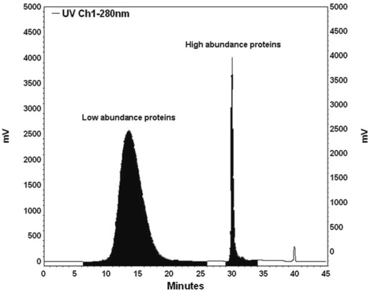
Immunodepletion chromatogram.

3.2. Protein Tagging

3.2.1. Protein Labeling with Acrylamide

1. Concentrate the control and disease immunodepleted plasma samples separately (only the flow-through low abundance protein fraction, see Fig. 2) in the Amicon YM-3 device until volume <100 μL. Do not mix or combine the control and disease samples.

2. Dilute each of the concentrated samples up to 1 mL with 8 M urea, 0.5 M TEAB (0.2% OG).

3. Measure protein concentration using Bradford method for disease and control samples, respectively (see Note 1).

4. Reduce protein disulfide bonds in each sample for 2 h at room temperature by adding 0.66 mg dithiothreitol (DTT) per milligram of protein.

5. Alkylate the samples with acrylamide isotopes immediately after the reduction by adding 7.1 mg/mg of total protein of light acrylamide to one of the samples (control or disease) and 7.4 mg/mg of total protein of heavy acrylamide to the other sample. The reaction is carried out for 1 h at room temperature. Keep the reaction in dark.

6. Mix or combine the control and disease samples, dilute it to 9 mL with Mobile-phase A of anion-exchange chromatography, and submit it immediately to 2D-HPLC protein separation.

3.2.2. Protein Labeling with iTRAQ (see Note 2)

1. Concentrate the control and disease immunodepleted plasma samples separately (only the flow-through low abundance protein fraction, see Fig. 2) in the Amicon YM-3 device until volume <100 μL. Do not mix or combine the control and disease samples.

2. Dilute each of the concentrated samples up to 4 mL with the iTRAQ Exchange Buffer: 6.6M Urea + 0.5 M TEAB + 0.2% OG (w/v). Concentrate the sample in the same Amicon YM-3 device until volume <100 μL to replace the immunodepletion Buffer A.

3. Repeat step 2 four times.

4. Measure protein concentration using Bradford method for disease and control samples, respectively.

5. Reduce protein disulfide bonds in each sample for 2 h at room temperature by adding 50 mM TCEP (20 μL/mg of protein).

6. Alkylate the samples immediately after the reduction by adding 200 mM iodoacetamide (10 μL/mg of protein). Keep the alkylation reaction in dark at room temperature for 1 h.

7. Add the iTRAQ solvent ETOH (from the iTRAQ kit) to each of the four iTRAQ reagent (corresponding to the reporter ion 114, 115, 116, and 117). Then, transfer them to each of the four under labeling samples. Each iTRAQ regent vial can be used for labeling 200 μg of protein.

8. Start the labeling reaction in dark at room temperature for 2 h.

9. Remove the organic solvent (ETOH) by Speed Vacuum Device and do not let the sample to dry totally.

10. Pool the four samples and dilute to 9 mL with anion-exchange Mobile Phase A.

11. Submit immediately to 2D-HPLC protein separation.

3.3. Protein Fractionation

3.3.1. The First Dimension Anion-Exchange Chromatography

Step-elution is listed in Table 2

Table 2. Anion-exchange chromatography step-elution, flow rate 0.8 mL/min.

Step-elution	Mobile phase B (%)
1	0.0
2	5.0
3	10.0
4	15.0
5	20.0
6	30.0
7	50.0
8	100.0

1. Equilibrate the anion-exchange column with Mobile-Phase A for 60 min at 0.8 mL/min.

2. Load the samples onto the 10 mL of sample-loop.

3. Start the run (see Fig. 2 for the online 2D-HPLC system diagram).

3.3.2. The Second Dimensional Reversed-Phase Chromatography

Gradient-elution: Flow rate: 2.4/min, UV = 280 nm

1. Equilibrate the two RP columns with 95% of Mobile-Phase A for 15 min before start the run.

2. Desalt the column with 95% Mobile-Phase A for 10 min before starting the gradient elution (see the gradient-elution in Table 3).

3. There is an 8-step-elution from anion-exchange column, and the RP gradient-elution will apply to each of the 8 step-elution of anion exchange chromatography. See Fig. 2 for the online 2D-HPLC system workflow diagram and a typical online 2D-HPLC chromatogram is shown in Fig. 4.

4. Collect the protein fractions from the RP column (3 fractions/min, 800 μL/fraction) and keep the protein fraction in −80°C.

5. Lyophilize the protein fractions using the Freeze Dry Systems (it usually takes 48 h to get the protein fraction dry completely).

Table 3. Reversed-phase chromatography gradient elution.

Time (min)	Buffer B (%)	Fraction collection
0.00	5.0
10.0	5.0	Start to collect the fraction, 3 fractions/ min, 800 μL/fraction
12.00	20
30.00	65
32.00	65
33.00	90
35.00	90
37.00	5.0
40.00	5.0	Stop to collect the fraction
46.00	Stop

Fig. 4.

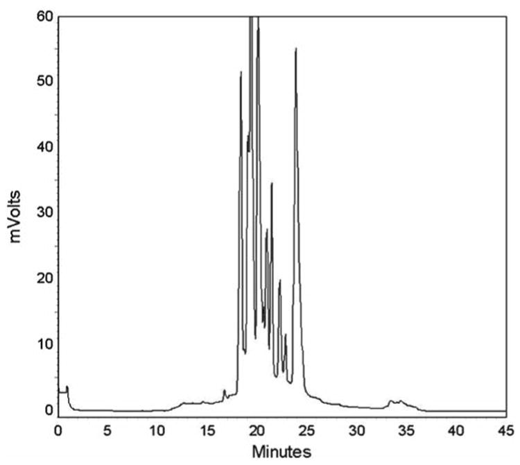
2D-HPLC Chromatogram (second dimension RP chromatography). Protein fractions collected between 10 and 40 min. A total of 84 fractions were collected.

3.4. Nano-LC ESI Mass Spectrometry Analysis

3.4.1. In-Solution Protein

1. Individual lyophilized protein fractions were suspended with 200 ng of trypsin in the digestion buffer. The digestion was performed at 37°C overnight.

2. The digestion was quenched by adding 5 μL of 1.0% formic acid solution.

3. Based on the RP chromatography pattern, individual fractions were combined to get 12-pooled fractions for nano-LC ESI mass spectrometry analysis. Table 4 lists the pooling sequence.

Table 4. Digested protein fraction pooling sequence for nano-LC ESI MS analysis.

Pool #	Fraction #
1	From fraction #04 to #22
2	From fraction #23 to #24
3	From fraction #25 to #26
4	From fraction #27 to #28
5	From fraction #29 to #30
6	From fraction #31 to #32
7	From fraction #33 to #34
8	From fraction #35 to #36
9	From fraction #37 to #38
10	From fraction #39 to #40
11	From fraction #41 to #42
12	From fraction #43 to #72

3.4.2. Nano Flow-Rate LC ESI Mass Spectrometry Analysis

Waters nano-Acquity UPLC is coupled with nano-ESI QTOF Premier, and Eksigent nano-LC-1D plus is coupled with nano-ESI LTQFT/or LTQ Orbitrap. Both nano-HPLC systems directly deliver nano flow rate without using splitter. The gradient elution program is listed in Table 5.

Table 5. Nano flow-rate reversed-phase HPLC gradient elution 300 nL/min.

Time (min)	Mobile phase B (%)
0.00	3.00
2.00	7.00
92.0	35.0
93.0	50.0
102.0	50.0
103.0	95.0
108.0	95.0
109.0	3.00
130.0	3.00

1. Load 10 μL of each pooled digested protein fraction into 20 μL of sample-loop.

2. After injection, sample is trapped onto the trap column and desalted with 3% of Mobile-phase B for 10 min at 4 μL/min

3. Start the nano-HPLC gradient elution and acquire spectra in a data-dependent mode in m/z range of 400 to 1,800. Select the five most abundant +2 or +3 ions of each MS spectrum for MS-MS analysis.

4. nano-ESI LTQFT mass spectrometer parameters are capillary voltage of 2.0 kV, capillary temperature of 200°C, resolution of 1,00,000, FT target value of 1,000,000, and ion trap target value of 10,000.

5. nano-ESI QTOF Premier mass spectrometer parameters are capillary voltage of 2.0 kV, nano-ESI source temperature of 150°C, resolution of 10,000, and MCP value of 2,300.

3.4.3. Data Analysis

The acquired QTOF data (for 4-plex iTRAQ labeling) is automatically processed with ProteinLynx Global Server 2.25

1. For databank search: Carbamidomethylation (C) was set as the fix modification, Oxidation (M) and iTRAQ (K and N terms) were set as the variable modification.

2. Peptide tolerance was set as 100 ppm, and fragment tolerance was set as 50 ppm. Missed cleavages were set as 3.

3. Figure 5 shows a representative nano flow-rate ESI MS (MS/ MS) analysis, including the TIC chromatogram, MS spectrum, MS/MS sequence spectrum, and iTRAQ reporter ions for quantitation.

Fig. 5.

4-plex iTRAQ analysis by nano-LC ESI QTOF Premier mass spectrometer. Four different plasma samples (after immunodepletion) were labeled with 4-plex iTRAQ reagent, respectively (with four reporter ion: 114.1, 115.1, 116.1, and 117.1). (a) The reconstructed total ion current (TIC) chromatogram corresponds to ∼2.5 μg of on-column loading (digested protein obtained from one pool of the 2D-HPLC fractionation, see Subheading 3.2.2). (b) The MS/MS sequence spectrum of precursor (m/z 618.29) and the quantifiable reporter ions from the low m/z range.

The acquired LTQFT data (for acrylamide labeling) is automatically processed by the Computational Proteomics Analysis System—CPAS (9, 10).

1. For databank search, D0-acrylamide alkylation was considered a fixed modification, and D3 isotope-labeled peptides were detected using a delta mass of 3.01884 Da (8). Acrylamide ratios are obtained by a script called “Q3,” which was developed in-house to obtain the relative quantification for each pair of peptides identified by MS/MS that contains cysteine residues.

2. Use the minimum criteria for peptide matching of Peptide Prophet score greater than 0.2 (16). Peptides that met these criteria are further grouped to protein sequences using the Protein Prophet algorithm at an error rate of 5% or less.

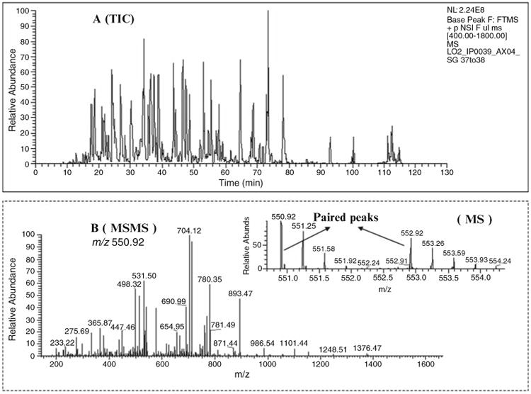
3. Figure 6 shows a representative nano flow-rate ESI MS (MS/ MS) analysis, including the TIC chromatogram, MS spectrum, MS/MS sequence spectrum, and acrylamide-labeled paired precursor ions for quantitation.

Fig. 6.

2-plex Acrylamide labeling analysis by nano-LC ESI LTQ-Orbitrap mass spectrometer. Two different plasma samples (after immunodepletion) were labeled with 2-plex Acrylamide (light and heavy) reagent, respectively. (a) The reconstructed total ion current (TIC) chromatogram corresponds to ∼2.5 μg of on-column loading (digested protein obtained from one pool of the 2D-HPLC fractionation, see Subheading 3.2.1). (b) The MS/MS sequence spectrum of precursor (m/z 550.92) and the quantifiable paired precursor ions from the MS scan.

4. Notes

1. As a result of the immunodepletion step, the total protein concentration is reduced by 90%, from ∼70 to 7 mg/mL.

2. Before the iTRAQ protein level labeling, the protein sample solution must be replaced with the exchange buffer with a pH 8.3 to avoid the labeling failure resulted from the free amine component in original sample solution and improper pH. Maintain 54% of organic solvent (ETOH) during the labeling reaction to keep 99% of labeling efficiency. After labeling reaction, remove ETOH before subject to 2D-HPLC separation because the higher percentage of organic solvent will result in sample loss during the loading step.

The feasibility of acrylamide labeling for protein identification and quantification has been demonstrated previously using MALDITOF for proteins separated by two-dimensional electrophoresis (13). No protein precipitation was observed, indicating that acrylamide-based alkylation is compatible with intact-protein-based approaches. A very high yield of cysteine alkylation is achieved (8). The interruption of reaction after 1 h is very important to avoid side reactions with free amines in the protein.

References

- 1.Fenn JB, Mann M, Meng CK, Wong SF, Whitehouse CM. Electrospray ionization for mass spectrometry of large biomolecules. Science. 1989;246:64–71. doi: 10.1126/science.2675315. [DOI] [PubMed] [Google Scholar]
- 2.Taflin DC, Ward TL, Davis EJ. Electrified droplet fission and the Rayleigh limit. Langmuir. 1989;5:376–384. [Google Scholar]
- 3.Dole M, Mack LL, Hines RL, Mobley RC, Ferguson LD, Alice MB. Molecular beams of macroions. J Chem Phys. 1968;49:2240–2249. [Google Scholar]
- 4.Iribarne JV, Thomson BA. On the evaporation of charged ions from small droplets. J Chem Phys. 1976;64:2287–2294. [Google Scholar]
- 5.Wilm M, Mann M. Analytical properties of the nanoelectrospray ion source. Anal Chem. 1996;68:1–8. doi: 10.1021/ac9509519. [DOI] [PubMed] [Google Scholar]
- 6.Wang H, Clouthier SG, Galchev V, Misek DE, Duffner U, Min CK, Zhao R, Tra J, Omenn GS, Ferrara JL, Hanash SM. Intact-protein based high-resolution three-dimensional quantitative analysis system for proteome profiling of biological fluids. Mol Cell Proteomics. 2005;4:618–25. doi: 10.1074/mcp.M400126-MCP200. [DOI] [PubMed] [Google Scholar]
- 7.Misek DE, Kuick R, Wang H, Galchev V, Bin Deng B, Zhao R, Tra J, Pisano MR, Amunugama R, Allen D, Walker AK, Strahler JR, Andrews P, Omenn GS, Hanash SM. A wide range of protein isoforms in serum and plasma uncovered by a quantitative intact protein analysis system. Proteomics. 2005;5:3343–3352. doi: 10.1002/pmic.200500103. [DOI] [PubMed] [Google Scholar]
- 8.Faca V, Coram M, Phanstiel D, Glukhova V, Zhang Q, Fitzgibbon M, McIntosh M, Hanash S. Quantitative analysis of acrylamide labeled serum proteins by LC-MS/ MS. J Proteome Res. 2006;5:2009–2018. doi: 10.1021/pr060102+. [DOI] [PubMed] [Google Scholar]
- 9.Rauch A, Bellew M, Eng J, Fitzgibbon M, Holzman T, Hussey P, Igra M, Maclean B, Lin CW, Detter A, Fang R, Faca V, Gafken P, Zhang H, Whitaker J, States D, Hanash S, Paulovich A, McIntosh MW. Computational Proteomics Analysis System (CPAS): an extensible, open-source analytic system for evaluating and publishing proteomic data and high throughput biological experiments. J Proteome Res. 2006;5:112–121. doi: 10.1021/pr0503533. [DOI] [PubMed] [Google Scholar]
- 10.Maclean B, Eng JK, Beavis RC, McIntosh M. General framework for developing and evaluating database scoring algorithms using the TANDEM search engine. Bioinformatics. 2006 doi: 10.1093/bioinformatics/btl379. [DOI] [PubMed] [Google Scholar]
- 11.Keller A, Nesvizhskii AI, Kolker E, Aebersold R. Empirical statistical model to estimate the accuracy of peptide identifications made by MS/MS and database search. Anal Chem. 2002;74:5383–5392. doi: 10.1021/ac025747h. [DOI] [PubMed] [Google Scholar]
- 12.Nesvizhskii AI, Keller A, Kolker E, Aebersold R. A statistical model for identifying proteins by tandem mass spectrometry. Anal Chem. 2003;75:4646–4658. doi: 10.1021/ac0341261. [DOI] [PubMed] [Google Scholar]
- 13.Sechi S, Chait BT. Modification of cysteine residues by alkylation. A tool in peptide mapping and protein identification. Anal Chem. 1998;70:5150–5158. doi: 10.1021/ac9806005. [DOI] [PubMed] [Google Scholar]