

Abstract
In this paper, we develop methods for longitudinal quantile regression when there is monotone missingness. In particular, we propose pattern mixture models with a constraint that provides a straightforward interpretation of the marginal quantile regression parameters. Our approach allows sensitivity analysis which is an essential component in inference for incomplete data. To facilitate computation of the likelihood, we propose a novel way to obtain analytic forms for the required integrals. We conduct simulations to examine the robustness of our approach to modeling assumptions and compare its performance to competing approaches. The model is applied to data from a recent clinical trial on weight management.
Keywords: Marginalized models, Non-ignorable missingness, Pattern mixture models
1. Introduction
Quantile regression is used to study the relationship between a response and covariates when one (or several) quantiles are of interest as opposed to mean regression. The dependence between upper or lower quantiles of the response variable and the covariates often vary differentially relative to that of the mean. How quantiles depend on covariates is of interest in econometrics, educational studies, biomedical studies, and environment studies (Yu and Moyeed, 2001; Buchinsky, 1994, 1998; He and others, 1998; Koenker and Machado, 1999; Wei and others, 2006; Yu and others, 2003). A comprehensive review of applications of quantile regression was presented in Koenker (2005).
Quantile regression is more robust to outliers than mean regression and provides information about how covariates affect quantiles, which offers a more complete description of the conditional distribution of the response. Different effects of covariates can be assumed for different quantiles.
The traditional frequentist approach was proposed by Koenker and Bassett (1978) for a single quantile with estimators derived by minimizing a loss function. The popularity of this approach is due to its computational efficiency, well-developed asymptotic properties, and straightforward extensions to simultaneous quantile regression and random effect models. However, the approach does not naturally extend to missing data. Extensions of minimizing a loss function include the use of regularization. Koenker (2004) adopted  regularization methods to shrink a large number of individual effects to a common value for quantile regression models for longitudinal data. Li and Zhu (2008) considered
  -norm (LASSO) regularized quantile regression. Wu and Liu (2009) used a smoothly clipped absolute deviation model for variable selection in penalized quantile regression. In terms of Bayesian inference, both parametric and semiparametric Bayesian approaches have been proposed in the literature (Yu and Moyeed, 2001; Walker and Mallick, 1999; Hanson and Johnson, 2002; Reich and others, 2010).
All the above methods focus on complete data. There are only a few articles about quantile regression with missingness. Wei and others (2012) proposed a multiple imputation method for quantile regression model when there are some covariates missing at random (MAR). They impute the missing covariates by specifying its conditional density given observed covariance and outcomes; this density come from the estimated conditional quantile regression and specification of conditional density of missing covariates given observed ones. However, they focus more on the missing covariates than missing outcomes. Bottai and Zhen (2013) introduced an imputation method using estimated conditional quantiles of missing outcomes given observed data. Their approach does not make distributional assumptions. They assumed the missing data mechanism (MDM) is MAR. However, because their imputation method is not derived from a joint distribution, the joint distribution under such conditionals may not exist. In addition, their approach does not allow for missing not at random (MNAR). Farcomeni and Viviani (2015) assumed an asymmetric Laplace distribution (LP) for the error distribution of the longitudinal model and adopted Monte Carlo Expectation Maximization method for a longitudinal quantile regression in the presence of informative dropout through longitudinal-survival joint model. However, the parametric assumption of error distribution may not be realistic.
Yuan and Yin (2010) introduced a Bayesian quantile regression approach for longitudinal data with non-ignorable missing data. They used shared latent subject-specific random effects to explain the within-subject correlation and to associate the response process with missing data process, and applied multivariate normal priors on the random terms to match the standard quantile regression check function with penalties. However, the quantile regression coefficients are conditional on the random effects, which is not of interest if we are interested in interpreting regression coefficients unconditionally. In addition, they are conditional on random effects, which tie together the responses and missingness process, so they have a slightly different interpretation than typical random effects in longitudinal methods. Another important point is that all the models mentioned above do not allow for sensitivity analysis, which is a key component in inference for incomplete data (National Research Council, 2010).
Pattern mixture models were originally proposed to model missing data in Rubin (1977). Later mixture models were extended to handle MNAR in longitudinal data. For discrete dropout times, Little (1993, 1994) proposed a general method by introducing a finite mixture of multivariate distributions for longitudinal data. When there are many possible dropout time, Roy (2003) proposed to group them by latent classes.
Roy and Daniels (2008) extended Roy (2003) to generalized linear models and proposed a pattern mixture model for data with non-ignorable dropout, borrowing ideas from Heagerty (1999). But their approach only estimates the marginal covariate effects on the mean. We will use related ideas for quantile regression models which allow for non-ignorable missingness and sensitivity analysis.
The structure of this article is as follows. First, we introduce a quantile regression method to address monotone non-ignorable missingness in Section 2, including sensitivity analysis and computational details. We use simulation studies to evaluate the performance of the model in Section 3. We apply our approach to data from a recent clinical trial in Section 4. Finally, discussion and conclusions are given in Section 5.
2. Model
In this section, we first introduce some notation, then describe our proposed quantile regression model in Section 2.1. We provide details on MAR and MNAR and computation in Sections 2.2 and 2.3, respectively.
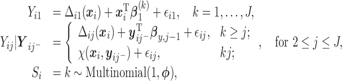
Under monotone dropout, denote  to be the number of observed
  for subject
  , and
, and  to be the full-data response vector for subject
  , where
  correspond to the maximum follow-up time. We assume that
  is always observed. We are interested in the
  th marginal quantile regression coefficients
  ,
,
 |
(2.1) |
where  is a
is a  vector of covariates for subject
  .
.
Let  and
and  be the conditional densities of response
  given covariates
  and
and  and
and  , respectively. And
  .
.
2.1. Mixture model specification
We adopt a pattern mixture model to jointly model the response and missingness (Little, 1994; Daniels and Hogan, 2008). Mixture models factor the joint distribution of response and missingness as
 |
Thus, the full-data response follows the distribution given by
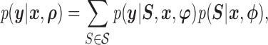 |
where  is the sample space for the number of observed responses,
  (i.e. the pattern) and the full parameter vector
  is partitioned as
  .
.
Furthermore, the conditional distribution of response within patterns can be decomposed as
 |
(2.2) |
where  is the missing data,
  is the observed data,
  ,
,  indexes the parameters in the extrapolation distribution, the first term on the right-hand side and
  indexes parameters in the distribution of observed responses, the second term on the right-hand side. The entire vector of parameters indexing the observed data,
  will be denoted as
  . We re-state the definition of sensitivity parameters from Hogan and others (2014); note that a different, but equivalent definition can be found in Daniels and Hogan (2008). Define
 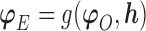 . The parameter
  is a sensitivity parameter if (1) the parameter
  is non-identifiable in the sense that
  ; (2) the parameter
  is identifiable; (3) the known function
  is non-constant in
  . The first condition states that the observed data contribute no information about the sensitivity parameter. The second and third conditions imply that the full-data model is identified for a fixed
  .
.
We assume a sequential finite ( ) mixture of normals within each pattern. A random variable
  follows a finite (
 ) mixture of normal distribution (MN), when
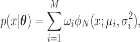 |
where 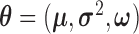 ,
,  , and
, and  denotes the PDF evaluated at
  of a normal distribution with mean
  and variance
  .
.
We specify the distributions conditional on  as:
as:
 |
(2.3) |
where
 |
(2.4) |
with the marginal quantile regression constraints (2.1). The parameter  is the shift of the coefficients for distribution of
  ,
,  is the response history for subject
  up to time point
  ,
,  are autoregressive coefficients,
  is the conditional standard deviation of response component
  , and
, and  is the multinomial probability vector for the number of observed responses.
  are subject/time specific intercepts determined by the parameters in (2.1) and (2.3); more details are given in what follows.
  is the mean of the unobserved data distribution and allows sensitivity analysis by varying assumptions on
  ; for computational reasons, we assume that
  is linear in
  . For example, here we specify
 |
(2.5) |
where  is a set of sensitivity parameters and
  is a function of
  . Comparing (2.3) and (2.5), the mean of the unidentified distribution,
  for
for  is characterized by an intercept shift from identified observed data distribution,
  for
for  . More details about sensitivity parameters are given in Section 2.2.
For (standard) identifiability of the distribution of the observed data, we use the following restrictions (without loss of generality),  . Also in order to not confound the marginal quantile regression parameters, we put the following constraint on the parameters
  in the mixture of normals distribution,
  .
.
In (2.3) and (2.5),  are also functions of
  and are determined by the marginal quantile regressions,
 |
(2.6) |
and
 |
(2.7) |
Details on computing the  will be given in Section 2.3. The expressions in (2.6) and (2.7) show how the marginal quantiles are related to the models conditional on only the number of observed responses at the first time point, (2.6) and conditional on the number of observed responses and the previous history of responses at subsequent times, (2.7). These equalities determine the intercept parameters,
  in the conditional models in (2.3).
The idea in the above specification is to model the marginal quantile regressions directly and then to embed them in the likelihood through restrictions in the mixture model. The finite mixture of normals distribution makes the model flexible and accommodates heavy tails, skewness, and multi-modality. The mixture model in (2.3) allows the marginal quantile regression coefficients to differ by quantiles; otherwise, the quantile lines would be parallel to each other. Moreover, the mixture model also allows sensitivity analysis for the missing data. This is an essential component of the analysis of missing data (as discussed in Section 1) and is not possible in previous approaches.
2.2. MDM and sensitivity analysis
Mixture models as specified in Section 2.1 are not identified by the observed data (as stated in the previous subsection). Specific forms of missingness induce constraints to identify the distributions for incomplete patterns, in particular, the extrapolation distribution in (2.2). In this section, we explore ways to embed the missingness mechanism and sensitivity parameters in mixture models for our setting.
In the mixture model in (2.3), MAR holds (Molenberghs and others, 1998; Wang and Daniels, 2011) if and only if, for each  and
and  :
:
 |
When  and
and  ,
,  is not observed, thus
  cannot be identified from the observed data and is a set of sensitivity parameters as defined earlier.
When  , MAR holds. If
  is fixed at
  , the missingness mechanism is MNAR. We can vary
  around
  to examine the impact of different MNAR mechanisms.
In general, each pattern  has its own set of sensitivity parameters
  . However, to keep the number of sensitivity parameters at a manageable level (Daniels and Hogan, 2008) and without loss of generality in what follows, we assume
  does not depend on pattern.
2.3. Computation
In Section 2.3.1, we provide details on calculating  in (2.3) for
  . Then we show how to obtain maximum likelihood estimates in Section 2.3.2.
2.3.1. Calculation of 
From (2.6) and (2.7),  is a function of subject-specific covariates
  , thus
  needs to be calculated for each subject. We now illustrate how to calculate
  given all the other parameters
  .
.
-
 : Given the result in Lemma 0.1 in supplementary material available at Biostatistics online, to solve (2.7), we propose a recursive approach. Expand (2.7) with (2.3) and (2.4):
For the first multiple integral in (2.7), apply Lemma 0.1 once to obtain: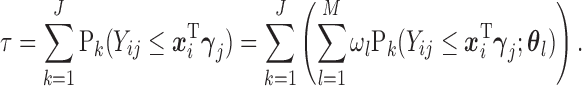
where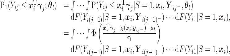
and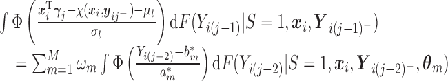
when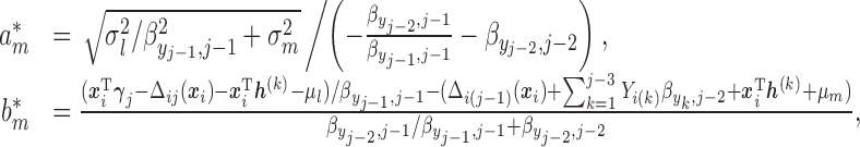
 takes the linear form given in (2.5) with
  . Similar results hold as long as
  is linear in
  .
.Then, by recursively applying Lemma 0.1
 times, each multiple integral in (2.7) can be simplified to single normal CDF. Thus, we can easily solve for
  using standard numerical root-finding method as for
  .
.


2.3.2. Maximum likelihood estimation
The observed data likelihood for an individual  with follow-up time
  is
is
 |
(2.8) |
where  .
.
We use derivative-free optimization algorithms by quadratic approximation to compute the maximum likelihood estimates (Bates and others, 2012). Denote  . Then maximizing the likelihood is equivalent to minimizing the target function
  .
.
During each step of the algorithm,  has to be calculated for each subject and at each time, as well as partial derivatives for each parameter.
As an example of the speed of the algorithm, for 100 bivariate outcomes and 5 covariates, it takes about 1.9 s to obtain convergence using R version 2.15.3 (2013-03-01) (R Core Team, 2013) and platform: x86_64-apple-darwin9.8.0/x86_64 (64-bit). Main parts of the algorithm are coded in Fortran such as calculation of numerical derivatives and log-likelihood to quicken computations. We have incorporated those functions implementing the algorithm into the new R (R Core Team, 2013) package “qrmissing”.
We use the bootstrap (Efron and Tibshirani, 1993) to construct confidence interval and make inferences. We re-sample subjects and use bootstrap percentile intervals to form confidence intervals. We use the bayesian information criterion (BIC) to select the number of components in the mixture of normals in (2.3).
3. Simulation study
In this section, we compare the performance of our proposed model with the approach in (Koenker, 2004) (denoted as RQ) in quantreg R package (Koenker, 2012), Bottai's algorithm (Bottai and Zhen, 2013) (denoted as BZ) and the approach introduced in (Lipsitz and others, 1997) (denoted as LF). The rq function minimizes the loss (check) function  in terms of
  , where the loss function
  and does not make any distributional assumptions, but does not accommodate MAR or MNAR missingness. The method employs
  regularization to shrink the individual effects toward a common value, to mollify the inflation effect in longitudinal quantile regression. Bottai and Zhen (2013) impute missing outcomes using the estimated conditional quantiles of missing outcomes given observed data. Their approach does not make distributional assumptions similar to RQ and assumes MAR missingness, but also does not allow MNAR missingness. Lipsitz and others (1997) introduced “weighted” estimating equations in quantile regression models for longitudinal data with drop-outs. After the appropriate re-weighting, the estimating equations can be solved by traditional quantile regression method in quantreg R package. This approach also does not make any assumptions about the distribution of the responses and assumes that the missingness is MAR.
We considered 3 scenarios corresponding to both MAR and MNAR assumptions for a bivariate response.  were always observed, while some of
  were missing. In the first scenario,
  were MAR and we used the MAR assumption in our algorithm. In the next 2 scenarios,
  were MNAR. However, in the second scenario, we misspecified the MDM for our algorithm and still assumed MAR, while in the third scenario, we used the correct MNAR MDM. For each scenario, we considered 4 error distributions: normal, Student
  distribution with 3 degrees of freedom, Laplace distribution, and a mixture of normal distribution. For each error model, we simulated 100 data sets. For each dataset, there are 200 bivariate observations
  for
for  . A single covariate
  was sampled from Uniform(0,2). The 4 models for the full-data response
  were:
were:
 |
where  ,
,  ,
,  , and
, and  distributions within each scenario, where
  and
and  . For all cases,
  . When
  ,
,  is not observed, so
  is not identifiable from observed data. In the first scenario,
  is MAR, thus
  . In the last 2 scenarios,
  are MNAR. We assume
  . Therefore, there is a shift of 2 in the intercept between
  and
and  .
.
Under an MAR assumption, the sensitivity parameter  is fixed at
  as discussed in Section 2.2. For rq function from quantreg R package, because only
  is observed, the quantile regression for
  can only be fit from the information of
  vs
vs  .
.
In scenario 2 under MNAR, we misspecified the MDM using the wrong sensitivity parameter, setting  . In scenario 3, we correctly assumed there was a non-zero intercept shift between distribution of
  and
and  ,
,  , fixing
  at its true value.
For each dataset, we fit quantile regression for quantiles  , 0.3, 0.5, 0.7, 0.9. Parameter estimates were evaluated by mean squared error (MSE),
 |
where  is the true value for quantile regression coefficient,
  is the maximum likelihood estimates in
  th simulated dataset (
 for
for  ,
,  for
for  ).
).
The true values for quantile regression coefficients are obtained through the following procedures:
Generate
 evenly spaced in the range of
  .
.For each
 , compute the
  th conditional quantile of
  , denoted as
  .
.Regress
 on
on  to compute the regression coefficients (the
  th quantile regression coefficients).
Tables 1–3 present the MSE for coefficients estimates of quantile 0.1, 0.3, 0.5, 0.7, 0.9 under each scenario. M1 stands for the proposed model with  , and M2 stands for the model with
  chosen by the BIC.
Table 2.
Scenario 2: MSE for coefficients estimates of quantiles  under MNAR scenario
 |
 |
LP |
Mix |
|||||||||||||||||
|---|---|---|---|---|---|---|---|---|---|---|---|---|---|---|---|---|---|---|---|---|
| M1 | M2 | RQ | BZ | LF | M1 | M2 | RQ | BZ | LF | M1 | M2 | RQ | BZ | LF | M1 | M2 | RQ | BZ | LF | |
| 10% | ||||||||||||||||||||

|
0.08 | 0.07 | 0.10 | 0.10 | 0.15 | 0.31 | 0.13 | 0.22 | 0.21 | 218.71 | 2.04 | 1.20 | 1.91 | 1.94 | 79.32 | 0.44 | 0.21 | 0.24 | 0.24 | 2.17 |

|
0.04 | 0.04 | 0.07 | 0.07 | 0.20 | 0.09 | 0.06 | 0.13 | 0.13 | 223.69 | 0.31 | 0.16 | 0.62 | 0.62 | 394.69 | 0.22 | 0.13 | 0.18 | 0.18 | 4.87 |

|
0.11 | 0.11 | 0.37 | 0.10 | 0.39 | 0.35 | 0.12 | 0.76 | 0.21 | 257.46 | 3.88 | 3.70 | 7.32 | 1.94 | 146.54 | 0.36 | 0.23 | 1.11 | 0.24 | 3.89 |

|
0.06 | 0.06 | 0.12 | 0.07 | 0.12 | 0.13 | 0.08 | 0.27 | 0.13 | 75.69 | 0.33 | 0.24 | 1.07 | 0.62 | 36.55 | 0.26 | 0.19 | 0.26 | 0.18 | 1.04 |
| 30% | ||||||||||||||||||||

|
0.12 | 0.10 | 0.12 | 0.12 | 0.15 | 0.17 | 0.10 | 0.16 | 0.16 | 202.42 | 0.21 | 0.20 | 0.41 | 0.40 | 206.66 | 0.49 | 0.20 | 0.73 | 0.73 | 4.86 |

|
0.05 | 0.04 | 0.09 | 0.09 | 0.12 | 0.09 | 0.06 | 0.12 | 0.11 | 224.45 | 0.25 | 0.16 | 0.36 | 0.36 | 246.05 | 0.18 | 0.05 | 0.75 | 0.75 | 2.90 |

|
0.08 | 0.08 | 0.80 | 0.12 | 0.85 | 0.18 | 0.10 | 0.77 | 0.16 | 161.38 | 0.91 | 0.53 | 2.07 | 0.40 | 108.47 | 0.32 | 0.32 | 2.74 | 0.73 | 8.92 |

|
0.07 | 0.07 | 0.07 | 0.09 | 0.09 | 0.15 | 0.09 | 0.08 | 0.11 | 76.01 | 0.34 | 0.25 | 0.35 | 0.36 | 38.34 | 0.19 | 0.10 | 0.55 | 0.75 | 1.17 |
| 50% | ||||||||||||||||||||

|
0.25 | 0.24 | 1.33 | 1.34 | 1.57 | 0.09 | 0.18 | 1.08 | 1.13 | 236.03 | 0.22 | 0.19 | 0.97 | 0.95 | 216.33 | 0.12 | 0.03 | 0.25 | 0.27 | 2.28 |

|
0.97 | 0.99 | 2.68 | 2.86 | 2.96 | 0.49 | 0.59 | 1.83 | 1.89 | 219.73 | 0.24 | 0.28 | 1.17 | 1.13 | 134.10 | 0.19 | 0.10 | 0.49 | 0.52 | 1.63 |

|
1.26 | 1.14 | 4.14 | 1.34 | 4.15 | 1.32 | 1.19 | 4.19 | 1.13 | 94.29 | 1.49 | 1.28 | 4.43 | 0.95 | 199.87 | 1.06 | 0.93 | 4.63 | 0.27 | 13.94 |

|
0.08 | 0.08 | 0.30 | 2.86 | 0.30 | 0.16 | 0.07 | 0.33 | 1.89 | 73.77 | 0.22 | 0.18 | 0.43 | 1.13 | 120.89 | 0.20 | 0.09 | 0.68 | 0.52 | 2.16 |
| 70% | ||||||||||||||||||||

|
0.10 | 0.07 | 0.27 | 0.13 | 0.13 | 0.18 | 0.06 | 0.15 | 0.07 | 340.51 | 0.32 | 0.25 | 0.36 | 0.37 | 263.39 | 0.47 | 0.17 | 0.62 | 0.69 | 4.80 |

|
0.06 | 0.04 | 0.15 | 0.09 | 0.10 | 0.12 | 0.04 | 0.17 | 0.10 | 224.24 | 0.30 | 0.21 | 0.43 | 0.37 | 191.70 | 0.17 | 0.03 | 0.70 | 0.59 | 2.52 |

|
4.74 | 4.60 | 11.00 | 0.13 | 10.29 | 4.11 | 4.32 | 11.35 | 0.07 | 61.02 | 2.45 | 2.50 | 9.00 | 0.37 | 166.67 | 1.89 | 1.24 | 6.90 | 0.69 | 16.16 |

|
0.15 | 0.15 | 1.09 | 0.09 | 1.12 | 0.30 | 0.15 | 1.07 | 0.10 | 76.59 | 0.38 | 0.27 | 1.48 | 0.37 | 181.60 | 0.22 | 0.10 | 1.13 | 0.59 | 3.09 |
| 90% | ||||||||||||||||||||

|
0.07 | 0.07 | 0.11 | 0.09 | 0.10 | 0.25 | 0.07 | 0.15 | 0.14 | 373.57 | 2.44 | 1.35 | 1.72 | 2.13 | 185.91 | 0.39 | 0.18 | 0.24 | 0.21 | 1.03 |

|
0.05 | 0.05 | 0.07 | 0.06 | 0.15 | 0.13 | 0.05 | 0.13 | 0.14 | 209.69 | 0.37 | 0.24 | 0.57 | 0.53 | 207.99 | 0.16 | 0.09 | 0.22 | 0.19 | 0.98 |

|
6.33 | 6.05 | 16.72 | 0.09 | 13.30 | 4.79 | 4.87 | 15.47 | 0.14 | 37.97 | 1.06 | 0.68 | 5.85 | 2.13 | 58.23 | 2.57 | 2.12 | 6.67 | 0.21 | 20.14 |

|
0.14 | 0.12 | 1.24 | 0.06 | 1.59 | 0.32 | 0.13 | 1.46 | 0.14 | 88.49 | 0.40 | 0.26 | 3.37 | 0.53 | 257.12 | 0.26 | 0.14 | 2.62 | 0.19 | 14.97 |
In this scenario, we adopted MAR assumption for our approach and thus misspecified the MDM.  are quantile regression coefficients for
  and
and  are coefficients for
  . M
. M stands for our proposed method with
  M
M stands for proposed model with
  chosen by BIC, RQ stands for the method implemented in Koenker (2004), BZ stands for Bottai's approach, and LF stands for the approach in Lipsitz and others (1997). The titles for sub-columns indicate models with 4 errors distributed from: Normal (
 ),
),  distribution with degrees of freedom
  LP, and mixture of 2 normals (Mix).
Table 1.
Scenario 1: MSE for coefficients estimates of quantiles  under MAR assumptions
| N |
 |
LP |
Mix |
|||||||||||||||||
|---|---|---|---|---|---|---|---|---|---|---|---|---|---|---|---|---|---|---|---|---|
| M1 | M2 | RQ | BZ | LF | M1 | M2 | RQ | BZ | LF | M1 | M2 | RQ | BZ | LF | M1 | M2 | RQ | BZ | LF | |
| 10% | ||||||||||||||||||||

|
0.08 | 0.07 | 0.10 | 0.10 | 0.15 | 0.31 | 0.13 | 0.22 | 0.21 | 218.71 | 2.04 | 1.20 | 1.91 | 1.94 | 79.32 | 0.44 | 0.21 | 0.24 | 0.24 | 2.17 |

|
0.04 | 0.04 | 0.07 | 0.07 | 0.20 | 0.09 | 0.06 | 0.13 | 0.13 | 223.69 | 0.31 | 0.16 | 0.62 | 0.62 | 394.69 | 0.22 | 0.13 | 0.18 | 0.18 | 4.87 |

|
0.11 | 0.11 | 0.36 | 0.10 | 0.38 | 0.31 | 0.10 | 0.66 | 0.21 | 256.64 | 3.55 | 3.37 | 6.88 | 1.94 | 145.25 | 0.37 | 0.23 | 1.02 | 0.24 | 3.72 |

|
0.06 | 0.06 | 0.12 | 0.07 | 0.12 | 0.13 | 0.07 | 0.28 | 0.13 | 75.55 | 0.31 | 0.22 | 1.08 | 0.62 | 36.38 | 0.24 | 0.18 | 0.26 | 0.18 | 1.01 |
| 30% | ||||||||||||||||||||

|
0.12 | 0.10 | 0.12 | 0.12 | 0.15 | 0.17 | 0.10 | 0.16 | 0.16 | 202.42 | 0.21 | 0.20 | 0.41 | 0.40 | 206.66 | 0.49 | 0.20 | 0.73 | 0.73 | 4.86 |

|
0.05 | 0.04 | 0.09 | 0.09 | 0.12 | 0.09 | 0.06 | 0.12 | 0.11 | 224.45 | 0.25 | 0.16 | 0.36 | 0.36 | 246.05 | 0.18 | 0.05 | 0.75 | 0.75 | 2.90 |

|
0.10 | 0.10 | 0.64 | 0.12 | 0.69 | 0.13 | 0.08 | 0.56 | 0.16 | 160.22 | 0.75 | 0.42 | 1.78 | 0.40 | 106.89 | 0.32 | 0.12 | 1.56 | 0.73 | 6.53 |

|
0.06 | 0.06 | 0.08 | 0.09 | 0.09 | 0.13 | 0.07 | 0.09 | 0.11 | 75.74 | 0.31 | 0.23 | 0.35 | 0.36 | 37.97 | 0.18 | 0.08 | 0.65 | 0.75 | 1.03 |
| 50% | ||||||||||||||||||||

|
0.25 | 0.24 | 1.33 | 1.34 | 1.57 | 0.09 | 0.18 | 1.08 | 1.13 | 236.03 | 0.22 | 0.19 | 0.97 | 0.95 | 216.33 | 0.12 | 0.03 | 0.25 | 0.27 | 2.28 |

|
0.97 | 0.99 | 2.68 | 2.86 | 2.96 | 0.49 | 0.59 | 1.83 | 1.89 | 219.73 | 0.24 | 0.28 | 1.17 | 1.13 | 134.10 | 0.19 | 0.10 | 0.49 | 0.52 | 1.63 |

|
0.17 | 0.13 | 1.11 | 1.34 | 1.12 | 0.19 | 0.11 | 1.14 | 1.13 | 86.01 | 0.37 | 0.27 | 1.33 | 0.95 | 184.00 | 0.26 | 0.12 | 1.86 | 0.27 | 8.54 |

|
0.08 | 0.08 | 0.30 | 2.86 | 0.30 | 0.16 | 0.07 | 0.33 | 1.89 | 73.77 | 0.22 | 0.18 | 0.43 | 1.13 | 120.89 | 0.18 | 0.07 | 0.80 | 0.52 | 1.97 |
| 70% | ||||||||||||||||||||

|
0.10 | 0.07 | 0.27 | 0.13 | 0.13 | 0.18 | 0.06 | 0.15 | 0.07 | 340.51 | 0.32 | 0.25 | 0.36 | 0.37 | 263.39 | 0.47 | 0.17 | 0.62 | 0.69 | 4.80 |

|
0.06 | 0.04 | 0.15 | 0.09 | 0.10 | 0.12 | 0.04 | 0.17 | 0.10 | 224.24 | 0.30 | 0.21 | 0.43 | 0.37 | 191.70 | 0.17 | 0.03 | 0.70 | 0.59 | 2.52 |

|
0.20 | 0.17 | 2.07 | 0.13 | 1.83 | 0.29 | 0.21 | 2.34 | 0.07 | 45.02 | 0.66 | 0.49 | 1.50 | 0.37 | 136.81 | 0.32 | 0.12 | 2.88 | 0.69 | 9.54 |

|
0.13 | 0.13 | 0.97 | 0.09 | 1.00 | 0.28 | 0.13 | 0.95 | 0.10 | 76.85 | 0.35 | 0.25 | 1.36 | 0.37 | 182.29 | 0.22 | 0.10 | 1.09 | 0.59 | 3.16 |
| 90% | ||||||||||||||||||||

|
0.07 | 0.07 | 0.11 | 0.09 | 0.10 | 0.25 | 0.07 | 0.15 | 0.14 | 373.57 | 2.44 | 1.35 | 1.72 | 2.13 | 185.91 | 0.39 | 0.18 | 0.24 | 0.21 | 1.03 |

|
0.05 | 0.05 | 0.07 | 0.06 | 0.15 | 0.13 | 0.05 | 0.13 | 0.14 | 209.69 | 0.37 | 0.24 | 0.57 | 0.53 | 207.99 | 0.16 | 0.09 | 0.22 | 0.19 | 0.98 |

|
0.48 | 0.43 | 4.52 | 0.09 | 2.93 | 0.46 | 0.34 | 4.28 | 0.14 | 23.11 | 3.10 | 2.81 | 1.93 | 2.13 | 38.24 | 0.48 | 0.24 | 2.25 | 0.21 | 11.80 |

|
0.13 | 0.12 | 1.23 | 0.06 | 1.58 | 0.31 | 0.12 | 1.39 | 0.14 | 88.73 | 0.39 | 0.24 | 3.25 | 0.53 | 257.90 | 0.27 | 0.14 | 2.81 | 0.19 | 14.64 |
 are quantile regression coefficients for
  and
and  are coefficients for
  . M
. M stands for our proposed method with
  M
M stands for proposed model with
  chosen by BIC, RQ stands for the method implemented in Koenker (2004), BZ stands for Bottai's approach, and LF stands for the approach in Lipsitz and others (1997). The titles for sub-columns indicate models with 4 errors distributed from: Normal (
 ),
),  distribution with degrees of freedom
  Laplace distribution (LP), and mixture of 2 normals (Mix).
Table 3.
Scenario 3: MSE for coefficients estimates of quantiles  under MNAR scenario
 |
 |
LP |
Mix |
|||||||||||||||||
|---|---|---|---|---|---|---|---|---|---|---|---|---|---|---|---|---|---|---|---|---|
| M1 | M2 | RQ | BZ | LF | M1 | M2 | RQ | BZ | LF | M1 | M2 | RQ | BZ | LF | M1 | M2 | RQ | BZ | LF | |
| 10% | ||||||||||||||||||||

|
0.10 | 0.09 | 0.10 | 0.10 | 0.15 | 0.27 | 0.14 | 0.22 | 0.21 | 218.71 | 2.23 | 1.25 | 2.04 | 2.08 | 67.13 | 0.52 | 0.17 | 0.24 | 0.24 | 2.17 |

|
0.06 | 0.06 | 0.07 | 0.07 | 0.20 | 0.12 | 0.07 | 0.13 | 0.13 | 223.69 | 0.40 | 0.22 | 0.61 | 0.62 | 348.72 | 0.20 | 0.10 | 0.18 | 0.18 | 4.87 |

|
0.17 | 0.14 | 0.37 | 0.10 | 0.39 | 0.31 | 0.14 | 0.76 | 0.21 | 257.46 | 2.81 | 2.32 | 6.73 | 2.08 | 98.71 | 0.60 | 0.25 | 1.11 | 0.24 | 3.89 |

|
0.09 | 0.06 | 0.12 | 0.07 | 0.12 | 0.16 | 0.09 | 0.27 | 0.13 | 75.69 | 0.45 | 0.26 | 1.04 | 0.62 | 26.61 | 0.32 | 0.13 | 0.26 | 0.18 | 1.04 |
| 30% | ||||||||||||||||||||

|
0.22 | 0.09 | 0.12 | 0.12 | 0.15 | 0.20 | 0.11 | 0.16 | 0.16 | 202.42 | 0.27 | 0.25 | 0.38 | 0.37 | 204.99 | 0.49 | 0.16 | 0.73 | 0.73 | 4.86 |

|
0.17 | 0.04 | 0.09 | 0.09 | 0.12 | 0.12 | 0.06 | 0.12 | 0.11 | 224.45 | 0.25 | 0.18 | 0.31 | 0.31 | 251.12 | 0.18 | 0.05 | 0.75 | 0.75 | 2.90 |

|
0.25 | 0.17 | 0.80 | 0.12 | 0.85 | 0.23 | 0.13 | 0.77 | 0.16 | 161.38 | 0.45 | 0.27 | 2.10 | 0.37 | 80.42 | 0.50 | 0.37 | 2.74 | 0.73 | 8.92 |

|
0.11 | 0.06 | 0.07 | 0.09 | 0.09 | 0.17 | 0.07 | 0.08 | 0.11 | 76.01 | 0.36 | 0.20 | 0.36 | 0.31 | 28.86 | 0.24 | 0.10 | 0.55 | 0.75 | 1.17 |
| 50% | ||||||||||||||||||||

|
0.32 | 0.29 | 1.33 | 1.34 | 1.57 | 0.10 | 0.19 | 1.08 | 1.13 | 236.03 | 0.22 | 0.22 | 0.93 | 0.92 | 218.40 | 0.12 | 0.03 | 0.25 | 0.27 | 2.28 |

|
1.03 | 1.03 | 2.68 | 2.86 | 2.96 | 0.54 | 0.56 | 1.83 | 1.89 | 219.73 | 0.22 | 0.24 | 1.08 | 1.06 | 141.01 | 0.21 | 0.11 | 0.49 | 0.52 | 1.63 |

|
0.29 | 0.22 | 4.14 | 1.34 | 4.15 | 0.21 | 0.18 | 4.19 | 1.13 | 94.29 | 0.40 | 0.30 | 4.43 | 0.92 | 175.43 | 0.30 | 0.13 | 4.63 | 0.27 | 13.94 |

|
0.17 | 0.14 | 0.30 | 2.86 | 0.30 | 0.19 | 0.11 | 0.33 | 1.89 | 73.77 | 0.27 | 0.19 | 0.43 | 1.06 | 110.48 | 0.21 | 0.09 | 0.68 | 0.52 | 2.16 |
| 70% | ||||||||||||||||||||

|
0.08 | 0.07 | 0.27 | 0.13 | 0.13 | 0.15 | 0.06 | 0.15 | 0.07 | 340.51 | 0.38 | 0.29 | 0.38 | 0.38 | 268.11 | 0.46 | 0.18 | 0.62 | 0.69 | 4.80 |

|
0.04 | 0.04 | 0.15 | 0.09 | 0.10 | 0.11 | 0.05 | 0.17 | 0.10 | 224.24 | 0.35 | 0.24 | 0.40 | 0.35 | 196.47 | 0.17 | 0.05 | 0.70 | 0.59 | 2.52 |

|
0.79 | 0.62 | 11.00 | 0.13 | 10.29 | 0.79 | 0.44 | 11.35 | 0.07 | 61.02 | 0.55 | 0.38 | 9.25 | 0.38 | 119.77 | 0.28 | 0.15 | 6.90 | 0.69 | 16.16 |

|
0.17 | 0.13 | 1.09 | 0.09 | 1.12 | 0.30 | 0.11 | 1.07 | 0.10 | 76.59 | 0.36 | 0.28 | 1.41 | 0.35 | 124.81 | 0.35 | 0.14 | 1.13 | 0.59 | 3.09 |
| 90% | ||||||||||||||||||||

|
0.06 | 0.06 | 0.11 | 0.09 | 0.10 | 0.31 | 0.07 | 0.15 | 0.14 | 373.57 | 2.50 | 1.32 | 1.77 | 2.16 | 170.05 | 0.43 | 0.11 | 0.24 | 0.21 | 1.03 |

|
0.05 | 0.04 | 0.07 | 0.06 | 0.15 | 0.14 | 0.06 | 0.13 | 0.14 | 209.69 | 0.28 | 0.20 | 0.58 | 0.54 | 187.48 | 0.20 | 0.07 | 0.22 | 0.19 | 0.98 |

|
0.89 | 0.82 | 16.72 | 0.09 | 13.30 | 0.81 | 0.55 | 15.47 | 0.14 | 37.97 | 1.23 | 1.20 | 6.18 | 2.16 | 47.19 | 0.47 | 0.27 | 6.67 | 0.21 | 20.14 |

|
0.15 | 0.14 | 1.24 | 0.06 | 1.59 | 0.30 | 0.13 | 1.46 | 0.14 | 88.49 | 0.46 | 0.29 | 3.09 | 0.54 | 199.85 | 0.32 | 0.21 | 2.62 | 0.19 | 14.97 |
In this scenario, we used the correct sensitivity parameters for our approach.  are quantile regression coefficients for
  and
and  are coefficients for
  . M
. M stands for our proposed method with
  M
M stands for proposed model with
  chosen by BIC, RQ stands for the method implemented in Koenker (2004), BZ stands for Bottai's approach, and LF stands for the approach in Lipsitz and others (1997). The titles for sub-columns indicate models with 4 errors distributed from: Normal (
 ),
),  distribution with degrees of freedom
  LP, and mixture of 2 normals (Mix).
Under all errors and all scenarios (including the wrong MDM in scenario 2), M2 has the lowest MSE for almost all regression coefficients, except for BZ occasionally having smaller MSE (typically for the intercept parameter of  and the larger quantiles). We see very large gains over RQ, especially for each marginal quantile for the second component
  , which is missing for some units, since RQ implicitly assumes MCAR missingness. The difference in MSE becomes larger for the upper quantiles because
  tends to be larger than
  ; therefore, the RQ method using only the observed
  yields larger bias for these quantiles. BZ does much better than RQ for missing data because it imputes missing responses under MAR. Comparing model with different assumptions, the model with correct assumption of MDM (scenario 3) has much smaller overall MSE than that under wrong assumption of MDM (scenario 2). Finally, M2 performs much better than M1 as expected. The poor performance of LF across many scenarios is related to the instability of the weights used in the weighted estimating equations.
Overall, the proposed approach M2 performs well for all cases considered. Bias results, with similar conclusions, can be found in supplementary material available at Biostatistics online (Web Tables 1–3).
4. Application to the TOURS trial
We apply our quantile regression approach to data from TOURS, a weight management clinical trial (Perri and others, 2008). This trial was designed to test whether a lifestyle modification program could effectively help people to manage their weights in the long term. After finishing the 6-month weight loss program, participants were randomly assigned to 3 treatments groups: face-to-face counseling, telephone counseling, and control group. Their weights were recorded at baseline ( ), 6 months (
 ), and 18 months (
 ). Here, we are interested in how the distribution of weights at 6 months and 18 months change with covariates. The regressors of interest include AGE, RACE (black and white), and weight at baseline (
 ). Weights at the 6 months (
 ) were always observed and 13 out of 224 observations (6%) were missing at 18 months (
 ). The “Age” covariate was scaled to 0–5 with every increment representing 5 years.
We fitted regression models for bivariate responses  for quantiles (10%, 30%, 50%, 70%, 90%). We ran 1000 bootstrap samples to obtain 95% confidence intervals. We calculated the BIC for quantile regression models with
  . From Web Table 4 in supplementary material available at Biostatistics online and based on the model selection introduced in Section 2.3.2, we have strong evidence that
  is the best model when using mixture of normals.
Estimates under MAR and MNAR are presented in Table 4. For weights of participants at 6 months, weights of whites are generally 4.2 kg lower than those of blacks for all quantiles, and the coefficients of race are negative and significant. Meanwhile, weights of participants are not affected by age since the coefficients are not significant. Difference in quantiles are reflected by the intercept. Coefficients of baseline weight show a strong relationship with weights after 6 months.
Table 4.
Estimated marginal quantile regression coefficients with  bootstrap percentile confidence interval for weight of participants at
  and
and  months
| Intercept | Age | White | BaseWeight | |
|---|---|---|---|---|
| 6 months | ||||
| 10% |  |
 |
 |
0.9(0.9,1.0) |
| 30% |  |
 |
 |
0.9(0.9,1.0) |
| 50% |  |
 |
 |
0.9(0.9,1.0) |
| 70% |  |
 |
 |
0.9(0.9,1.0) |
| 90% | 7.0(1.4, 12.4) |  |
 |
0.9(0.9,1.0) |
| 18 months (MAR) | ||||
| 10% |  |
 |
 |
0.9(0.8,1.0) |
| 30% |  |
 |
 |
0.9(0.8,1.0) |
| 50% |  |
 |
 |
0.9(0.8,1.0) |
| 70% | 8.4(0.5, 16.6) |  |
 |
0.9(0.8,1.0) |
| 90% | 14.5(6.6, 23.1) |  |
 |
0.9(0.8,1.0) |
| 18 months (MNAR) | ||||
| 10% |  |
 |
 |
0.9(0.8,1.0) |
| 30% |  |
 |
 |
0.9(0.8,1.0) |
| 50% |  |
 |
 |
0.9(0.8,1.0) |
| 70% | 8.4(0.5,16.8) |  |
 |
0.9(0.8,1.0) |
| 90% | 14.8(6.5,23.2) |  |
 |
0.9(0.8,1.0) |
For weights at 18 months after baseline, we have similar results. Weights after 18 months still have a strong relationship with baseline weights. However, the effect of gender is slightly less than that for 6 months. Whites weigh 3.5 kg less than blacks at 18 months.
We also did a sensitivity analysis based on an assumption of MNAR. Based on previous studies of pattern of weight regain after lifestyle treatment (Wadden and others, 2001; Perri and others, 2008), we assume that  , which corresponds to 0.3 kg regain per month after finishing the initial 6-month program. Therefore, we specify
  as
as  , where
  . Table 4 presents the estimates and bootstrap percentile confidence intervals under the above MNAR mechanism. There are not large differences from the estimates for
  under MNAR vs MAR. This is partly due to the low proportion of missing data in this study.
5. Discussion
In this article, we have developed a marginal quantile regression model for data with monotone missingness. We use a pattern mixture model to jointly model the full-data response and missingness. Here we estimate marginal quantile regression coefficients instead of coefficients conditional on random effects as in Yuan and Yin (2010). In addition, our approach allows non-parallel quantile lines over different quantiles via the mixture distribution and allows for sensitivity analysis which is essential for the analysis of missing data (National Research Council, 2010).
Our method allows the missingness to be non-ignorable. We illustrated how to find sensitivity parameters to allow different MDMs. The recursive integration algorithm simplifies computation and can be easily implemented even in high dimensions. Simulation studies demonstrate that our approach has smaller MSE than several competitors. We can also conduct inference using a Bayesian non-parametric model, for example, a Dirichlet process mixture which would not require choosing the number of components in the mixture model. However, efficient computational algorithms would need to be developed for those settings; we are currently working on this. We are also considering extensions to heteroscedastic variances. Given the relative complexity of our current model specification, changing all the variances to heteroscedastic in the model specification would likely lead to computational difficulties. As such, future work will start by just allowing the variances at the first observation time to be heteroscedastic (which will propagate to the subsequent marginal variances given our model specification). The current approach is implemented with the R package “qrmissing” which can be downloaded from the first author's website: https://github.com/liuminzhao/qrmissing.
Supplementary material
Supplementary Material is available at http://biostatistics.oxfordjournals.org.
Funding
This study is partially supported by NIH grants R01s CA85295, CA183854 and R18 HL 073326.
Supplementary Material
Acknowledgements
Conflict of Interest: None declared.
References
- Bates D., Mullen K. M., Nash J. C., Varadhan R. (2012) minqa: Derivative-free Optimization Algorithms by Quadratic Approximation. R package version 1.2.1. [Google Scholar]
- Bottai M., Zhen H. (2013). Multiple imputation based on conditional quantile estimation. Epidemiology, Biostatistics and Public Health 101. [Google Scholar]
- Buchinsky M. (1994). Changes in the US wage structure 1963–1987: application of quantile regression. Econometrica 62, 405–458. [Google Scholar]
- Buchinsky M. (1998). Recent advances in quantile regression models: a practical guideline for empirical research. The Journal of Human Resources 33, 88–126. [Google Scholar]
- Daniels M. J., Hogan J. W. (2008). Strategies for Bayesian modeling and sensitivity analysis. Missing Data in Longitudinal Studies. Monographs on Statistics and Applied Probability, Volume 109 Boca Raton, FL: Chapman & Hall/CRC. [Google Scholar]
- Efron B., Tibshirani R. J. (1993). An Introduction to the Bootstrap. Monographs on Statistics and Applied Probability, Volume 57 New York: Chapman and Hall. [Google Scholar]
- Farcomeni A., Viviani S. (2015). Longitudinal quantile regression in the presence of informative dropout through longitudinal—survival joint modeling. Statistics in Medicine 34, 1199–1213. [DOI] [PubMed] [Google Scholar]
- Hanson T., Johnson W. O. (2002). Modeling regression error with a mixture of Polya trees. Journal of the American Statistical Association 97, 1020–1033. [Google Scholar]
- He X., Ng P., Portnoy S. (1998). Bivariate quantile smoothing splines. Journal of the Royal Statistical Society. Series B. StatisticalMethodology 60, 537–550. [Google Scholar]
- Heagerty P. J. (1999). Marginally specified logistic-normal models for longitudinal binary data. Biometrics 55, 688–698. [DOI] [PubMed] [Google Scholar]
- Hogan J. W., Daniels M. J., Hu L. (2014). A Bayesian perspective on assessing sensitivity to assumptions about unobserved data. In: Molenberghs G., Fitzmaurice G., Kenward M., Tsiatis A., Verbeke G. (editors), Handbook of Missing Data Methodology. Boca Raton, FL, USA: Chapman & Hall/CRC Press. [Google Scholar]
- Koenker R. (2004). Quantile regression for longitudinal data. Journal of Multivariate Analysis 91, 74–89. [Google Scholar]
- Koenker R. (2005). Quantile Regression. Econometric Society Monographs, Volume 38 Cambridge: Cambridge University Press. [Google Scholar]
- Koenker R. (2012) quantreg: Quantile Regression. R package version 4.91. [Google Scholar]
- Koenker R., Bassett G. Jr (1978). Regression quantiles. Econometrica 46, 33–50. [Google Scholar]
- Koenker R., Machado J. A. F. (1999). Goodness of fit and related inference processes for quantile regression. Journal of the American Statistical Association 94, 1296–1310. [Google Scholar]
-
Li Y., Zhu J. (2008).
 -norm quantile regression. Journal of Computational and Graphical Statistics
17, 163–185. [Google Scholar]
-norm quantile regression. Journal of Computational and Graphical Statistics
17, 163–185. [Google Scholar] - Lipsitz S. R., Fitzmaurice G. M., Molenberghs G., Zhao L. P. (1997). Quantile regression methods for longitudinal data with drop-outs: application to cd4 cell counts of patients infected with the human immunodeficiency virus. Journal of the Royal Statistical Society: Series C (Applied Statistics) 46, 463–476. [Google Scholar]
- Little R. J. A. (1993). Pattern-mixture models for multivariate incomplete data. Journal of the American Statistical Association 88, 125–134. [Google Scholar]
- Little R. J. A. (1994). A class of pattern-mixture models for normal incomplete data. Biometrika 81, 471–483. [Google Scholar]
- Molenberghs G., Michiels B., Kenward M. G., Diggle P. J. (1998). Monotone missing data and pattern-mixture models. Statistica Neerlandica 52, 153–161. [Google Scholar]
- National Research Council (2010). The Prevention and Treatment of Missing Data in Clinical Trials. Washington, D.C., USA: The National Academies Press. [PubMed] [Google Scholar]
- Perri M. G., Limacher M. C., Durning P. E., Janicke D. M., Lutes L. D., Bobroff L. B., Dale M. S., Daniels M. J., Radcliff T. A., Martin A. D. (2008). Extended-care programs for weight management in rural communities: the treatment of obesity in underserved rural settings (tours) randomized trial. Archives of Internal Medicine 168, 2347. [DOI] [PMC free article] [PubMed] [Google Scholar]
- R Core Team (2013). R: A Language and Environment for Statistical Computing. Vienna, Austria: R Foundation for Statistical Computing; ISBN 3-900051-07-0. [Google Scholar]
- Reich B. J., Bondell H. D., Wang H. J. (2010). Flexible Bayesian quantile regression for independent and clustered data. Biostatistics 11, 337–352. [DOI] [PubMed] [Google Scholar]
- Roy J. (2003). Modeling longitudinal data with nonignorable dropouts using a latent dropout class model. Biometrics 59, 829–836. [DOI] [PubMed] [Google Scholar]
- Roy J., Daniels M. J. (2008). A general class of pattern mixture models for nonignorable dropout with many possible dropout times. Biometrics 64, 538–545, 668. [DOI] [PMC free article] [PubMed] [Google Scholar]
- Rubin D. B. (1977). Formalizing subjective notions about the effect of nonrespondents in sample surveys. Journal of the American Statistical Association 72, 538–543. [Google Scholar]
- Wadden T. A., Berkowitz R. I., Sarwer D. B., Prus-Wisniewski R., Steinberg C. (2001). Benefits of lifestyle modification in the pharmacologic treatment of obesity: a randomized trial. Archives of Internal Medicine 161, 218–227. [DOI] [PubMed] [Google Scholar]
- Walker S., Mallick B. K. (1999). A Bayesian semiparametric accelerated failure time model. Biometrics 55, 477–483. [DOI] [PubMed] [Google Scholar]
- Wang C., Daniels M. J. (2011). A note on MAR, identifying restrictions, model comparison, and sensitivity analysis in pattern mixture models with and without covariates for incomplete data. Biometrics 67, 810–818. [DOI] [PMC free article] [PubMed] [Google Scholar]
- Wei Y., Ma Y., Carroll R. J. (2012). Multiple imputation in quantile regression. Biometrika 99, 423–438. [DOI] [PMC free article] [PubMed] [Google Scholar]
- Wei Y., Pere A., Koenker R., He X. (2006). Quantile regression methods for reference growth charts. Statistics in Medicine 25, 1369–1382. [DOI] [PubMed] [Google Scholar]
- Wu Y., Liu Y. (2009). Variable selection in quantile regression. Statistica Sinica 19, 801–817. [Google Scholar]
- Yu K., Lu Z., Stander J. (2003). Quantile regression: applications and current research areas. The Statistician 52, 331–350. [Google Scholar]
- Yu K., Moyeed R. A. (2001). Bayesian quantile regression. Statistics & Probability Letters 54, 437–447. [Google Scholar]
- Yuan Y., Yin G. (2010). Bayesian quantile regression for longitudinal studies with nonignorable missing data. Biometrics 66, 105–114. [DOI] [PubMed] [Google Scholar]
Associated Data
This section collects any data citations, data availability statements, or supplementary materials included in this article.